Essays on financial contagion

(1)

ESSAYS ON FINANCIAL CONTAGION

Jilber Andrés Urbina Calero

Dipòsit Legal: T. 181-2014

ADVERTIMENT. L'accés als continguts d'aquesta tesi doctoral i la seva utilització ha de respectar els drets de la persona autora. Pot ser utilitzada per a consulta o estudi personal, així com en activitats o materials d'investigació i docència en els termes establerts a l'art. 32 del Text Refós de la Llei de Propietat Intel·lectual (RDL 1/1996). Per altres utilitzacions es requereix l'autorització prèvia i expressa de la persona autora. En qualsevol cas, en la utilització dels seus continguts caldrà indicar de forma clara el nom i cognoms de la persona autora i el títol de la tesi doctoral. No s'autoritza la seva reproducció o altres formes d'explotació efectuades amb finalitats de lucre ni la seva comunicació pública des d'un lloc aliè al servei TDX. Tampoc s'autoritza la presentació del seu contingut en una finestra o marc aliè a TDX (framing). Aquesta reserva de drets afecta tant als continguts de la tesi com als seus resums i índexs.

ADVERTENCIA. El acceso a los contenidos de esta tesis doctoral y su utilización debe respetar los derechos de la persona autora. Puede ser utilizada para consulta o estudio personal, así como en actividades o materiales de investigación y docencia en los términos establecidos en el art. 32 del Texto Refundido de la Ley de Propiedad Intelectual (RDL 1/1996). Para otros usos se requiere la autorización previa y expresa de la persona autora. En cualquier caso, en la utilización de sus contenidos se deberá indicar de forma clara el nombre y apellidos de la persona autora y el título de la tesis doctoral. No se autoriza su reproducción u otras formas de explotación efectuadas con fines lucrativos ni su comunicación pública desde un sitio ajeno al servicio TDR. Tampoco se autoriza la presentación de su contenido en una ventana o marco ajeno a TDR (framing). Esta reserva de derechos afecta tanto al contenido de la tesis como a sus resúmenes e índices.

(2)

ESSAYS ON FINANCIAL CONTAGION

by

Jilber Andr´es Urbina Calero

UNIVERSITAT ROVIRA I VIRGILI

Faculty of Economics and Business

Department of Economics

DOCTORAL THESIS

ESSAYS ON FINANCIAL CONTAGION

(3)

Jilber Andr´es Urbina Calero

ESSAYS ON FINANCIAL CONTAGION

DOCTORAL THESIS

Submitted to the Department of Economics

in partial fulfillment of the requirements for the degrees of

Doctor of Philosophy

at the

Universitat Rovira i Virgili

Supervised by:

Dr. Nektarios Aslanidis

Dr. Oscar Mart´ınez

Reus

(4)

Departament d’Economia

Avda. de la Universitat, 1 43204 Reus

Tel. 977 75 98 11 Fax. 977 75 89 07

WE STATE that the present study, entitled “Essays on Financial Contagion”, presented by Jilber Andr´es Urbina Calero for the award of the degree of Doctor, has been carried out under our supervision at the Department of Economics of this university, and that it fulﬁlls all the requirements to be eligible for the International Doctorate Award.

Reus, 13 September 2013

Doctoral Thesis Supervisor Doctoral Thesis Supervisor

Nektarios Aslanidis Oscar Mart´ınez

Director Co-Director

CPISR-1 C Nektarios Aslanidis . 2013.11.26 12:03:03 +01'00'

CPISR-1 C Oscar Martínez Ibáñez 2013.11.26 12:10:08 +01'00' ESSAYS ON FINANCIAL CONTAGION

(5)

Acknowledgment

I would like to express my heartfelt gratitude to Prof. Nektarios Aslanidis and Prof.

Oscar Mart´ınez, for their invaluable guidance and encouragement to complete this

thesis. I could not have asked for better role models.

Besides my advisor, I would like to thank the rest of my thesis committee:

Prof. Miquel Manj´on, Prof. Jos´e Olmo and Prof. Christian Browless, for their

encouragement, insightful comments, and hard questions.

I would also like to thank my reviewers, Prof. Andrea Cipollini and Prof.

Christos Savva, who provided encouraging and constructive feedback. It is no

easy task, reviewing a thesis, and I am grateful for their thoughtful and detailed

comments.

My sincere thanks also goes to Prof. Bernd Theilen, head of the department

of economics at URV.

I am especially indebted with prof. Miquel `Angel Bov´e Sans for all the

admin-istrative support he kindly gave me at the very beginning of this process.

I am grateful to Prof. Niels Haldrup, Director of the Center for Research in

Econometric Analysis of Time Series, CREATES, for giving me the opportunity to

spend the spring time at CREATES. I also want to express my deepest gratitude

to Charlotte Christiansen for all helpful comments and advices while I was at

CREATES.

My stay at CREATES would not have been so enjoyable without the assistance

of Solveig Nygaard Sørensen.

I acknowledge the financial support of the SGR Program (2009-SGR-322) of

the Regional Government of Catalonia.

Thanks to my colleagues and friends for all the academic and funny moments

(6)

Patricia Esteve, Enric Meix, Judit Albiol, Guiomar Iba˜nez and to friends, Sergi

Bosque, Shirley Triana and Carlos Hurtado. Specially thanks to Dr. Jessica P´erez

my fellow and partner for all the support.

Last but not least, I would like to thank my family for their unconditional

support, both financially and emotionally throughout my degree.

(7)

List of Tables

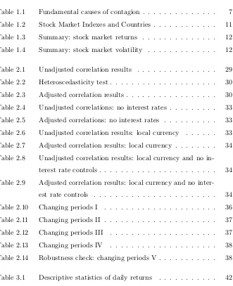
Table 1.1 Fundamental causes of contagion . . . 7

Table 1.2 Stock Market Indexes and Countries . . . 11

Table 1.3 Summary: stock market returns . . . 12

Table 1.4 Summary: stock market volatility . . . 12

Table 2.1 Unadjusted correlation results . . . 29

Table 2.2 Heteroscedasticity test . . . 30

Table 2.3 Adjusted correlation results . . . 30

Table 2.4 Unadjusted correlations: no interest rates . . . 33

Table 2.5 Adjusted correlations: no interest rates . . . 33

Table 2.6 Unadjusted correlation results: local currency . . . 33

Table 2.7 Adjusted correlation results: local currency . . . 34

Table 2.8 Unadjusted correlation results: local currency and no in-terest rate controls . . . 34

Table 2.9 Adjusted correlation results: local currency and no inter-est rate controls . . . 34

Table 2.10 Changing periods I . . . 36

Table 2.11 Changing periods II . . . 37

Table 2.12 Changing periods III . . . 37

Table 2.13 Changing periods IV . . . 38

Table 2.14 Robustness check: changing periods V . . . 38

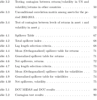
Table 3.1 Descriptive statistics of daily returns . . . 42

(11)

[image:11.439.71.399.46.384.2]

Table 3.2 Testing contagion between returns/volatility in US and

volatility/returns in other countries . . . 50

Table 3.3 Unconditional correlation matrix among assets for the pe-riod 2002-2013. . . 52

Table 3.4 Test of contagion between levels of returns in asseti and volatility in asset j. . . 52

Table 4.1 Spillover Table . . . 67

Table 4.2 Total spillover index . . . 68

Table 4.3 Lag length selection criteria . . . 68

Table 4.4 Mean (Orthogonalized) spillover table for returns . . . . 71

Table 4.5 Generalized spillover table for returns . . . 71

Table 4.6 Net spillovers, returns. . . 72

Table 4.7 Lag length selection criteria . . . 73

Table 4.8 Mean (Orthogonalized) spillover table for volatilities . . . 73

Table 4.9 Generalized spillover table for volatilities . . . 74

Table 4.10 Net spillovers, volatility. . . 75

Table 5.1 DCC MIDAS and DCC results . . . 89

(12)

[image:12.439.63.397.218.604.2]

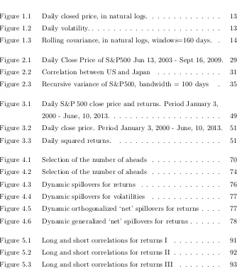
List of Figures

Figure 1.1 Daily closed price, in natural logs. . . 13

Figure 1.2 Daily volatility. . . 13

Figure 1.3 Rolling covariance, in natural logs, windows=160 days. . 14

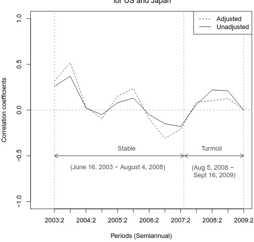
Figure 2.1 Daily Close Price of S&P500 Jun 13, 2003 - Sept 16, 2009. 29 Figure 2.2 Correlation between US and Japan . . . 31

Figure 2.3 Recursive variance of S&P500, bandwidth = 100 days . 35 Figure 3.1 Daily S&P 500 close price and returns. Period January 3, 2000 - June, 10, 2013. . . 49

Figure 3.2 Daily close price. Period January 3, 2000 - June, 10, 2013. 51 Figure 3.3 Daily squared returns. . . 51

Figure 4.1 Selection of the number of aheads . . . 70

Figure 4.2 Selection of the number of aheads . . . 74

Figure 4.3 Dynamic spillovers for returns . . . 76

Figure 4.4 Dynamic spillovers for volatilities . . . 77

Figure 4.5 Dynamic orthogonalized ‘net’ spillovers for returns . . . . 77

Figure 4.6 Dynamic generalized ‘net’ spillovers for returns . . . 78

Figure 5.1 Long and short correlations for returns I . . . 91

Figure 5.2 Long and short correlations for returns II . . . 92

Figure 5.3 Long and short correlations for returns III . . . 93

(13)

Chapter

1

International Financial Contagion: A review

“Blaming financial crises on

contagion has proved to be highly

contagious among economists and

politicians alike...”

(Moser, 2003, p.157)

This chapter is devoted to provide a review on the different definitions of what

contagion is, how it is measured, what causes contagion and mainly why it is

important to account for it when designing policies and undertaking the decision

making process.

Despite of the growing popularity of blaming “contagion” for international

financial crisis, contagion remains being an elusive concern. Without a clear

un-derstanding of financial contagion and the mechanisms through which it works, we

can neither assess the problem nor design appropriate policy measures to control

for it (Moser, 2003).

A growing literature has emerged in an attempt to study the implications of the

existence of financial contagion among countries. It is a clear fact that contagion

has important economic implications in terms of international policies carried out

by International Monetary Fund (IMF) jointly with the affected country or group

of countries, since bailouts funds lent by the IMF has a weakening effect over

the balance of payment of the countries when contagion is not evidenced as the

source of crisis for the borrower country. On the other hand, investors need to

(14)

Chapter 1

evaluate the potential benefits of international portfolio diversification as well as

the assessment of risks.

In the literature of financial contagion, there is yet little convergence of views

about whether cross-county propagation of shocks through fundamental should

be considered contagion. A number of authors call for discrimination between

‘pure contagion’ and shock propagation through fundamentals1_{, which suggest}

labeling ‘transmission’ (Bordo and Murshid, 2001), ‘spillovers’ (Masson, 1998),

interdependence (Forbes and Rigobon, 2001, 2002) or ‘fundamental-based

conta-gion’ (Kaminsky and Reinhart, 1998). According to Moser (2003) the main reason

for such discrimination is “that shocks propagation through fundamentals is the

result of an optimal response to external shocks”, which not constitutes a source

of ‘pure contagion’.

As a crisis in one country upsets the equilibrium in other countries, real and

financial variables adjust to a new equilibrium. Financial market responses only

reflect (anticipated) changes in fundamentals and speed up adjustment to the new

equilibrium, but they do not cause the change in equilibrium. In other words,

rather than causing the crisis, financial market responses bring the crisis forward,

this can be thought as an example of fundamental-based contagion which is not a

‘pure-contagion’ crisis (Moser, 2003).

Market imperfections are the key to rely on when trying to explain the

cross-country propagation of shocks when they are whether not related or explained by

the fundamentals. Moser (2003) distinguishes two groups to classify the

mecha-nisms of pure contagion:

1. Information Effects: information imperfections and costs of acquiring and

processing information make a correct assessment of fundamentals difficult

and a certain degree of ignorance rational. As a result, market participants

are uncertain about the true state of a country’s fundamentals. A crisis

elsewhere might lead them to reassess the fundamentals of other countries

and cause them to sell assets, to call in loans, or to stop lending to these

countries, even if their fundamentals remain objectively unchanged. The

literature offers a number of reasons why a crisis elsewhere could lead to a

reassessment of objectively unchanged fundamentals:

1_{Financial, real, and political links constitute the}_fundamentals_{of an economy.}

(15)

• Signal extraction failures2

• Wake-up call

• Expectations interaction

• Moral hazard plays

• Membership contagion

2. Domino Effects: In this group of explanations, a crisis in one country spreads

to others rather mechanically in domino fashion as a result of direct or

indi-rect financial connections. This story comes in three variations,

• Counterparty defaults

• Portfolio rebalancing due to liquidity constraints

• Portfolio rebalancing due to capital constraints

1.1 What is Financial Contagion?

The word contagion has been widely used in the economics literature to refer a

wide range of phenomena concerning financial economics, labor market, enterprise

and individual behavior and other spheres of the broad economy within

interre-lated activities are embed. From very ancient times, economists have used the

concept of contagion to refer situations such as: spread of bank runs and spread

of strikes across firms or industries (Mavor, 1891), the spread of increases secured

by labor unions to non-unions firms or sector (Ulman, 1955), the spread or

busi-ness fluctuations across economies (Mack and Zarnowitz, 1958), the diffusion of

technology and growth convergence across countries (Baumol, 1994; Findlay, 1978)

and the spread of the speculative trading across individuals (White, 1940), here

the common fact is the wordspread, denoting contagion as a synonym to either

spread or diffusion of something negative, namely contagion/spread of economic

problems. In modern times, the word contagion still has negative connotations

and is not an omen of good news.

In the recent literature, the concept is supposed to describe incidents in which

a (suitably defined) financial crisis in one country brings about a crisis in another.

In its broadest sense, therefore, financial contagion has to do with the propagation

(16)

Chapter 1

of adverse shocks that have the potential to trigger financial crises. The crux of

the matter is to identify potential propagation mechanisms and define those that

represent contagion (Moser, 2003). As a first step it is helpful to understand what

contagion does not mean and what does mean.

The first issue to be overcome to understand what contagion is has to do with

its modern definition, indeed there is a widespread disagreement around it.

The World Bank has three definitions of contagion: very restrictive, restrictive

andbroad definition, where the classification is based on the degree of restriction

which it has to do with the scope in terms of the events related to the timing,

state of the world and the difficulty/easiness to identify contagion.

Thevery restrictive definitionimplies increase in linkages after a crisis, so that

contagion occurs when cross-country correlations increase during “crisis times”

relative to correlations during “tranquil times”. Forbes and Rigobon (2002) define

contagion using the very restrictive definition, as a significant increase in

cross-market linkages after a (negative) shock to one country (or group of countries).

According to this definition, if two markets show a high degree of co-movement

during periods of stability, even if the markets continue to be highly correlated

after a (negative) shock to one market, this may not constitute contagion. It is

only contagion if cross-market co-movement increases significantly after the shock.

If the co-movement does not increase significantly, then any continued high-level of

market correlation suggests strong linkages between the two economies that exist in

all states of the world. Forbes and Rigobon (2002) use the term interdependence

to refer to this situation. Interdependence, as opposed to contagion, occurs if

cross-market co-movements is not significantly bigger after a (negative) shock to

one country or group of countries.

Currently this very restrictive definition is one of the most popular, because

it has two important advantages: first, it provides a straightforward framework

for testing whether contagion occurs or not by simply comparing linkages (such

as cross-market correlation coefficients) between two markets during a relatively

stable period with linkages after a shock or crisis and as a second benefit, it

pro-vides a straightforward method of distinguishing between alternative explanations

of how crises are transmitted across markets. Several works are based on this

definition: the seminal paper of King and Wadhwani (1990), Lee and Kim (1993)

(17)

and Reinhart and Calvo (1996), Forbes and Rigobon (2002), Naoui et al. (2010a),

Naoui et al. (2010b) and Wang and Nguyen Thi (2013), just to mention some of

them.

The second definition of the World Bank about contagion is the restrictive

definition: Contagion is the transmission of shocks to other countries or the

cross-country correlation, beyond any fundamental link among the countries and beyond

common shocks. This definition is usually referred as excess co-movement,

com-monly explained by herding behavior. there are three major works that can be

grouped into this category: Eichengreen et al. (1995), Eichengreen et al. (1996)

and Bekaert et al. (2005).

According to Dungey et al. (2003), there are still formidable difficulties in

reaching the appropriate set of fundamentals to use as control variables when

con-tagion analysis is performed under therestrictive definition, suggesting that such

models may not be effectively operational. Nevertheless, recent empirical research

proposes two alternative means: Dungey et al. (2003) propose the use of latent

factor models, which do not require the exact specification of the fundamental

relationships, while Pesaran and Pick (2004) suggest controlling for

fundamental-based market interdependencies using trade flow data and examining contagion as

transmissions above that.

The restrictive definition of contagion does not need any type of link among

countries, its nature only implies that contagion it is said to be explained by causes

beyond any fundamental links, namely, herd behavior, financial panics, or switches

of expectations across instantaneous equilibria (see Corsetti et al., 2001).

The third and last definition of contagion provided by The World Bank is

thebroad definition: Contagion is the cross-country transmission of shocks or the

general cross-country spillover effects. Furthermore, this definition also claims

that contagion can take place during both “good” times and “bad” times. Then,

contagion does not need to be related to crises. However, contagion has been

emphasized during crisis times.

Using the broad definition makes things harder since it does not provide the

researcher with a framework to work with, no triggering event is involved and,

a priori, no underlying relationships are supposed. Within this definition we can

(18)

Chapter 1

(2009) and Diebold and Yilmaz (2012). Corsetti et al. (2001) specify that

conta-gion occurs when country-specific shock becomes “reconta-gional” or “global”, this work

also belongs to thebroad definition of contagion.

Apart from the World Bank’s definitions there are also a number of ad hoc

definitions of contagion and that is why the use of the word ‘contagion’ to

de-scribe the international transmission of financial crises has become fraught with

controversy (Dungey and Tambakis, 2003).

This thesis uses the very restrictive definition of contagion, mainly for its

ad-vantages over the others and most importantly, because it provides an alternative

explanation for transmission of crisis, namely interdependence, then the natural

question on this context could beContagion or Interdependence?, try to answer

this question is the target of this thesis.

According to the definition of contagion chosen for this work, there should be

a shock as a cause of contagion and this is represented by a crisis. Thus, Corsetti

et al. (2001) claims that crises are characterized by what they call empirical

reg-ularities:

1. Sharp falls in stock markets tend to concentrate in periods of international

financial turmoil.

2. Volatility of stock prices increases during crisis periods.

3. Covariance between stock market returns increases during crisis periods.

4. Correlation between stock market returns is not necessarily larger during

crisis periods than during tranquil periods.

1.2 Causes of Contagion

According to Masson (1998); Dornbusch et al. (2000); Pristker (2000) and Forbes

and Rigobon (2001) the causes of contagion can be divided conceptually into two

categories: The first category emphasizes spillovers that result from the normal

in-terdependence among market economies. This inin-terdependence means that shocks,

whether of a global or local nature, can be transmitted across countries because

of their real and financial linkages. Reinhart and Calvo (1996) term this type of

crisis propagation “fundamentals-based contagion”. These forms of co-movements

(19)

[image:19.439.65.366.60.127.2]

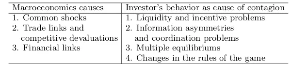
Table 1.1: Fundamental causes of contagion

Macroeconomics causes Investor’s behavior as cause of contagion 1. Common shocks 1. Liquidity and incentive problems 2. Trade links and 2. Information asymmetries

competitive devaluations and coordination problems 3. Financial links 3. Multiple equilibriums

4. Changes in the rules of the game

would not normally constitute contagion, in the sense of therestrictive and very

restrictivedefinitions.

The second category involves a financial crisis that is not linked to observed

changes in macroeconomics or other fundamentals but is solely the result of the

behavior of investors or other financial agents. Under this definition, contagion

arises when a co-movement occurs, even when there are no global shocks and

interdependence and fundamentals are not factors. A crisis in one country may,

for example, lead investors to withdraw their investments from many markets

without taking account of differences in economics fundamentals. This type of

contagion is often said to be caused by “irrational” phenomena, such a financial

panics, herd behavior, loss of confidence, and increased risk aversion. Some causes

of contagion are listed in Table 1.1.3_.

The degree of financial market integration determines how immune to contagion

countries are. The spread of a crisis depends on the degree of financial market

integration. The higher the degree of integration, the more extensive could be

the contagious effects of a common shock or a real shock to another country.

Conversely, countries that are not financially integrated, because of capital controls

or lack of access to international financing, are by definition immune to contagion

(Dornbusch et al., 2000). This is true in our definition of contagion, but it might

not be true under other definitions.

According to Forbes and Rigobon (2001), the theoretical literature of contagion

could be split into two groups: crisis-contingent and non-crisis-contingent

theo-ries. Crisis-contingent theories as its name suggests are those that explain why

transmission mechanisms change during a crisis and therefore why a shock leads to

increase the cross-market linkages. On the other hand, Non-crisis-contingent

the-ories assume that transmission mechanisms are the same during a crisis as during

(20)

Chapter 1

more stable periods, and therefore cross-market linkages do not change (increase)

after a shock. Theories belonging to the second group may be interpreted as pure

interdependence not as contagion.

Contagion may

be explained by

                                               Crisis-Contingent Theories            Multiple equilibria Endogenous liquidity Political economy Non-Crisis-Contingent Theories                    Trade Policy coordination Country reevalution

Random aggregate shocks

1.3 How contagion is testing?

Cross-market linkages can be measured by a number of different statistics, such

as the correlation in asset returns, the probability of speculative attack, or the

transmission of shocks or volatility (Forbes and Rigobon, 2001). This is the reason

why there are three types of general approaches to achieve the test for contagion: 1)

analysis of cross-market correlation coefficients, 2) probit models and 3) GARCH

frameworks.

Tests based on cross-market correlation coefficients are the most

straightfor-ward and have two advantages previously mentioned. These tests compare the

correlation between two markets during stable periods and turmoil periods and, if

cross-country correlation coefficients increase significantly after a shock (in the

tur-moil period), then there is evidence enough to believe that contagion occurs. The

first major paper that utilized this approach was King and Wadhwani (1990), they

test for an increase in cross-market correlations between the US, UK and Japan

and found that correlations increased significantly after the US crash. Then Lee

and Kim (1993) extended the analysis using up to 12 major markets and they find

evidence of contagion. Reinhart and Calvo (1996) use this approach to test for

contagion after 1994 Mexican Peso crisis and also find contagion from Mexico to

(21)

Asian and Latin American emerging markets. The most extensive analysis using

this framework was built by Goldfajn and Baig (1999) testing for contagion in

stock indexes, currency prices, interest rates, and sovereign spreads in emerging

markets during the 1997-1998 East Asian crisis, they reached the same conclusion:

contagion occurred.

The second approach to test for contagion is constituted by probability models

such as probit models. An extensive list of papers has included tests for contagion

using this approach, mainly because it is simple and uses simplifying assumptions

and exogenous events to identify a model and directly measure changes in the

prop-agation mechanism. Such list of papers covers Eichengreen et al. (1996), Goldfajn

and Baig (1999), Kaminsky and Reinhart (1998), and Forbes and Rigobon (2001).

One important conclusion from these papers is that trade is the most important

transmission mechanism through contagion spreads.

ARCH and GARCH framework constitute the third approach to test for

con-tagion; this implies the estimation of the variance-covariance matrix of the

trans-mission mechanism across countries which has been used to analyze the 1987 US

stock market crash. Hamao et al. (1990) and Chou et al. (1994) find evidence of

significant spillovers across markets but contagion did not occur. Another

exam-ple of this methodology is Longin and Solnik (1995), they consider seven OECD

countries from 1960 to 1990 and, by estimating a multivariate GARCH(1,1) as

input to test for a Constant Conditional Correlation (Bollerslev, 1990) rejected

the hypothesis of a Constant Conditional Correlation (CCC), nevertheless, such

rejection of the null hypothesis is not directed linked with the existence of

conta-gion. Other papers based on Dynamic Conditional Correlations (DCC) model of

Engle (2002), are aimed to investigate whether contagion occurs by looking into

the time-varying structure of the correlations are Naoui et al. (2010a) and Naoui

et al. (2010b).

1.4 Policy Implications

Evaluating whether contagion occurs is important for several reasons. First, a

crit-ical tenet of investment strategy is that most economic disturbances are country

specific, stock markets in different countries should display relatively low

(22)

Chapter 1

risk and increase expected returns. If contagion occurs after a negative shock,

however, market correlations would increase in bad states, which would

under-mine much of the rational for international diversification, because ignoring the

contagion can lead to poor portfolio diversification and an underestimation of risk.

Second, many models of investor behavior are based on the assumption that

in-vestors react differently after a large negative shock. Knowing if contagion occurs

is key to understand how individual behavior changes in good and bad states.

Third, many international institutions and policy makers worry that a negative

shock to one country can have a negative impact on financial flows to another

country—even if the fundamentals of the second economy are strong and there is

little real connection between the two countries. Even if this effect is temporary,

it could lead to a financial crisis in the second country—a crisis completely

un-warranted by the country’s fundamentals and policies. If this sort of contagion

exists, it could justify IMF intervention and the dedication of massive amounts of

money to stabilization funds. A short-term loan could prevent the second

econ-omy from experiencing a financial crisis. On the other hand, if the crisis is due

to interdependence instead of contagion, a bailout fund might reduce the initial

negative impact, but it does not avoid the crisis by itself. It only gives more time

to make necessary adjustments.

1.5 Data

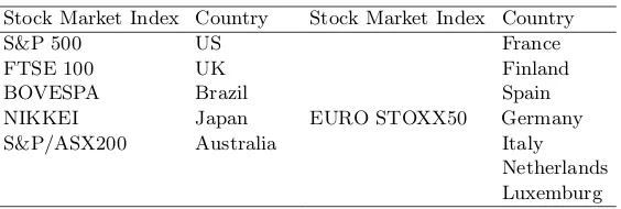
This section is devoted to introduce the dataset used throughout this thesis. Our

underlying data are daily nominal local-currency stock market indexes. We use

six aggregate stock market indexes covering twelve countries: eleven developed

stock markets (US, UK, Japan, Australia, France, Finland, Spain, Germany, Italy,

Netherlands and Luxembourg, all the European markets are grouped into one

unique index, Euro Stoxx50) and one emerging market (Brazil). Table 1.2 lists

the countries and stock indexes to be analyzed.

In Chapter 2 we also use the indexes from Table 1.2 in US dollars. Moreover

some interest rates are used as controls for global monetary shocks.

(23)

[image:23.439.79.361.60.155.2]

Table 1.2: Stock Market Indexes and Countries

Stock Market Index Country Stock Market Index Country

S&P 500 US France

FTSE 100 UK Finland

BOVESPA Brazil Spain

NIKKEI Japan EURO STOXX50 Germany

S&P/ASX200 Australia Italy

Netherlands Luxemburg

Daily stock prices are the inputs to calculate daily stock returns defined as

Rt= (lnPt−lnPt−1)×100 = ln

_P

t Pt−1

×100 (1.1)

Following Forbes and Rigobon (2002), stock market returns are calculated as

two days rolling-average, this allows us to control for the fact that markets in

different countries are not open during this same trading hours. For volatility we

assume that is fixed within periods (in this case, days) but variable across periods

and following Garman and Klass (1980) we use daily high, low, opening and closing

prices to estimate intraday volatility

˜

σ2t = 0.511(Ht−Lt)

2

−0.019[(Ct−Ot)(Ht+Lt−2Ot)−2(Ht−Ot)(Lt−Ot)]−0.383(Ct−Ot)2

(1.2)

whereHis the highest price in the day,Lis the lowest price,Ois the open day

price and C is the close price (all in natural logarithms), the estimated intraday

volatility will be the squared root of ˜σ2

t

Equation 1.2 is used in Chapter 4 as a proxy of the intraday volatility, however

in Chapter 5 a GARCH(1,1) process is estimated to account for the time varying

conditional volatility to be used in the Dynamic Conditional Correlation approach

undertaken in that chapter.

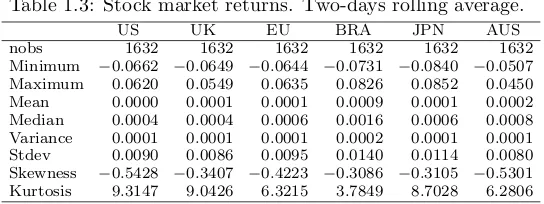
1.5.1 Descriptive statistics

Table 1.3 and Table 1.4 provide some insights about the sample for both returns

and volatility, respectively (in local currency). We use observations for daily

(24)

[image:24.439.84.356.52.154.2]

Chapter 1

Table 1.3: Stock market returns. Two-days rolling average.

US UK EU BRA JPN AUS

[image:24.439.93.349.205.298.2]

nobs 1632 1632 1632 1632 1632 1632 Minimum −0.0662 −0.0649 −0.0644 −0.0731 −0.0840 −0.0507 Maximum 0.0620 0.0549 0.0635 0.0826 0.0852 0.0450 Mean 0.0000 0.0001 0.0001 0.0009 0.0001 0.0002 Median 0.0004 0.0004 0.0006 0.0016 0.0006 0.0008 Variance 0.0001 0.0001 0.0001 0.0002 0.0001 0.0001 Stdev 0.0090 0.0086 0.0095 0.0140 0.0114 0.0080 Skewness −0.5428 −0.3407 −0.4223 −0.3086 −0.3105 −0.5301 Kurtosis 9.3147 9.0426 6.3215 3.7849 8.7028 6.2806

Table 1.4: Stock market volatility. Two-days rolling average.

US UK EU BRA JPN AUS

nobs 1632 1632 1632 1632 1632 1632 Minimum 0.0017 0.0021 0.0022 0.0034 0.0022 0.0012 Maximum 0.0690 0.0661 0.0759 0.0850 0.0653 0.0443 Mean 0.0090 0.0091 0.0098 0.0157 0.0095 0.0069 Median 0.0068 0.0070 0.0078 0.0137 0.0082 0.0053 Variance 0.0001 0.0000 0.0000 0.0001 0.0000 0.0000 Stdev 0.0074 0.0067 0.0068 0.0088 0.0058 0.0048 Skewness 3.4838 2.8296 3.0987 3.1279 3.2903 2.2544 Kurtosis 16.6433 11.6567 15.1026 15.4763 17.3575 7.7421

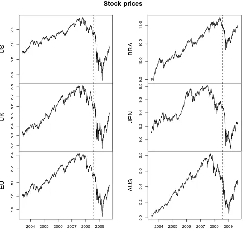
As an descriptive exercise, we plot daily stock prices, daily volatility and rolling

covariances (all in natural logs) to highlight theempirical regularities of a crisis.

According to Corsetti et al. (2001), when a crisis hits a stock market we would

expect sharp falls in prices, increases in volatility and also increases in covariances,

Figure 1.1, Figure 1.2 and Figure 1.3 behave accordingly to Corsetti et al. (2001)

regularities.

We plot the six markets’ volatilities and covariances in Figure 1.2 and in

Fig-ure 1.3, respectively, and immediately we can see that all volatilities and

covari-ances are higher during the crisis, with all markets displaying huge jumps. Since

August 2008, stock market volatility/covariances reflect the dynamics of the

sub-prime crisis quite well. The highest peak of S&P500 seen in Figure 1.2 was reached

on October 14, 2008.

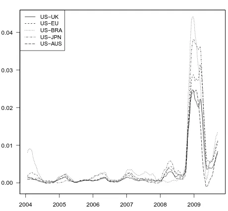
For the case of covariances, they are calculated using a moving windows of 160

days and only are plotted covariances corresponding to US with the other markets.

From the descriptives provided so far, we can see that the series capture quite

well the crisis and all of them behaves as described in theempirical regularities.

From Figure 1.1, Figure 1.2 and Figure 1.3 it seems that all stock markets reacted

(25)

6.6 6.8 7.0 7.2 US 8.2 8.3 8.4 8.5 8.6 8.7 8.8 UK

2004 2005 2006 2007 2008 2009

7.6 7.8 8.0 8.2 8.4 EU 9.5 10.0 10.5 11.0 BRA 9.0 9.2 9.4 9.6 9.8 JPN

2004 2005 2006 2007 2008 2009

[image:25.439.99.337.53.282.2]

8.0 8.2 8.4 8.6 8.8 A US Stock prices

Figure 1.1: Daily closed price, in natural logs.

0.00 0.02 0.04 0.06 US 0.00 0.02 0.04 0.06 UK

2004 2005 2006 2007 2008 2009

0.00 0.02 0.04 0.06 EU 0.02 0.04 0.06 0.08 BRA 0.00 0.02 0.04 0.06 JPN

2004 2005 2006 2007 2008 2009

0.00 0.01 0.02 0.03 0.04 A US

Two−days rolling average volatilities

[image:25.439.89.344.331.568.2]

(26)

Chapter 1

almost instantaneously to the shock hitting US which suggests that, somehow,

such shock spills over the other markets in the sample.

Moreover, Figure 1.3 suggests that the non-standardized unconditional

co-movements between US and the other countries were strengthened after the crisis,

they are relative low before US is hit by the crisis and after that event they rise

dramatically fast. If we divided the rolling covariances by the product of

corre-sponding rolling standard deviation, we would end up having the rolling

correla-tion which would suggest that, after the crisis, the linkages between US and other

countries increased giving rise to some suspects about the existence of contagion.

2004 2005 2006 2007 2008 2009 0.00

0.01 0.02 0.03 0.04

Covariances

[image:26.439.103.333.227.440.2]

US−UK US−EU US−BRA US−JPN US−AUS

Figure 1.3: Rolling covariance, in natural logs, windows=160 days.

1.6 Conclusions

Summarizing, this thesis is devoted to test the existence of contagion by means

of analyzing conditional co-movements, this analysis is not bounded by studying

only the first order co-movements, but it goes further and looks into higher order

co-movements to exploit some sort of asymmetries in the distribution of the series

when shifting from non-crisis to crisis periods. This study is focused on analyzing

the Subprime Crisis.

(27)

This introductory chapter shows that there is not a universally accepted

defini-tion of contagion, which is itself the first issue to be overcome. Through this entire

thesis, thevery restrictive definition provided by the World Bank is used as the

benchmark for contagion testing, because it explicitly provides a measure to assess

contagion, distinguishes two alternative channels through crises are spread all over

and recently it is becoming into the most popular tool to test for contagion.

For contagion to exist, according to the very restrictive definition, it is

nec-essary a crisis hitting one country or group of countries, additionally crises are

characterized by someempirical regularities which our data clearly exhibits.

Three general approaches have been used to test for contagion when crises

arrive, being the analysis of correlation the most extensively used. This thesis is

focused on testing the existence of contagion by means of analyzing conditional

movements, this analysis is not bounded by studying only the first order

co-movements, e.g., correlations, but also it looks into higher order co-movements to

exploit some sort of asymmetries in the distribution of the returns when shifting

from stable to turmoils periods

The existence of contagion implies a number of political implications. Within

the macroeconomics scope it has to do with portfolios rebalancing, positions of

the balance of payments for borrower countries, currency appreciations and all

its implications, just to mention few. In microeconomics terms, contagion can

influence in the rationality of agents and in extreme cases can lead to irrational

herding behavior provoking crisis and/or spreading crisis to other economies even

when their fundamentals are solid.

The reminding of this thesis consists of five more chapters. Chapter 2 is entitle

Contagion or Interdependence in the recent Global Financial Crisis? An

applica-tion to the stock markets using adjusted cross-market correlaapplica-tions. In this chapter

we use the very restrictive definition of contagion and we consider stock market

contagion as a significant increase in cross-market linkages after a shock to one

country or group of countries. Under this definition we study whether contagion

occurred from the U.S. Financial Crisis to the rest of the major stock markets in

the world by using the (adjusted) correlation coefficient approach developed by

Forbes and Rigobon (2002) which consists of testing whether cross-market

(28)

Chapter 1

The empirical strategy adopted in this chapter is using a vector autoregressive

(VAR) framework for estimating the dynamic relationship among markets and

afterwards performing the contagion test over the residual of the VAR previously

estimated. The VAR residuals constitute our returns net from fundamental effects

(Fry et al., 2010), therefore we use the VAR as a filter to distill any possible effect

of fundamentals over the series. After adjusting for heteroskedasticity bias in the

correlations as suggested by Forbes and Rigobon (2002), we failed in rejecting the

null hypothesis of interdependence between US and the i-th country embedded

in the sample. The empirical findings drawn from the analyzed sample strongly

suggest not contagion, only interdependence, this means that shocks, whether of

a global or local nature, can be transmitted across countries because of their real

and financial linkages (Masson, 1998; Dornbusch et al., 2000; Pristker, 2000; Forbes

and Rigobon, 2002).

In Chapter 3 we test for contagion adopting a different approach, the focus

in on co-skewness (Fry et al., 2010) which describes the feedback of shocks from

return to volatility and viceversa. The title of the chapter isWas the late 2008 US

Financial Crisis contagious? Testing using a higher order co-movement approach.

The starting point is the use of a generalized normal distribution that describes

the co-skewness parameters. This chapter is aimed by the fact that crisis heightens

the asymmetries in distribution of returns, so that looking into a higher order

co-movement statistics can provide a different and more complete information about

the transmission of shocks among countries. The contagion test based on the

co-skewness is somehow quite similar to that of based on correlations, there is

evidence of contagion if the co-skewness increases after a crisis. When taking into

account the asymmetries and adjusting for heteroskedasticity, the co-skewness test

suggests some evidence of contagion for feedback in higher order of co-movements.

Financial Spillover Across Countries: Measuring shock transmissions is the

ti-tle of the fourth chapter where we measure interdependence in returns as well as in

volatility among countries and summarizing into a spillover index. Spillover index

is based on the forecast error variance decomposition (fevd) from a VAR model

at h-step ahead forecast and we construct it using both the orthogonalized fevd

and the generalized fevd, both of them provide similar results, but the generalized

version is easier to handle, this is true since it does not depend on the

(29)

tions imposed by the Choleski decomposition, this fact makes it attractive when

economic theory is not available to identify variables relationship. This chapter is

accompanied by the development of an R package namedSpillovers to enable the

reproducibility of the methodology as well as performing co-skewness tests.

The fifth chapter is entitled A Component Model for Dynamic Conditional

Correlations: Disentangling Interdependence from Contagion. We propose using a

MIDAS-DCC with GARCH(1,1) (Colacito et al., 2011) component to asses both

contagion and interdependence. This methodology allows us to estimate both,

long-run and short-run correlations, we relate the former with interdependence as

this is driven by fundamentals and the latter is related with contagion episodes.

Spillovers: R package for estimating spillover indexes and performing

Co-Skewness test is the sixth chapter, which describes the package developed for

estimating the spillover indexes and performing co-skewness test. This package is

written using the R language (R Core Team, 2012) under the version 3.0.1. A user

manual is attached to this chapter on how to use theSpillovers package.

This thesis finishes with the seventh chapter which holds the general

(30)

Chapter 1

References

Baumol, W. J. (1994). Convergence of Productivity: Cross-National Studies and

Historical Evidence, chapter Multivariate Growth Patterns: Contagion and

com-mon forces as possible sources of convergence, pages 62–85. Oxford University

Press.

Bekaert, G., Harvey, C. R., and Ng, A. (2005). Market Integration and Contagion.

The Journal of Business, 78(1):39–70.

Bollerslev, T. (1990). Modelling the coherence in short-run nominal exchange

rates: A multivariate generalized arch model. The Review of Economics and

Statistics, 72(3):498–505.

Bordo, M. and Murshid, A. (2001). Are Financial Crises Becoming More

Con-tagious?: What is the Historical Evidence on Contagion? In Claessens, S.

and Forbes, K. J., editors,International Financial Contagion, pages 367–403.

Springer, 1 edition.

Chou, R. Y.-T., Ng, V., and Pi, L. K. (1994). Cointegration of International Stock

Market Indices. IMF Working Papers 94/94, International Monetary Fund.

Colacito, R., Engle, R. F., and Ghysels, E. (2011). A component model for dynamic

correlations. Journal of Econometrics, 164(1):45–59.

Corsetti, G., Pericoli, M., and Sbracia, M. (2001). Correlation Analysis of

Fi-nancial Contagion: What One Should Know Before Running a Test. Working

Papers 822, Economic Growth Center, Yale University.

Diebold, F. X. and Yilmaz, K. (2009). Measuring Financial Asset Return and

Volatility Spillovers, with Application to Global Equity Markets.The Economic

Journal, 119(534):158–171.

Diebold, F. X. and Yilmaz, K. (2012). Better to Give than to Receive:

Predic-tive Directional Measurement of Volatility Spillovers. International Journal of

Forecasting, 28(1):57–66.

Dornbusch, R., Park, Y. C., and Claessens, S. (2000). Contagion: Understanding

How It Spreads. World Bank Research Observer, 15(2):177–97.

(31)

Dungey, M., Fry, R., Martin, V., and Hermosillo, B. G. (2003). Unanticipated

Shocks and Systemic Influences: The Impact of Contagion in Global Equity

Markets in 1998. IMF Working Papers 03/84, International Monetary Fund.

Dungey, M. and Tambakis, D. (2003). International Financial Contagion: What

do we know? Working Papers 9, Australian National University.

Eichengreen, B., Rose, A. K., and Wyplosz, C. (1996). Contagious currency crises.

Scandinavian Journal of Economics, 98(4):463–484.

Eichengreen, B., Rose, A. K., Wyplosz, C., Dumas, B., and Weber, A. (1995).

Exchange Market Mayhem: The Antecedents and Aftermath of Speculative

Attacks. Economic Policy, 10(21):249–312.

Engle, R. (2002). Dynamic Conditional Correlation: A Simple Class of

Multivari-ate Generalized Autoregressive Conditional Heteroskedasticity Models. Journal

of Business & Economic Statistics, 20(3):339–350.

Findlay, R. (1978). Relative backwardness, direct foreign investment, and the

transfer of technology: A simple dynamic model. The Quarterly Journal of

Economics, 92(1):pp. 1–16.

Forbes, K. and Rigobon, R. (2001). Measuring contagion: Conceptual and

Empir-ical Issues. In Claessens, S. and Forbes, K. J., editors, International Financial

Contagion, page 480. Springer, 1 edition.

Forbes, K. and Rigobon, R. (2002). No Contagion, Only Interdependence:

Mea-suring Stock Market Comovements. The Journal of Finance, 57(5):2223–2261.

Fry, R., Martin, V. L., and Tang, C. (2010). A new class of tests of contagion with

applications. Journal of Business & Economic Statistics, 28(3):423–437.

Garman, M. B. and Klass, M. J. (1980). On the Estimation of Security Price

Volatilities from Historical Data. The Journal of Business, 53(1):67–78.

Goldfajn, I. and Baig, T. (1999). Financial market contagion in the Asian crisis.

(32)

Chapter 1

Hamao, Y., Masulis, R. W., and Ng, V. (1990). Correlations in Price Changes and

Volatility across International Stock Markets.The Review of Financial Studies,

3(2):281–307.

Kaminsky, G. L. and Reinhart, C. M. (1998). Financial Crises in Asia and Latin

America: Then and Now. The American Economic Review, 88(2):444–448.

King, M. A. and Wadhwani, S. (1990). Transmission of Volatility between Stock

Markets. The Review of Financial Studies, 3(1):5–33.

Lee, S. and Kim, K. J. (1993). Does the October 1987 crash strengthen the

comovements among national stock markets? Review of Financial Economics,

3:89–102.

Longin, F. and Solnik, B. (1995). Is the correlation in international equity returns

constant: 1960-1990? Journal of International Money and Finance, 14(1):3–26.

Mack, R. P. and Zarnowitz, V. (1958). Cause and consequence of changes in

retailers’ buying. The American Economic Review, 48(1):pp. 18–49.

Masson, P. R. (1998). Contagion-Monsoonal Effects, Spillovers, and Jumps

Be-tween Multiple Equilibria. IMF Working Papers 98/142, International Monetary

Fund.

Mavor, J. (1891). The scottish railway strike. The Economic Journal, 1(1):pp.

204–219.

Moser, T. (2003). What Is International Financial Contagion? International

Finance, 6(2):157–178.

Naoui, K., Khemiri, S., and Liouane, N. (2010a). Crises and Financial Contagion:

The Subprime Crisis. Journal of Business Studies Quaterly, 2(1):15–28.

Naoui, K., Liouane, N., and Brahim, S. (2010b). A Dynamic Conditional

Correla-tion Analysis of Financial Contagion: The Case of the Subprime Credit Crisis.

International Journal of Economics and Finance, 2(3):85–96.

Pesaran, M. and Pick, A. (2004). Econometric Issues in the Analysis of

Conta-gion. Cambridge Working Papers in Economics 0402, Faculty of Economics,

University of Cambridge.

(33)

Pristker, M. (2000). The Channels of Financial Contagion. The Contagion

Con-ference.

R Core Team (2012). R: A Language and Environment for Statistical Computing.

R Foundation for Statistical Computing, Vienna, Austria. ISBN 3-900051-07-0.

Reinhart, C. and Calvo, S. (1996). Capital Flows to Latin America: Is There

Evi-dence of Contagion Effects? MPRA Paper 7124, University Library of Munich,

Germany.

Ulman, L. (1955). Marshall and friedman on union strength. The Review of

Economics and Statistics, 37(4):pp. 384–401.

Wang, K.-M. and Nguyen Thi, T.-B. (2013). Did China avoid the Asian flu? The

contagion effect test with dynamic correlation coefficients.Quantitative Finance,

13(3):471–481.

White, Horace G., J. (1940). Foreign trading in american stock-exchange securities.

(34)

Chapter

2

Contagion or Interdependence in the recent Global

Financial Crisis? An application to the stock

markets using adjusted cross-market correlations

2.1 Introduction

During the last two decades, a growing literature has emerged in an attempt to

study the importance of the existence of financial contagion between countries. It

has been made clear that the existence of contagion has important economic

im-plications in terms of international policies taken and carried out by International

Monetary Fund (IMF) jointly with the affected country or group of countries.

Moreover, investors need to understand the nature of changes in correlations of

stock markets in order to evaluate the potential benefits of international portfolio

diversification as well as the assessment of risks.

We define contagion, following King and Wadhwani (1990) and Forbes and

Rigobon (2002), as a significant increase in cross-market linkages after a shock to

one country (or group of countries). According to this definition, contagion does

not occur if two markets show a high degree of co-movement during both stability

and crisis periods. The term interdependence is used instead if strong linkages

between the two economies exist in all states of the world. In the empirical analysis

we follow Forbes and Rigobon (2002) using the correlation approach corrected for

heteroskedasticity bias. Forbes and Rigobon (2002) call this approach adjusted

(35)

In this chapter we study empirically the recent 2008 - 2009 US Financial Crisis

using a straightforward approach based on cross-market correlation coefficients.

Our results indicate that there is no empirical evidence of contagion; instead, we

find evidence of interdependence in which the financial markets remain highly

correlated over time.

The empirical strategy adopted in this chapter is using a vector

autoregres-sive (VAR) framework for estimating the dynamic relationship among markets

and then performing the contagion test over the residual of the VAR previously

estimated. After adjusting for heteroskedasticity bias in the correlations as

sug-gested by Forbes and Rigobon (2002), we failed in rejecting the null hypothesis of

interdependence between US and any other country embedded in the sample. The

empirical findings drawn from the analyzed sample strongly suggest not contagion,

only interdependence, this means that shocks, whether of a global or local nature,

can be transmitted across countries because of their real and financial linkages

(Masson, 1998; Dornbusch et al., 2000; Pristker, 2000; Forbes and Rigobon, 2002).

The remainder of the chapter is arranged as follows. Section 2.2 discusses

the traditional technique of measuring stock market contagion showing that the

unadjusted correlation coefficient is biased, so adjusted correlation coefficient is

used to perform the hypothesis test. Section 2.3 presents the model and data

used to test for contagion while Section 2.4 discusses the results. Conclusions are

summarized in Section 2.5.

2.2 Unadjusted and adjusted Correlations

This section is set up to show the bias of the unadjusted correlation due to the

presence of heteroskedasticity.

Heteroskedasticity biases the cross-market correlation making the hypothesis

tests for contagion an inaccurate tool for identifying whether contagion exists

or not. For simplicity, the following discussion focuses on the two-market case.

Consider two stochastic variables, x and y both related through the following

equation:1

1_{Unadjusted Correlation is the term used by Forbes and Rigobon (2002) to refer to the}

(36)

Chapter 2

yt=α+βxt+t (2.1)

Considering the standard and classical assumptions for this Ordinary Least

Squares (OLS) regression we have:

E(t) = 0, (2.2)

E(2t) =c <∞, (2.3)

where c is a constant

E(xt, t) = 0 (2.4)

Assumptions (2.2), (2.3) and (2.4) ensure OLS estimation of (2.1) to be

consis-tent without omitted variables and with no endogeneity for both groups. Since we

are assuming two periods (precrisis and crisis) and no contagion, thereforeβh₌_βl_,

only these assumptions are required to make the proof and it is not required to

make further assumptions about the distribution of the residuals.

Now, consider two groups: one group with high variance (h) and the other one,

with the lower variance (l). Recall that in terms of our definition of contagion,

in the lower variance group corresponds to the period of relative market stability

and the high variance group is the period of turmoil, namely the period after

and including the crisis. By construction we know that σh

xx> σxxl , which when

combine with the standard definition ofβ:

βh₌ σ h xy σh

xx

= σ

l xy σl

xx

=βl_, _(2.5)

Given σh

xx> σlxx,it is clear that the covariance of each group is different and

it must be greater in the high volatility group than the lower one as noted in

Corsetti et al. (2001), this is because if theβ0_s_{are equal in the two groups and by}

construction we have statedσh

xx> σxxl , soσhxy> σlxy must be met. the empirical

regularities in Corsetti et al. (2001).

From (2.1) we can define the variance ofy as follows

σyy =β2σxx+σee (2.6)

(37)

and we can observe that since the variance of the residuals is assumed to remain

constant over the entire sample, this implies that the increase in the variance

of y across groups is less than proportional to the increase in the variance of x.

Therefore:

σxx σyy

h >

σxx σyy

l

. (2.7)

Finally, using the standard definition of the correlation coefficient we have:

ρh=ρl s

(1 +δ)

(1 +δ[ρl_]2₎, (2.8)

where ρh _{is the unadjusted correlation coefficient that depends on the relative}

increase in the variance, hence affected by heteroskedasticity, ρl _{is the adjusted}

correlation coefficient andδ is the relative increase in the variance ofx:

δ≡ σ

h xx σl

xx −

1. (2.9)

where (2.8)2 _{clearly shows that the estimated correlation coefficient is increasing}

inδ. Therefore, during periods of high volatility in marketx, the estimated

corre-lation (the unadjusted correcorre-lation) will be greater than the adjusted correcorre-lation,

even if the adjusted correlation coefficient remains constant over the entire period,

the unadjusted correlation coefficient will be biased upward and still being greater

than the adjusted correlation and this has direct implications to test for contagion

based on cross-market correlation coefficients.

This result implies that performing a test for contagion based on correlation

leads to wrongly accept the null hypothesis and conclude that contagion occurs

when this is false, providing a misleading conclusion.

Without adjusting for the bias, however, it is not possible to deduce if this

increase in the unadjusted correlation represents an increase in the adjusted

cor-relation or simply an increase in market volatility. According to our definition of

contagion, only an increase in the adjusted correlation coefficient would constitute

contagion.

2_{This same equation is also in Ronn et al. (2009), these authors called this equation as}

(38)

Chapter 2

The adjustment for this bias is a straightforward procedure under the

assump-tions discussed earlier and it only requires a simple manipulation of (2.8), solving

for the adjusted correlation coefficient (ρl_{) and renaming by} _ρ∗_{, yields}

ρ∗= ρ

h r

1 +δh1₋(ρh₎2i

(2.10)

Forbes and Rigobon (2002) prove that when a change greater than or equal to

a given absolute size in one of the variables is produced, the absolute magnitude

for the unadjusted correlation is increasing in the magnitude of that absolute

change. According to Forbes and Rigobon (2002), one potential problem with this

adjustment for heteroskedasticity is the assumption of no omitted variables and

not endogeneity between markets (written as (2.2) and (2.4)). In other words, the

proof of this bias and the adjustment is only valid if there are no exogenous global

shocks and no feedback from stock markety tox.

The same conclusion was reached by Ronn et al. (2009), they consider the

impact and implications of “large” changes in asset prices on the intra-market

correlations in the domestic and international markets, however Ronn et al. (2009)

use more restrictive assumptions about the distribution of the residuals. Actually,

(2.10) is also provided in Ronn et al. (2009).

2.3 Base Model and Data

Following Forbes and Rigobon (2002), we use a Vector Autoregressive (VAR)

framework to obtain a filtered version of the returns which are net of fundamentals

effects Fry et al. (2010). In order to deal with the non-synchronous trading times

we apply a 2-days rolling average to the filtered series, the specification of the

model is as follows

Xt=φ(L)Xt+ Φ(L)It+ηt (2.11)

Xt= n

xCt, x j t

o0

(2.12)

I=niCt, i j t

o0

(2.13)

(39)

Where xC

t is the stock market return in the crisis country; x

j

t is the stock

market return in another market j; Xt is a transposed vector of returns in the

same two stock markets;φ(L) and Φ(L) are vectors of lags;iC

t and i

j

t are

short-term interest rates for the crisis country and the country j, respectively; and ηt

is a vector of reduced-form disturbances used as the pre-filtered returns. For each

series of test, we first estimate the VAR model from (2.11). Once the VAR is

estimated, we proceed to estimate the variance-covariance matrices for each pair

of residuals during the full period, stable period and turmoil period. Afterwards,

from the information given by the variance-covariance matrices we calculate the

cross-market correlation coefficients for each set of countries and periods. Then,

we apply the Fisher Transformation to each correlation coefficients in order to

obtain a normal distribution of each of them.

Stock market returns are calculated as 2-days rolling-average based on each

country’s aggregate stock market index using US dollars as well as local currency,

but focus on US dollars returns since these were most frequently used in past work

on contagion, furthermore US dollars have the additional advantage of controlling

for inflation (under non-fixed exchange rate regimes). We utilize five lags3_for_φ₍_L₎

and Φ(L) in order to control for serial correlation and mainly for any within-week

variation in trading patterns. Interest rates have been included in order to control

for any aggregate shock and/or monetary policy coordination.4_{. An extensive set}

of sensitivity tests show that changing the model specification has no significant

impact on results.

We use six aggregate stock market indexes covering twelve countries. We

com-pare the correlation coefficients between US stock index and each stock index of

each single country. Countries and stock indexes are summarized in Table 1.2.

2.3.1 Hypothesis test

Using the specification in (2.11), we perform the test for stock market contagion.

The hypothesis test consists of determining whether there is a significant increase

3 _{A VAR Lag Order Selection Criteria was applied to select the best length of lag for the}

VAR estimation, the result of this was 5 lags as the best order.

4_{As Forbes and Rigobon (2002) remarked, interest rates are an imperfect measure of aggregate}

(40)

Chapter 2

in cross-market correlation coefficients after a shock, according to our definition

of contagion we establish the following hypothesis:

H0:ρ∗≥ρh

H1:ρ∗< ρh.

Whereρ∗_{is the correlation during the full period and}_ρh_{is the correlation}

dur-ing the turmoil period. Moreover, H0 represents the interdependence hypothesis

andH1 is contagion. The t-statistic has the following form:

t-stat =

1 2ln

h_{1+ ˆ}_ρh 1−ρˆh i

−1 2ln

h_{1+ ˆ}_ρ∗

1−ρˆ∗ i

r

1

nh−3

+_n_l1₋₃

. (2.14)

Test statistics and results are reported in the next section.

2.4 Results

Using the US Financial Crisis as the event to drive contagion, we define our period

of turmoil from August 5th, 2008 to September 16th, 2009. We define the period

of relative stability as lasting from June 16th, 2003 to the start of the period of

turmoil. The choice of the dates was made as a result from an analysis of the

S&P500 behavior which is depicted in Figure 2.1 and this selection of dates also

coincide with the World Bank’s Crisis Timeline; but the extensive robustness tests

performed below will show that period definition does not affect the central results.

The VAR models estimated in order to obtain the cross-market correlation

coefficients are stable and none of the variables considered for these estimations

have unit root, hence the hypothesis test performed for testing whether contagion

occurred or not is valid and it is only affected by the presence of heteroskedasticity5

and assuming that (2.2), (2.3) and (2.4) hold.

The estimated unadjusted correlation coefficients for stable, turmoil, and full

period are shown in Table 2.1. Since Fisher transformation ensures normality, we

use the normal critical value at 95%. The critical value for the t-test at the 5%

level is 1.65, so any test statistic greater than this critical value indicates contagion

(C), while any statistic less than or equal to this value indicates no contagion (N).

5_{No omitted variables is an assumption considered in this test.}

(41)

800 1000 1200 1400 1600

S&P500, 2003−2009

Close Pr

ice

2003−06−16 2004−10−06 2006−01−27 2007−05−22 2008−09−11

Stable (Pre−crisis) Turmoil

(Crisis)

Full period: Jun/13/2003 − Sept/16/2009

[image:41.439.50.379.84.282.2]

Stable (Pre−crisis) period: Jun/13/2003 − Aug/04/2008 Turmoil (Crisis) period: Aug/05/2008 − Sept/16/2009

Figure 2.1: Daily Close Price of S&P500 Jun 13, 2003 - Sept 16, 2009.

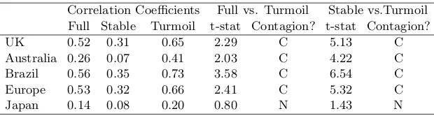
We can observe that the average unadjusted correlation coefficient increased

from 0.23 in the stable period to 0.53 in the turmoil period, it even has an

in-crease from 0.40 in the full period to the 0.53 in the high volatility period. But, as

previously discussed, these tests for contagion might be inaccurate due to the bias

resulting from heteroskedasticity. The estimated increases in the unadjusted

cor-relation could reflect either an increase in cross-market linkages and/or increased

market volatility (Forbes and Rigobon, 2002). Before making the adjustment for

Table 2.1: Unadjusted correlations

Correlation Coefficients Full vs. Turmoil Stable vs.Turmoil Full Stable Turmoil t-stat Contagion? t-stat Contagion?

UK 0.52 0.31 0.65 2.29 C 5.13 C

Australia 0.26 0.07 0.41 2.03 C 4.22 C

Brazil 0.56 0.35 0.73 3.58 C 6.54 C

Europe 0.53 0.32 0.66 2.41 C 5.32 C

Japan 0.14 0.08 0.20 0.80 N 1.43 N

[image:41.439.64.374.475.558.2]

Essays on financial contagion

ESSAYS ON FINANCIAL CONTAGION

Jilber Andrés Urbina Calero

Dipòsit Legal: T. 181-2014

ESSAYS ON FINANCIAL CONTAGION

by

Jilber Andr´es Urbina Calero

UNIVERSITAT ROVIRA I VIRGILI

Faculty of Economics and Business

Department of Economics

DOCTORAL THESIS

Jilber Andr´es Urbina Calero

ESSAYS ON FINANCIAL CONTAGION

DOCTORAL THESIS

Submitted to the Department of Economics

in partial fulfillment of the requirements for the degrees of

Doctor of Philosophy

at the

Universitat Rovira i Virgili

Supervised by:

Dr. Nektarios Aslanidis

Dr. Oscar Mart´ınez

Reus

Acknowledgment

Contents

List of Tables

List of Figures

Chapter

1

International Financial Contagion: A review

1.1

What is Financial Contagion?

1.2

Causes of Contagion

1.3

How contagion is testing?

1.4

Policy Implications

1.5

Data

1.6

Conclusions

References

Chapter

2

Contagion or Interdependence in the recent Global

Financial Crisis? An application to the stock

markets using adjusted cross-market correlations

2.1

Introduction

2.2

Unadjusted and adjusted Correlations

2.3

Base Model and Data

2.4

Results