Analysis and design of real-time control systems with varying control timing constraints

Texto completo

(1)UNIVERSITAT POLITÈCNICA DE CATALUNYA Deptartament d’Enginyeria de Sistemes, Automàtica i Informàtica Industrial. Programa de doctorat: Enginyeria en Informàtica Industrial / Tecnologies Avançades de la Producció. Tesi doctoral. Analysis and Design of Real-Time Control Systems with Varying Control Timing Constraints Pau Martí Colom. Directors:. Dr. Josep M. Fuertes. Dr. Gerhard Fohler. Dept. d’Enginyeria de Sistemes, Automàtica i Informàtica Industrial Universitat Politècnica de Catalunya. Dept. of Computer Engineering Mälardalen University. Barcelona, juny de 2002.

(2)

(3) A la Belén.

(4)

(5) Agraïments No hauria estat possible realitzar aquesta tesi sense l’ajuda de moltes persones. A totes elles, moltíssimes gràcies! It would not have been possible to produce this thesis without the help of many people. To all of them, thanks a lot!. Primerament, vull donar les gràcies als dos directors, el Dr. Josep Mª Fuertes (del departament d’Enginyeria de Sistemes, Automàtica i Informàtica Industrial de la Universitat Politècnica de Catalunya) i el Dr. Gerhard Fohler (del Computer Engineering Department de la Mälardalen University, Sweden) per haver-me dirigit, tant a nivell científic com humà, el procés d’aprenentatge en la realització d’aquesta tesi. Moltes gràcies! En el camí que m’ha conduït fins aquí, són moltes les persones que m’he anat trobant. Cada una d’elles forma part d’aquesta tesi. En un ordre cronològic i sense pretendre ser exhaustiu: Gràcies Pep per confiar en mi i ajudar-me en aquest món del control, tan complex per a mi. Thanks Gerhard for making me feel so welcome and guiding me throughout my real-time systems research. Thanks a lot to everybody living up there, in Sweden, for making me feel at home. Thanks Sashi, thanks Radu and Camilla, and thanks Thomas and Damir. Els meus agraïments també estan dirigits al Dr. Ricard Villà: moltes gràcies per la teva agudesa i les teves valuoses i imprescindibles aportacions. I also want to spend a few words to thank Prof. Krithi Ramamritham. Thanks Krithi for all the stimulating discussions we had, and for agreeing to collaborate in the work done in this thesis. Thanks for your contributions. Thanks also to Anton Cervin. Without your help, this thesis wouldn’t be like it is. Gràcies també a totes les persones que ara no cito i sense les quals aquest treball no hauria estat una realitat. Especialment, gràcies a la gent del departament, que d’una manera o altra, sempre m’han ajudat. No m’oblido dels meus amics i amigues: gràcies per estar sempre al meu costat! Pels ànims i suport que sempre m’heu donat, gràcies família!. I finalment, gràcies a tu Belén, per tot!.

(6)

(7) El treball realitzat en aquesta tesi ha estat parcialment financiat per: •. Projecte Metodologias de Diseño y Evaluación de Prestaciones en los Sistemas Distribuidos de Control. Ref. CICYT TAP98-0585-C03-01. •. Projecte Arquitecturas de Control Distribuido. Análisis y Diseño de Estructuras con Soporte de Tecnologias Internet-Intranet. Ref. CICYT DPI2000-1760-C03-01. •. Network of Excellence. Advanced Real Time Systems (ARTIST). Information Society Technologies. Ref. IST-2001-34820. •. Beques per a la recerca a fora de Catalunya (Generalitat de Catalunya), convocatòries 2000 i 2001. •. Pla de mobilitat externa del professorat UPC (Universitat Politècnica de Catalunya), convocatòries 1999, 2000, 2001 i 2002.

(8)

(9) Aquesta tesi s’ha realitzat durant la meva contractació com a professor associat en el Departament d’Enginyeria de Sistemes, Automàtica i Informàtica Industrial de la Universitat Politècnica de Catalunya. Tanmateix, vull destacar la importància que en la realització d’aquesta tesi han tingut les meves estades de recerca (Juliol de 1999, Juny de 2000, Gener i Juliol de 2001, Gener de 2002) al Real-Time Systems Lab (SDL) del Mälardalen Real-Time Research Centre (MRTC), Department of Computer Engineering, Mälardalen University, Sweden..

(10)

(11) Analysis and Design of Real-Time Control Systems with Varying Control Timing Constraints Summary The analysis and design of real-time control systems is a complex task, requiring the integration and good understanding of both control and real-time systems theory. Traditionally, such systems are designed by differentiating two separate stages: first, control design and then its computer implementation, leading to sub-optimal solutions in terms of both system schedulability and controlled systems performance. Traditional discrete-time control models and methods consider implementation constraints only to a very small extent. This is due to the fact that in the control design stage, controllers are assumed to execute in dedicated processors and processors are assumed to be fast and deterministic enough not to worry about the timing that the controlling activities may have on the implementation. However, when resources (e.g., processors) are limited, timing variations in the execution of control algorithms occur. Specifically, a control algorithm in traditional real-time scheduling is implemented as a periodic task characterized by standard timing constraints such as period and deadline. In real-time scheduling, timing variations in task instance executions (i.e., jitters) are allowed as far as the schedulability constraints are preserved. Consequently, the resulting jitters for control task instances do not comply with the strict timing demanded by discrete-time control theory. This has two pervasive effects: the presence of jitters for control tasks degrades the controlled system performance, even causing instability. On the other hand, minimizing the likelihood of jitters for control tasks by over-constraining the control task specification reduces the schedulability of the entire task set. It is worth mentioning that control theory offers no advice on how to include, into the design of controllers, the effects that implementation constraints have in the timing of the control activities (e.g., scheduling inherent jitters). Also, real-time theory lacks task models and timing constraints that can be used to guarantee a periodic task execution free of jitters without over-constraining system schedulability. In this thesis we present a flexible integrated scheduling and control analysis and design framework for real-time control systems that solves the problems outlined above: poor system schedulability and controlled systems performance degradation. We show that by merging the activities of the control and real-time communities, that is, by integrating control design with computer implementation, both system schedulability and controlled systems performance are improved. We present a new approach to discrete-time controller design that takes implementation constraints into account and relaxes the equidistant sampling and actuation assumptions of traditionally designed discrete-time controllers. Instead of specifying a single value for the sampling period and a single value for the time delay at the design stage, we specify a set of.

(12) values for both the sampling period and for the time delay. This new approach for the controller design relies on the idea of adjusting controller parameters at run time according to the specific implementation timing behaviour, i.e., scheduling inherent jitters. The resulting closed-loop systems are based on irregularly sampled discrete-time system models with varying time delays. We have used state space formulation to present a complete stability and response analysis for such models. We also show how to derive more flexible timing constraints for control tasks by exploiting the timing properties imposed by this new approach to discrete-time controller design. Realtime scheduling standard timing constraints for periodic tasks are constant for all task instances. That is, a single value of a constraint (e.g., period or deadline) holds for all task instances. Our flexible timing constraints for control tasks do not set specific values. Rather, they provide ranges and combinations to choose from (at each control task instance execution), taking into account, for example, schedulability of other tasks. That is, these more flexible timing constraints for control tasks allow us to obtain feasible schedules and stable control systems from task sets (including control and non-control tasks) that are not feasible using traditional real-time scheduling and discrete-time control design methods. In addition, by associating control performance information with these new timing constraints for control tasks, we show how scheduling decisions, going beyond meeting timing constraints, can be taken to improve the performance of the controlled systems when they are affected by perturbations..

(13) Anàlisi i Disseny de Sistemes de Control de Temps Real amb Restriccions Temporals Variables de Control Resum L’anàlisi i el disseny dels sistemes de control de temps real és una tasca complexa, que requereix la integració de dues disciplines, la dels sistemes de control i la dels sistemes de temps real. Tradicionalment però, els sistemes de control de temps real s’han dissenyat diferenciant, de forma independent, dues fases, primerament el disseny del controlador, i després, la seva implementació en un computador. Això ha desembocat en solucions no òptimes tant en termes de planificabilitat del sistema i com en el rendiment dels sistemes controlats. Normalment, els mètodes i models de la teoria de control de temps discret no consideren durant la fase de disseny dels controladors les limitacions que es puguin derivar de la implementació. En la fase de disseny s’assumeix que els algorismes de control s’executaran en processadors dedicats i que els processadors seran prou ràpids i determinístics per no haver-se de preocupar del comportament temporal que aquests algorismes de control tindran en temps d’execució. Tot i així, quan els recursos - per exemple, processadors - són limitats, apareixen variacions temporals en l’execució dels algorismes de control. En concret, en els sistemes de planificació de tasques de temps real, un algorisme de control s’implementa en una tasca periòdica caracterizada per restriccions temporals estàndards com períodes i terminis. És sabut que, en la planificació de tasques de temps real, les variacions temporals en l’execució d’instàncies de tasques és permesa sempre i quan les restriccions de planificabilitat estiguin garantides. Aquesta variabilitat per tasques de control viola l’estricte comporament temporal que la teoria de control de temps discret pressuposa en l’execució dels algorismes de control. Això té dos efectes negatius: la variabilitat temporal en l’execució de les tasques de control degrada el rendiment del sistema controlat, fins i tot causant inestabilitat. A més, si es minimitza la probabilitat d’aparició d’aquesta variabilitat en l’execució de les tasques de control a través d’especificacións més limitants, la planificabilitat del conjunt de tasques del sistema disminueix. Cal tenir en compte que la teoria de control no dóna directrius de com incloure, en la fase de disseny dels controladors, aquesta variabilitat en l’execució de tasques que es deriva de les limitacions d’implementació. A més, la teoria de sistemes de temps real no proporciona ni models de tasques ni restriccions temporals que puguin ser usats per garantir l’execució periòdica, i sense variabilitats temporals, de tasques sense sobrelimitar la planificabilitat dels sistema. En aquesta tesi es presenta un entorn integrat i flexible de planificació i de control per a l’anàlisi i el disseny de sistemes de control de temps real que dóna solucions als problemes.

(14) esmentats anteriorment (baixa planificabilitat en el sistema i degradació del rendiment dels sistemes controlats). Mostrem que, fusionant les activitats de la comunitat de temps real amb les de la comunitat de control, això és, integrant la fase de disseny de controladors amb la fase d’implementació en un computador, es millora tant la planificabilitat del sistema com el rendiment dels sistemes controlats. També es presenta una nova aproximació al disseny de controladors de temps discret que té en compte les limitacions derivables de la implementació i relaxa les tradicionals assumpcions dels controladors de temps discret (mostreig i actuació equidistants). En lloc d’especificar, en la fase de disseny, únics valors pel període de mostreig i pel retard temporal, especifiquem un conjunt de valors tant per l’un com per l’altre. Aquesta nova aproximació al disseny de controladors es basa en la idea d’ajustar, en temps d’execució, els paràmetres del controlador d’acord amb el comportament temporal específic de la implementació (per exemple, d’acord amb la variabilitat en l’execució de les tasques deguda a la planificació). Els llaços de control resultants esdevenent sistemes variants en el temps, amb mostreig irregular i retards temporals variables. Per a aquests sistemes, i utilitzant formulació en l’espai d’estat, presentem una anàlisi completa d’estabilitat, així com l’anàlisi de la resposta. També mostrem com, a partir de les propietats temporals d’aquesta nova aproximació al disseny de controladors, podem obtenir restriccions temporals més flexibles per a les tasques de control. Les restriccions temporals estàndards, per a les tasques periòdiques en els sistemes de temps real, són constants per a totes les instàncies d’una tasca. Això és, només un sol valor per a una restricció és aplicable a totes les instàncies. Les noves restriccions temporals que presentem per a tasques de control no forcen a aplicar un valor específic, sinó que permeten aplicar valors diferents a cada instància d’una tasca, tenint en compte, per exemple, la planificabilitat d’altres tasques. Aquestes restriccions temporals flexibles per a tasques de control ens permeten obtenir planificacions viables i sistemes de control estables a partir de conjunts de tasques (incloent tasques de control i d’altres) que no eren planificables en usar mètodes estàndards tant de planificació de temps real com de disseny de controladors. A més, associant informació de rendiment de control a aquestes noves restriccions temporals per a tasques de control, mostrem com podem prendre decisions de planificació que, anant més enllà de complir amb les restriccions temporals, milloren el rendiment dels sistemes controlats quan aquests sofreixen perturbacions..

(15) Contents 1. 2. 3. 4. Introduction. 1. 1.1 1.2 1.3 1.4. 2 3 5 6. Motivation Objectives System model Thesis structure. Background and state of the art. 9. 2.1 Real-time systems 2.1.1 Task constraints 2.1.2 Real-time scheduling 2.2 Control systems 2.2.1 Analysis and design of control systems 2.2.2 Computer control 2.3 State of the art 2.3.1 Feedback control real-time scheduling 2.3.2 Control approaches 2.3.3 Scheduling approaches 2.3.4 Control and scheduling integration 2.4 Summary. 9 10 11 17 19 24 32 32 33 34 34 36. Control impact on schedulability. 37. 3.1 Discrete-time control theory timing analysis 3.1.1 Closed-loop timing assumptions 3.1.2 From theoretical timing to applied timing 3.2 Control systems schedulability 3.2.1 Mapping control timing requirements to real-time task timing constraints 3.2.2 Real-time implementation of closed-loops 3.2.3 Limits of control task scheduling 3.3 Summary. 37 38 42 45 44 46 48 51. Schedulability impact on control. 53. 4.1 Real-time scheduling timing analysis 4.1.1 Jitters characterization 4.1.2 Effects of scheduling inherent jitters on control tasks 4.1.3 Sampling jitter and sampling-actuation jitter properties 4.2 Jitter impact on control 4.2.1 Illustrative examples 4.2.2 Impact explanation 4.3 Summary. 53 53 56 60 62 62 67 69.

(16) 5. 6. 7. 8. Integrated scheduling and control co-design. 71. 5.1 5.2 5.3 5.4 5.5. 71 73 74 74 77. Motivation Flexible control design Flexible timing constraints for control tasks Applications Summary. Adapting control algorithms to implementation constraints. 79. 6.1 Control algorithms design adjustment 6.1.1 Problem definition 6.1.2 Closed-loop implementation effects on the controller timing parameters 6.1.3 Summary of the variation in the controller timing parameters 6.1.4 Completeness of the compensation approach 6.2 Controller design problem formulation 6.2.1 Irregularly sampled discrete-time system model 6.2.2 Discrete-time system model with varying time delays 6.2.3 Irregularly sampled discrete-time system model with varying time delays 6.2.4 Sequences of feasible sampling intervals and sampling-actuation delays 6.3 Summary. 79 79 81 87 89 89 90 93 95 96 97. Flexible discrete-time controller design. 99. 7.1 Compensation approach controller design method 7.1.1 Closed-loop system response analysis 7.1.2 Stability analysis 7.1.3 Summary 7.1.4 Example 7.2 Practical implementation considerations 7.2.1 Temporal information required for the parameters adjustment 7.2.2 Controller parameters adjustment code implementation details 7.2.3 Computational overhead 7.2.4 Memory requirements 7.3 Summary. 99 100 101 103 104 107 107 110 114 115 116. Compensation approach in standard real-time scheduling policies. 117. 8.1 Compensation approach as a control-based solution for dealing with jitters 8.1.1 Requirements of the compensation approach in real-time scheduling 8.1.2 Application of the compensation approach for scheduled control tasks 8.1.3 Examples 8.2 Compensation approach control performance evaluation 8.2.1 Performance criterion selection 8.2.2 Evaluation study 8.3 Summary. 117 118 120 123 130 130 134 139.

(17) 9. Flexible control task scheduling. 141. 9.1 Control task scheduling with flexible timing constraints 9.1.1 Fixed timing constraints for control tasks 9.1.2 Flexible timing constraints for control tasks 9.1.3 Example 9.2 Quality-of-control (QoC) scheduling 9.2.1 Quality-of-control criterion definition 9.2.2 Influence of different instance separation sequences on the QoC 9.2.3 Formulation of the QoC scheduling problem 9.2.4 Solution for the QoC scheduling problem 9.3 Summary. 141 142 143 145 147 148 151 153 156 163. 10 Conclusions 10.1 Contributions 10.2 Future work References Appendices A, B and C. 165 168 169 171.

(18)

(19) List of Figures Figure Pg. 1.1 System model scheme 5 1.2 Node level scheme 5 2.1 Task structure 10 2.2 Sequence of instances for a periodic task 10 2.3 Task instance description 11 2.4 Offline schedule 14 2.5 Run time execution of the offline schedule of Figure 2.4 14 2.6 Example of schedule produced by EDF 15 2.7 Example of schedule produced by RM 16 2.8 Process to be controlled 17 2.9 Open-loop (also called feedforward) control system 17 2.10 Closed-loop (also called feedback) control system 18 2.11 Subsystems in a closed-loop control system 18 2.12 (a) Stable, (b) marginally stable or (c) unstable linear time-invariant control 21 system 2.13 Linear time-invariant control system stability according to the closed-loop 21 poles location in the (a) s-plane and (b) z-plane 2.14 Unit step response of a standard second order system. 22 2.15 Right - Closed-loop system. Left - System error 23 2.16 Diagram of a computer-controlled system 24 2.17 PID discretization 27 2.18 PID controller implementation in a control task 27 2.19 DC servo system response showing the reference signal tracking 27 2.20 Inverted pendulum 28 2.21 State feedback controller implementation in a control task 29 2.22 Inverted pendulum system response 29 2.23 Inverted pendulum system response for different sampling periods 31 2.24 Inverted pendulum system response for different time delays (complete view - 32 left- and detailed view –right.) 3.1 Timing assumptions of regularly sampled discrete-time system models 39 3.2 Timing assumptions of regularly sampled discrete-time system models with 40 constant time delays 3.3 Timing assumptions of regularly sampled discrete-time system models with 40 actuation at the next sampling instant 3.4 Input-output synchronization depending on the time delay: (left) τ = 0, 41 (middle) 0 < τ < h and (right) τ = h 3.5 Local (left) vs. distributed (right) closed-loop system 43 3.6 Closed-loop implemented using a single periodic task 47 3.7 Closed-loop implemented using multiple periodic tasks 47 3.8 Feasible offline schedule 48.

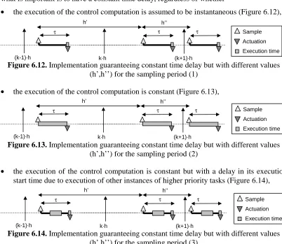
(20) 3.9 3.10 3.11 3.12 4.1 4.2 4.3 4.4 4.5 4.6 4.7 4.8 4.9 4.10 4.11 4.12 4.13 6.1 6.2 6.3 6.4 6.5 6.6 6.7 6.8 6.9 6.10 6.11 6.12 6.13 6.14 6.15 6.16 6.17. Possible orderings for task1 Possible orderings for task2 Feasible schedule of two control tasks with strict harmonic period relation Feasible schedule of two control tasks with soft harmonic period relation Jitters in task instances Partial schedule corresponding to RM Sampling jitter: partial schedule Sampling-actuation jitter: partial schedule Sampling jitter and sampling-actuation jitter: partial schedule Maximum and minimum sampling intervals Maximum and minimum sampling-actuation delays DC servo response (left - expected response) with jitter degradation (right) RM partial schedule for the task set over the task periods LCM (26ms) RM (top) and EDF (bottom) partial schedule for the task set over the task periods LCM EDF (left) and RM (right) sampling jitter degradation EDF (left) and RM (right) sampling-actuation jitter degradation EDF (left) and RM (right) sampling jitter and sampling-actuation jitter effects on the inverted pendulum response Implementation guaranteeing equidistant sampling Implementation guaranteeing equidistant sampling and constant time delay (1) Implementation guaranteeing equidistant sampling and constant time delay (2) Implementation guaranteeing equidistant sampling and constant time delay (3) Implementation guaranteeing equidistant sampling and constant time delay (4) Implementation guaranteeing equidistant sampling and constant time delay (5) Implementation guaranteeing equidistant sampling but with different values (τ’,τ’’) for the time delay (1) Implementation guaranteeing equidistant sampling but with different values (τ’,τ’’) for the time delay (2) Implementation guaranteeing equidistant sampling but with different values (τ’,τ’’) for the time delay (3) Implementation guaranteeing equidistant sampling but with different values (τ’,τ’’) for the time delay (4) Implementation that does not guarantee equidistant sampling Implementation guaranteeing constant time delay but with different values (h’,h’’) for the sampling period (1) Implementation guaranteeing constant time delay but with different values (h’,h’’) for the sampling period (2) Implementation guaranteeing constant time delay but with different values (h’,h’’) for the sampling period (3) Implementation guaranteeing constant time delay but with different values (h’,h’’) for the sampling period (4) Implementation guaranteeing constant time delay but with different values (h’,h’’) for the sampling period (5) Implementation with different values for the sampling period (h’, h’’) and. 49 49 50 51 54 55 58 58 59 60 61 62 63 64 64 66 66 82 82 82 82 83 83 83 84 84 84 85 85 85 85 86 86 86.

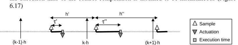
(21) time delay (τ’, τ’’) (1) 6.18 Implementation with different values for the sampling period (h’, h’’) and time delay (τ’, τ’’) (2) 6.19 Implementation with different values for the sampling period (h’, h’’) and time delay (τ’, τ’’) (3) 6.20 Implementation with different values for the sampling period (h’, h’’) and time delay (τ’, τ’’) (4) 6.21 Control implementation problem formulation scheme 7.1 Inverted pendulum responses if the controller is characterized each time for one of all possible combinations of feasible sampling intervals and feasible sampling-actuation delays. 7.2 Two of all the possible responses of Figure 7.1 (dotted) and the compensated (solid curve) 7.3 Feasible sampling interval measurement 7.4 Feasible sampling-actuation delay measurement 7.5 Left - generic controller code. Right - compensation approach controller code 7.6 Top - Classic PID code. Bottom - Compensated PID code 7.7 Top - Classic state feedback controller code designed using pole placement. Bottom – Compensated state feedback controller code designed using pole placement 7.8 Compensated State Feedback Controller code designed through pole placement with access to the controller parameters table 8.1 Offline schedule 8.2 Inverted pendulum responses (resulting from the use of each pair – of feasible sampling interval, feasible sampling-actuation delay – generated by the offline schedule). 8.3 System response resulting from the offline schedule. Left- Compensated response. Right-all the possible responses (thin curves) and the compensated (thick curve) 8.4 Inverted pendulum responses (resulting from the use of each pair of - feasible sampling interval, feasible sampling-actuation delay - that may apply due to EDF scheduling). 8.5 System response resulting from the EDF scheduling. Left- Compensated response. Right-all the possible responses (thin curves) and the compensated (thick curve) 8.6 Influence of different values for feasible sampling intervals on each performance loss criterion values tendency 8.7 Influence of different values for feasible sampling-actuation delays on each performance loss criterion values tendency 8.8 Inverted pendulum response. Left - Degradation. Right - Compensation 8.9 Inverted pendulum response. RM vs EDF compensation 8.10 Performance values depending on the ordering of the jitter sequence 8.11 Performance study. Varying feasible sampling-actuation delays (series) vs. a constant time delay 9.1 Fixed timing constraints for control tasks. 87 87 87 90 104. 106 109 109 111 112 113. 116 123 125. 126. 129. 130. 132 133 134 135 137 139 142.

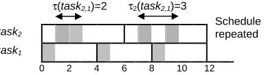
(22) 9.2 9.3 9.4 9.5 9.6. 9.7 9.8 9.9 9.10 9.11 9.12 9.13 9.14 9.15 9.16. 9.17 9.18. 9.19. Flexible timing constraints for control tasks Fixed timing constraints vs. flexible timing constraints (times in ms) Non-feasible schedule (in ms) Feasible schedule (in ms) Inverted pendulum response of a task scheduled using flexible timing constraints (either using compensations or not), which was not schedulable using fixed timing constraints. Inverted pendulum response error ITAE index depending on different instance separations (top) and response times (bottom) QoC of sequences of constant instance separations Instance separations sequences vs QoC Scheduling objective Offline construction (schedule repeated) Run time schedule (schedule repeated) Inverted pendulum response obtained by the control task in the offline schedule (dotted) or by the ordering produced by the online algorithm (solid) New run time schedule (schedule repeated) Inverted pendulum responses obtained by the control task in the ordering produced by the online algorithm whether new instances are added (solid line) or not (dotted line) during the LCM of the tasks periods Best effort algorithm Offline schedule (first row), optimum schedule (second row) and sub optimum schedule (third row) de-phasing and re-phasing found by the best effort algorithm. QoC improvement. 143 144 145 146 146. 148 150 151 152 154 157 157 158 159 159. 160 161. 163.

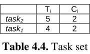
(23) List of Tables Table 2.1 Task set 2.2 Dispatcher table 2.3 Priority assignment for RM 2.4 Closed-loop system properties 3.1 Task set 3.2 Task set with two control tasks with strict harmonic period relation 3.3 Task set with two control tasks with soft harmonic period relation 4.1 Task set 4.2 Task set 4.3 Task set 4.4 Task set 4.5 Jitters summary for the partial RM schedule 4.6 Task set 4.7 Task set 4.8 Sampling interval (h(tasksfc,k)) variability (in ms) 4.9 Sampling-actuation delay (τ(tasksfc,k)) variability (in ms) 4.10 PID correct values vs. taskPID wrong values 7.1 Computational overhead 7.2 Memory requirements for the inverted pendulum 8.1 Task set 8.2 Sequence of sampling intervals and sampling-actuation delays due to scheduling inherent jitters (in ms) 8.3 Table for task taskCTsfc containing the parameters for the run time adjustment 8.4 Influence of different values for feasible sampling intervals on each performance loss criterion values tendency 8.5 Influence of different values for feasible sampling-actuation delays on each performance loss criterion values tendency 8.6 Absolute performance loss error due to EDF and RM 8.7 Sequence of sampling intervals and sampling-actuation delays due to scheduling inherent jitters 8.8 Performance values depending on the ordering of the jitter sequence 8.9 Performance study. Varying feasible sampling-actuation delays vs. a fixed time delay 9.1 Task set (in ms), where Ti, Ci, Di and Oi denotes period, computation time, deadline and offset 9.2 Task set (ms) 9.3 Achieved QoC for each scheduling strategy 9.4 Algorithm execution corresponding to the second row Figure 9.18 (top) and to the third row Figure 9.18 (bottom). Pg. 13 14 16 30 49 50 50 55 57 58 59 59 62 64 65 66 68 114 115 123 124 127 132 133 135 136 136 139 145 156 159 162.

(24)

(25) List of symbols Symbol taski taski,k Di Ti Ci ci Pi Oi U s(taski,k) f(taski,k) r(taski,k) h(taski,k) τ(taski,k) g y(t) u(t) r(t) e(t) x(t) tk ak h τ FHi FTi hi,j τi,j A B C D Φ Γ L K ωn ζ. Description Periodic task i, where i identifies the task kth instance (or invocation) of a periodic task taski Task taski relative deadline Task taski period Task taski worst case execution time Task taski exact execution time Task taski priority Task taski offset Processor utilization Start time of the kth instance of task taski Finishing time ot the kth instance of task taski Release time of the kth instance of task taski Sampling interval of the kth instance of the control task taski due to sampling jitter Sampling-actuation delay of the kth instance of the control task taski due to sampling-actuation jitter Basic time granularity length (in the system model) Output of a controlled process (system response) Input of a controlled process (control signal) Reference signal Closed-loop system error State vector Sampling instant Actuation instant Sampling period Time delay Set of feasible sampling intervals for a given control task taski Set of feasible sampling-actuation delays for a given control task taski Feasible sampling interval belonging to FHi, where i identifies the control task taski and j identifies the specific value Feasible sampling-actuation delay belonging to FTi, where i identifies the control task taski and j identifies the specific value Continuous-time system matrix Continuous-time input matrix Continuous-time output matrix Continuous-time direct matrix Discrete-time system matrix Discrete-time input matrix Discrete-time gain matrix Discrete-time observer matrix Natural frequency Damping ratio.

(26)

(27) List of acronyms Acronym AD DA DC EDF FPS GCD LCM PID QoC RM SFC WCET. Description Analogue-to-Digital Digital-to-Analogue Direct Current Earliest Deadline First Fixed Priority Scheduling Greatest Common Divisor Least Common Multiple Proportional, Integral and Derivative Quality-of-Control Rate Monotonic State Feedback Controller Worst-Case Execution Time.

(28)

(29) 1. Introduction. 1. Chapter 1 Introduction The objective of computer control is to use computers to manipulate the available inputs of a dynamic system in order to cause the system to behave in a manner more desirable than it otherwise would [LUE79]. Computer control is used in many application areas, such as factory automation, process control, robotics, automotive systems, and others. In such applications, computers are used to control processes, and are expected to react within precise time constraints to external events according to the application requirements. Computer control systems1 are expected to behave correctly both in the value and timing domains: they process inputs and provide the adequate outputs with an accurate timing. Computing systems in which meeting timing constraints is essential to correctness, i.e., their correctness depends not only on the logical results of the computations but also on the time at which these results are produced [STA88], are called real-time systems. Therefore, computer-controlled systems must be considered real-time systems. In real-time systems, by means of algorithms, task scheduling deals with the problem of meeting the timing constraints of the tasks. These timing constraints are derived from the application timing requirements. During the last three decades, real-time scheduling has been a very active research area and many different scheduling models and methods have been presented. Scheduling approaches are based on standard task timing constraints such as periods and deadlines [BUT97]. Computer-controlled systems theory assumes a highly deterministic timing of an implementation [AST97]. The classic mathematical models for computer-controlled systems transform a continuous-time system into a discrete-time system by considering the behaviour of the signals (measured and control signals) at the sampling instants only. That is, continuous-time signals are replaced by sequences of numbers, which represent the values of the signals at certain synchronised times. As a consequence, computers for control applications are expected to behave as the mathematical models demand. For that reason, the most stringent timing constraints for real-time systems have their origin in the timing requirements imposed by discrete-time control theory. The application of standard timing constraints for control tasks impairs system schedulability because those timing constraints, which are artificial constraints rather than constraints able to comply with the control timing requirements, over-constrain the schedule [FOH97]. On the other hand, real-time scheduling introduces variability in the starting and completion times of successive instances of a same task, i.e., jitters [BAR97]. The jitters inherent to scheduling for control tasks prevent controllers from fulfilling the control. 1. Also known as computer-controlled systems, sampled data systems or discrete-time systems [AST97]..

(30) 2. 1. Introduction. performance requirements, thus degrading the controlled system response. This degradation appears because these jitters in the control tasks violate the strict timing assumptions that discrete-time control theory imposes. In this thesis we present a flexible integrated scheduling and control analysis and design framework for real-time control systems that improves both system schedulability and controlled systems performance. We present a new controller design method for control tasks that takes scheduling inherent jitters into account, thus removing the control performance degradation that would otherwise occur. In addition, by exploiting the timing properties imposed by this new controller design method, we show how to derive more flexible timing constraints for control tasks. These allow us to obtain feasible schedules from task sets (including control and non-control tasks) that are not schedulable using traditional scheduling and control design methods, thus improving system schedulability. Finally, we formulate a novel scheduling problem, Quality-of-Control scheduling, in which improving both system schedulability and controlled systems performance is of main concern. Specifically, we show that the control performance information that can be associated to each control task timing constraint can be used to improve the performance of the controlled processes in the presence of perturbations.. 1.1 Motivation The development of real-time control systems is a complex task, requiring the integration and good understanding of both control and real-time systems theory. However, control theory and real-time scheduling theory have been relatively independent research areas [TOR98]. This fact arises from the traditional way real-time control systems have been developed; that is, differentiating two separate stages, each in isolation [SET96]: first, control design and then its computer implementation. This has allowed the control community to focus on its own problem domain without being really concerned about how the implementation is being done. The control community sees the computing platform as providing the determinism that discrete-time control theory requires. Control theory has considered implementation other than dedicated processors systems only to a very small extent. Consequently, when computing resources (processor time and communication bandwidth) are limited, control theory rarely advises on how to design controllers to take these limitations into account [ARZ00]. On the other hand, this has released the scheduling community from the need to understand what impact scheduling inherent jitters have on the stability and performance of control systems. Real-time scheduling generally assumes that a control algorithm implemented as a periodic task with standard timing constraints such as period and deadline will meet the control requirements (in terms of stability and control performance). However, since a periodic task execution in scheduling theory is an execution that takes place anywhere within its deadline, small time variations (i.e., jitters) occur at each task instance execution. Consequently, the resulting jitters for control task instances do not comply with the deterministic timing demanded by discrete-time control theory in the implementation. Specifically, as we show in this thesis, the negative effects of bringing together the separate results of control and scheduling theories for computer-based control systems are:.

(31) 1. Introduction. 3. •. Poor computing system schedulability: in general, when discrete-time control theory timing requirements are expressed with traditional periodic task timing constraints (periods and deadlines), the task set schedulability becomes unfeasible.. •. Controlled system performance degradation: scheduling inherent jitters for periodic control tasks (which implement controllers designed using classic2 discrete-time control theory) degrade the performance of the controlled system, and can even cause a critical failure (instability).. The integrated control and scheduling framework we present in this thesis bridges the gap between the two communities, joining control and scheduling theory so as to provide solutions to both problems.. 1.2 Objectives In the thesis we show how to use a combination of control and scheduling principles in order to design controllers that deal with new and more flexible timing constraints and to allow scheduling approaches to take scheduling decisions considering both system schedulability and control performance. Specifically, we demonstrate that combining offline scheduling analysis and offline control analysis with online scheduling and dynamic control compensations we obtain better system schedulability, and better control performance. The integrated control and scheduling framework that we present as an analysis and design methodology for real-time control systems is based on two novel paradigms: •. Flexible control design: we present a new controller design method, compensation approach, that goes beyond the classic discrete-time control theory timing assumptions of equidistant sampling and equidistant actuation given by the constant sampling period and constant time delay specified at the design stage. Instead of specifying a single value for the sampling period and a single value for the time delay, we design controllers to account for a set of feasible sampling intervals and for a set of feasible sampling-actuation delays. This controller design method, which includes new stability and response analysis, relies on the idea of adjusting controller parameters at runtime (compensations) according to the specific implementation timing behaviour, i.e., scheduling inherent jitters. In addition, design decisions are also taken regarding implementation details such as space and time overheads. We consider two alternatives: (a) performing the compensation calculations online - if these incur only negligible overheads - or (b) determining offline the compensation parameters for table look-up at runtime. We characterise when each of these alternatives is suitable.. •. Flexible control task scheduling: we present new flexible timing constraints for control tasks. Controllers based on the compensation approach assume a closed-loop implementation with irregular sampling and varying time delays. The new timing assumptions behind the compensation approach give the potential to derive more. 2. Classic discrete-time control theory refers generically to well known discrete-time control methods and models based on regularly sampled discrete-time systems (regardless of whether they belong to classical or modern control theory, a distinction made within the control community to differentiate methods based on transfer function or state-space models. See section 2.2.1 for further details)..

(32) 4. 1. Introduction. flexible timing constraints for control tasks, beyond task periods and deadlines necessary to apply standard periodic task scheduling. Control tasks are no longer seen as classic real-time tasks with fixed values assigned to their timing constraints (such as periods and deadlines). They are characterised by flexible timing constraints in terms of feasible instance separation and feasible response time sets. That is, at each control task instance execution, scheduling approaches can choose for the instance separation and response time constraints different values from these sets, taking into account, for example, schedulability of other tasks or performance improvement of the controlled processes. These constraints are defined on a per control task instance basis, as opposed to fixed values, such as periods and deadlines, applicable to all instances – as assumed by standard scheduling schemes such as Rate Monotonic (RM) [LIU73], Earlier Deadline First (EDF) [LIU73] and Fixed Priority Scheduling (FPS) [TIN94]. Thus, our methods provide more flexibility than the one obtained by using fixed timing constraints. Using these novel paradigms, we show how to solve the two problems outlined in the previous section: •. With the flexibility given by the compensation approach controller design method, we eliminate the control performance degradation that control tasks subject to scheduling inherent jitters introduce in the controlled processes. Although the scheduling community has tried to minimise jitters by designing specific purpose real-time task models and algorithms, jitter is an inherent scheduling problem and cannot be completely removed. Nevertheless, we show that by accepting jitters in the control design, control task implementing controllers designed with the compensation approach solve the degradation that would otherwise occur. In summary, we solve the problems posed by scheduling inherent jitters for periodic control tasks, which in general are not addressable using traditional offline and online scheduling based approaches nor by previous real-time and control integration approaches.. •. With the new flexible timing constraints for control task scheduling we provide the instruments that can be used to transform unfeasible schedules and instable control systems into feasible schedules and stable control systems. The application of fixed timing constraints for control tasks impairs system schedulability by over-constraining the schedule. However, the compensation approach affords us the possibility of relaxing the strict periodicity and deadline requirements for traditional control task scheduling (based on fixed timing constraints); instead, we demonstrate how we can take advantage of the new flexible timing constraints for control tasks scheduling in order to improve system schedulability. Note that we do not propose a specific scheduling approach, rather a new set of flexible control timing constraints for control tasks that we show can be used to achieve stable control systems when the same control tasks characterized by fixed timing constraints were not schedulable.. In addition, by taking advantage of the compensation approach and flexible timing constraints for control tasks, we define a Quality-of-Control (QoC) metric that associates with each feasible flexible timing constraint a quantitative value expressing control performance in terms of the controlled system error resulting from the use of that timing constraint. This offers the possibility of taking scheduling decisions at each control task.

(33) 1. Introduction. 5. instance execution considering this control information, thus demanding novel scheduling approaches. We present a new scheduling paradigm, QoC scheduling, in which we demonstrate that the QoC information of task timing constraints can be used to improve the performance of the controlled processes in the presence of perturbations. After formulating the QoC scheduling problem, we categorise the main scheduling issues and identify feasible solutions. Specifically, we show how the problem of reacting to perturbations with control tasks specified with control timing constraints expressing QoC can be achieved applying standard guarantee techniques. 1.3 System model In this section we describe the system model for the approach to scheduling and control codesign we present. We consider a distributed control system that consists of a set of processing nodes that run one or several tasks, some of them in charge of controlling physical systems (plants/processes), which communicate data across a communication network. See Figure 1.1 for a full view of the system model. Planta. Plantb. Node1. Plantc. Node2. Node3. Noden. Network. Figure 1.1. System model scheme. We assume a discrete time model [KOP92]: An external observer counts the ticks of the globally synchronized clock (which is based on the metrics of the physical second, as a time unit) with granularity of length g and assigns natural numbers from 0 to ∞ to them. All the nodes and the communication network of the system have the same time granularity. Digital-to-Analogue (DA) and Analogue-to-Digital (AD) converters (that interface processing nodes and the continuous-time physical systems that are controlled) have the same time granularity. We assume that the DA and AD operation times are negligible compared to g (granularity length). At a node level, each node runs a set of tasks. We distinguish two types of tasks according to their functionality: control tasks and non-control tasks. Control tasks are in charge of controlling the physical systems (through measuring the controlled variables, y(t), and transmitting the control signals, u(t)), if any. A physical system is controlled by one or several control tasks. Non-control tasks are the remaining tasks. See Figure 1.2 for an illustrative scheme of the node level. Planta. ya(t). ua(t) Task2. ub(t). Task4. Task1 Task5. Plantb Task6. Task3. Figure 1.2. Node level scheme. yb(t).

(34) 6. 1. Introduction. In a node, at the operating system level, a dispatcher (also called scheduler), at each time it is invoked, either assigns a task to the processor or leaves it idle. A task is executed uninterruptedly during the granularity length g. The task execution lengths are a multiple of the granularity. We regard the actual time to perform the dispatching and the task context switching to be negligible with respect to g3. If the dispatching and the task context switching are too long, it can be included in the worst-case execution time of the task. The allocation of tasks to processors is carried out using any of the allocation published methods, such as in [FOH95] or [RAM90]. Therefore, the scheduling strategies we present are in a node level context.. 1.4 Thesis structure The thesis is organized as follows: Chapter 2 gives a brief overview of basic but important concepts of both real-time and control systems theory and practice. Also, the state of the art concerning this thesis is reviewed. In Chapters 3 and 4 we identify the two main problems this thesis solves. In Chapter 3 we explore the impact of classic control timing requirements on real-time scheduling. We show that in general this leads to unfeasible scheduling scenarios. Chapter 4 explains the impact of scheduling inherent jitters on control tasks. We show that jitters in control task instance executions degrade the controlled system response, even causing instability. In Chapter 5 we discuss the necessity of developing a) new flexible control design methods and b) more flexible timing constraints for control task scheduling for solving the problems identified in the previous two chapters. In Chapter 6 we define the compensation approach controller design method. We discuss its completeness in terms of coping with all possible closed-loop implementations. We then formulate the new controller design method problem based on state-space models. After the problem formulation, in Chapter 7 we present the new controller design method that includes new stability and response analysis, all based on state-space models. We also address practical aspects such as code implementation details and different strategies for the controller parameter adjustment required for the application of the compensation approach. In Chapter 8 we explain the use of the compensation approach as a control-based solution to eliminate the degradation that scheduling inherent jitters introduce in the controlled system response. In this context, we also present a performance evaluation of the application of the compensation approach. In Chapter 9 we present new flexible timing constraints for control task scheduling: firstly we demonstrate how to use them to obtain feasible schedules of task sets that were not feasible using fixed timing constraints; secondly, after presenting the QoC metric and 3. For example, in the real-time kernel S.Ha.R.K. (Soft and Hard Real-time Kernel) [GAI01], the task context switch and dispatcher execution is 15µs. We regard such times for our system model negligible because the granularity we use is of the order of milliseconds..

(35) 1. Introduction. 7. formulating the QoC scheduling problem, we demonstrate that scheduling decisions can be taken accounting for both schedulability and control performance improvement. Finally, Chapter 10 draws the conclusions of this thesis, lists the main contributions and points out directions for future work. At the end all references are listed. We also include three appendices: Appendix A with code details of the controllers we design and use, Appendix B with a numerical stability analysis of two of the examples we use and Appendix C with the closed loop matrices we found in the system evolution for one of the examples we use..

(36)

(37) 2. Background and state of the art. 9. Chapter 2 Background and state of the art The successful design and implementation of real-time control systems requires the interaction between two technical disciplines: real-time systems and control systems. However, as pointed out in [TOR98], control theory and real-time theory have been relatively independent research areas. The aim of this chapter is to provide a brief overview of basic but important concepts of both real-time and control systems theory and practice. In this way, we introduce the fundamental ideas for understanding the integrated control and scheduling framework we present while bridging the existing gap between both real-time and control communities. In this chapter we also review related work. We show that the practical problems posed by: a) scheduling inherent jitter in control tasks, i.e., controlled system degradation, b) fixed timing constraints to meet the stringent timing requirements assumed by discrete-time control theory, i.e., poor system schedulability, have not been formally addressed. In addition, neither controlled systems performance nor system schedulability have been, in any of the previous works, jointly improved as we do with the application of more flexible controller designs and more flexible timing constraints for control tasks scheduling.. 2.1 Real-time systems Real-time systems can be constructed out of sequential programs, but are typically built from concurrent programs, called tasks. A real-time task is an executable entity of work that, at a minimum, is characterized by a worst-case execution time (WCET) [PUS89] and a time constraint [RAM96]. The WCET is an estimation of the maximum time required by the processor to execute the task. A typical timing constraint on a real-time task is the relative deadline, i.e. the time interval within which the task must complete its execution. The objective of real-time computing is to meet the individual timing constraints of tasks. Realtime systems are computing systems in which the correctness of the computations depends not only on the logical results but also on the time at which the results are produced [STA88]. These systems have a unique set of requirements that are not always taken into consideration, leading to serious misconceptions about real-time computing [STA88]. The main objective of real-time computing is not fast computing, it is predictability [STA90]. The fast computing objective is to minimize the average response time of a given set of tasks. Predictability implies that it has to be possible to prove that timing requirements are met, in accordance to system specifications. Regarding timing requirements, real-time scheduling is the main concern..

(38) 10. 2. Background and state of the art. In real-time systems, scheduling theory addresses, by means of algorithms, the problem of meeting the specified timing requirements in order to have understandable and predictable system timing behaviour. Therefore, scheduling involves the allocation of resources and time in such a way that certain performance requirements are met [RAM94].. 2.1.1 Tasks constraints Real-time tasks are computing entities that must process inputs and provide the adequate outputs (see Figure 2.1) within a time interval, i.e. relative deadline, which is dictated by the requirements of the application. Read input Perform computatoin Write output. Figure 2.1. Task structure Depending on the consequences of a missed deadline, real-time tasks can be characterized according to its criticality as: •. Hard real-time tasks: the completion of the task must be within its deadline, otherwise serious consequences occur.. •. Soft real-time tasks: a task is soft if missing its deadline decreases the performance of the system but no serious consequences occur if there is a late completion.. Accordingly, although we can differentiate two types of real-time systems, hard and soft, many systems consist of both hard and soft real-time tasks. Sometimes, if the consequences of missing a deadline are catastrophic, the target system is called a critical (or safetycritical) real-time system instead of a hard real-time system. In fact, it has to be pointed out that there is a current debate on the previous definitions. Another timing characteristic that can be specified in a real-time task concerns the regularity of its activation. Depending on this, a task is defined as a periodic, aperiodic and sporadic. Periodic tasks consist of a sequence of identical activities, called instances, which are recurrently activated on a regular basis. We denote the kth instance of a periodic task taski by taski,k. Figure 2.2 shows an example of tasks instances for a periodic task. Ti Di. Kth Instance Ci. taski (k-3)Ti. (k-2)Ti. (k-1)Ti. kTi. time. Figure 2.2. Sequence of instances for a periodic task The activation of the kth instance of a periodic task taski is given by (k-1)Ti, where Ti is called the period of the task. In many practical cases, a periodic task taski can be completely characterized by its WCET Ci (which is an estimation of the maximum time required by the.

(39) 2. Background and state of the art. 11. processor to execute the task), its relative deadline Di (which is the time interval within which the task should be completed), which is often considered to coincide with the end of the period. On the other hand, a task that is not invoked at regular intervals is an aperiodic task. Aperiodic tasks characterized by a minimum inter-arrival time are called sporadic. For further details on tasks characterization, see for example [BUT97]. Standard timing constraints for a periodic task (such as period and deadline) are fixed, i.e. a single value holds for all instances of the task [FOH94]. We have to point out that some works, for example [DOB01], distinguish between simple constraints, i.e. period and deadlines, and complex constraints such as end-to-end deadlines. We do not make this distinction. For a discussion on task constraints, see [RAM96]. Other typical constraints that can be specified in real-time tasks, apart from timing constraints, are precedence relations and resource constraints. Precedence constraints refer to the fact that computational activities cannot be executed in arbitrary order but have to respect some precedence relations defined at the design stage. Resource constraints refer to the fact that computational activities that share resources have to be synchronized.. 2.1.2 Real-time Scheduling When a processor has to execute a set of concurrent tasks, the processor has to be assigned to the various tasks according to a predefined criterion, called a scheduling policy. There are a great variety of algorithms proposed for scheduling of real-time systems today. A schedule is an assignment of tasks to the processor, so that each task is executed until completion. The dispatcher allocates the processor to the task selected by the scheduling policy. Consequently, a task that could potentially be executed by the processor (active task) can be either in execution (running task) or waiting (ready task) in the ready queue if another task is executing. Context switches allow the running task exchange on the processor. In this context, we introduce the following notation to facilitate the description of schedules (and scheduling policies): r(taski,k). denotes the release time of the kth instance of task taski, i.e. the time at which a task instance becomes ready for its execution. s(taski,k). denotes, the start time of the kth instance of task taski, i.e. the time at which a task instance starts its execution. f(taski,k). denotes the finishing time (also called completion time) of the kth instance of task taski, i.e. the time at which a task instance completes its execution. In Figure 2.3, these concepts are portrayed. Ti taski. taski,k r(taski,k). s(taski,k). f(taski,k). Figure 2.3. Task instance description. time.

(40) 12. 2. Background and state of the art. As described in [BUT97], in general, to define a scheduling problem we need to specify three sets: a set of tasks, a set of processors and a set of types of resources. Moreover, precedence relations among tasks can be specified through a direct acyclic graph, and timing constraints can be associated with each task. In this context, scheduling means to assign processors and resources to tasks in order to complete all tasks under the imposed constraints. This problem, in this general form, has been shown to be NP-complete [GAR79] and hence computationally intractable. Note that the complexity of scheduling algorithms is highly relevant when scheduling decisions must be taken on-line, during task execution. In order to reduce the complexity of constructing a feasible schedule, one may simplify the computer architecture (e.g., by restricting it to the case of uniprocessor systems), or may make simplifying assumptions on the tasks (e.g., remove precedence constraints). A schedule is said to be feasible if all tasks can be completed according to a set of specified constraints. In order to check the feasibility of the schedule before tasks execution, the system has to plan its actions by looking ahead to the future and by assuming a worst-case scenario. Recall that in hard real-time applications that require highly predictable behaviour, the feasibility of the schedule should be guaranteed in advance, that is, before tasks execution. Feasibility tests (see [JEF93] for further discussion) can be based on the processor utilization approach (which measures the fraction of processor time spent in the execution of the task set) and/or on response time analysis techniques [JOS98] (which uses recurrent formulas to calculate the worst-case finishing time of any task). For example, a necessary condition for achieving schedulability using the processor utilization (U) approach on a single processor is given by (2.1). n. Ci. ∑T i =1. ≤1. (2.1). i. where Ci and Ti are the task taski worst-case execution time and period, respectively. Known sufficient schedulability conditions for scheduling algorithms such as RM and EDF [LIU93] are given by (2.2), where U=1 for EDF and U=n(21/n-1) for RM. n. Ci. ∑T i =1. <U. (2.2). i. In the following, we give a short description of the main types of scheduling algorithms (this classification is based on the assumptions made about the system or the tasks). Rather than providing an exhaustive description, we pick up the most important concepts and properties that are of special interest for the work of this thesis. Offline vs. online scheduling Among the great variety of real-time scheduling approaches that have been presented, realtime scheduling algorithms fall into two categories [STA95], depending on the time scheduling decisions are taken: offline and online scheduling..

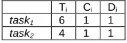
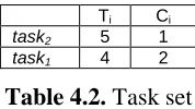
(41) 2. Background and state of the art. 13. In offline scheduling, the scheduler has complete knowledge of the task set and its constraints, such as deadlines, computation times, precedence constraints and so on. The schedule construction is based on fixed parameters, assigned to tasks before their activation. The entire offline guaranteed schedule is stored in a table (which contains all guaranteed tasks arranged in the proper order) and dispatched later during system runtime. The main advantage of offline scheduling is that it provides determinism, as all times for task executions are determined and known in advance. In addition, the runtime overhead does not depend on the complexity of the algorithm. This allows very sophisticated algorithms to be used to solve complex problems (e.g., control constraints). However, as all actions have to be planned before startup, run-time flexibility is lacking. Offline scheduling is also referred as static or pre-runtime scheduling. In contrast, online scheduling algorithms make their scheduling decisions at runtime. Online schedulers are flexible and adaptive, but they can incur significant overheads because of runtime processing. Besides, online scheduling algorithms do not need to have complete knowledge of the task set or its timing constraints. For example, with an external event that arrives at the runtime of the system, we need to deal with it upon its arrival. In online scheduling algorithms, scheduling decisions are taken every time a new task enters the system, when a task becomes ready and/or when a running task terminates. Although online scheduling can provide more flexibility, it is limited with respect to predictability, as actual start and completion times of execution depend on run-time events. It is worth noting that depending on the algorithm, the guarantee must be done on-line (e.g., when a new task enters the system). In such cases, since the guarantee algorithm is based on worst-case assumptions, a task could be unnecessarily rejected. On the other hand, the benefit of having an online guarantee mechanism is that a potential overload situation can be detected in advance, thus avoiding negative effects on the systems. Online scheduling is often referred to as dynamic or runtime scheduling. These are also scheduling approaches that fall into both categories. For example [FOH95] combines offline and online scheduling, taking advantage of the determinism provided by offline scheduling, and the flexibility provided by online scheduling. To illustrate the determinism provided by offline and online scheduling policies in terms of knowing the exact task executions times before run-time, consider the following task set (Table 2.1) with two periodic tasks, where Ti is the task period and Ci is the WCET. We assume deadlines equal to periods.. task2 task1. Ti 5 4. Ci 2 1. Table 2.1. Task set Applying an offline scheduling strategy, we can construct, according to task timing constraints, the feasible offline schedule over the tasks periods LCM (Least Common.

(42) 14. 2. Background and state of the art. Multiple)1 that we show in Figure 2.4 (where boxes mark task periods and shaded areas mark worst-case execution times). Repeated schedule. task2 task1. time 0. 1. 2. 3. 4. 5. 6. 7. 8. 9. 10. 11 12 13 14. 15 16 17 18 19 20. Figure 2.4. Offline schedule Given this offline schedule, at run time, the dispatcher will execute task instances (taski,k) according to the ordering provided by the constructed table (Table 2.2) for each LCM. Time Task instance. 0 task2,1. 2 task1,1. 4 task1,2. 5 task2,2. 8 task1,3. 10 task2,3. 12 task1,4. 15 task2,4. 17 task1,5. Table 2.2. Dispatcher table Therefore, looking at the schedule (Figure 2.4) and dispatcher table (Table 2.2), at run time, the execution start time of each instance will coincide with the offline instances start times. However, looking at the completion times, since the offline schedule is based on worst-case execution time, the run time completion times may be different to the offline completion times, because at run time, each task instance can execute less than the assumed worst-case (as we show in Figure 2.5 for one of the LCM executions, where shaded areas mark now actual execution times). task2 task1. time 0. 1. 2. 3. 4. 5. 6. 7. 8. 9. 10. 11 12 13 14. 15 16 17 18 19 20. Figure 2.5. Run time execution of the offline schedule of Figure 2.4 Note for example that the first, third and fourth instances of task task2 (starting at times 0, 10 and 15 respectively, Figure 2.5) executes less than its WCET. Instead of executing for 2 time units (as assumed by the worst case scenario, Table 2.1), the first and third instances execute 1 time unit while the fourth instance executes 1.5 time units. Similar phenomena occur in the finishing times of instances of task task1 (Figure 2.5) Therefore, although the starting times of each task instance is known before run time, the actual finishing times, if the offline schedule is constructed in terms of the tasks WCET, may not coincide with the offline finishing times. However, if what characterises each task (in Table 2.1) is the exact execution time (which is a reasonable assumption for most real-time control systems [BUT98]) instead of the worstcase execution time, the run time completion times will also coincide with the offline completion times. 1. Although theoretically, offline scheduling can construct non-periodic schedules, for practical purposes, offline schedules are constructed over the LCM of the task’s periods, which implies a LCM periodic pattern..

(43) 2. Background and state of the art. 15. However, none of these properties (known start and completion times) apply to online scheduling. For example, we apply EDF [LIU73] to the task set specified in Table 2.1. Recall that EDF is an online scheduling policy where tasks instances are dispatched at run time according to the earlier deadline. The set of tasks complies the EDF schedulability test (2.2) as detailed in (2.3). 2. U =∑ i =1. Ci 2 1 = + = 0.65 ≤ 1 Ti 5 4. (2.3). An example of the schedule that we obtain over the tasks periods LCM is shown in Figure 2.6, where boxes mark task periods and shaded areas mark WCET. Repeated schedule. task2 task1. time 0. 1. 2. 3. 4. 5. 6. 7. 8. 9. 10. 11 12 13 14. 15 16 17 18 19 20. Figure 2.6. Example of schedule produced by EDF In this case, at run time, every time a task instance terminates its execution (which can execute its worst execution time or less), the scheduler assigns the processor to another task instance. Consequently, before run time, the exact start and completion times of each task instance is not known. The previous problem (knowing task start and completion times before run time) increases when the online scheduling policy takes scheduling decisions upon arrival of aperiodic or sporadic tasks. Pre-emptive vs. non pre-emptive Looking at the run-time behaviour of different scheduling policies, two modes can be distinguished: pre-emptive and non pre-emptive scheduling. With pre-emptive scheduling, the running task can be interrupted at any time by another task, according to some predefined scheduling policy. In non pre-emptive scheduling, a task, once started, is executed by a processor until its completion. When the application tasks have different levels of criticalness expressing task importance, i.e., priority, pre-emption permits us to anticipate the execution of the most critical tasks, producing more efficient schedules in terms of system responsiveness. However, this also implies that predictability in terms of knowing times for task executions decreases. To illustrate the decrease of determinism that pre-emptive scheduling policies implies in terms of knowing task executions times before run-time, we again consider the task set we used before (Table 2.1). For example, we apply to the task set RM [LIU73] scheduling approach, which is a pre-emptive scheduling policy based on the following priority assignment scheme: to give the tasks a priority level based on its period: the smaller the period, the higher the priority; that is, Ti < Tj, Pi > Pj, where Ti and Pi denotes the task period and priority of each task taski. Table 2.3 also gives the priority assignment for the task set we are considering (recall that task deadlines are assumed to be equal to task periods)..

(44) 16. 2. Background and state of the art. Ti 5 4. task2 task1. Ci 2 1. Pi 2 1. Table 2.3. Priority assignment for RM The set of tasks complies with the RM schedulability test (2.2) as detailed in (2.4) 2. U =∑ i =1. Ci 2 1 = + = 0.65 < 2( 21 / 2 − 1) ≈ 0.83 Ti 5 4. (2.4). An example of the schedule that we obtain over the tasks periods LCM is shown in Figure 2.7, where boxes mark task periods and shaded areas worst-case execution times. Repeated schedule. task2 task1. time 0. 1. 2. 3. 4. 5. 6. 7. 8. 9. 10. 11 12 13 14. 15 16 17 18 19 20. Figure 2.7. Example of schedule produced by RM As can be seen in Figure 2.7, the fourth instance of task task2 is pre-empted at time 16 by the fifth instance of task task1. This interruption adds more variability in the completion time of the fourth instance of task task2. Time triggered vs. event triggered There are two fundamentally different principles that determine the activation of tasks in a real-time system, event-triggered and time-triggered. In event-triggered systems, all activities are activated in reaction to relevant events external to the system. When a significant event in the outside world happens, it is detected by some sensor, which then causes the attached device (processor) to get an interrupt signal. For soft real-time systems with lots of computing power to spare, this approach is simple, and works well. The main problem with event-triggered systems is that they can fail under heavy load conditions, i.e., when many events are happening at once. Event-triggered designs give a faster response at low load but more overhead and chance of failure at high load. This approach is more suitable for dynamic environments, where dynamic activities can arrive at any time. In a time-triggered system, all activities are activated at certain points in time that are known a priori. Accordingly, all nodes in time-triggered systems have a common notion of time, based on synchronised clocks. One of the most important advantages of time-triggered systems is the deterministic temporal behaviour of the system, which eases system validation and verification considerably. Time-triggered systems are suitable in static environments in which the system behaviour can be completely known in advance. Summary As we have seen in the previous scheduling examples, as far as task timing constraints are fulfilled, the periodic task execution given by scheduling theory is an execution that takes place some time within the task relative deadline. This has the effect of introducing start-.

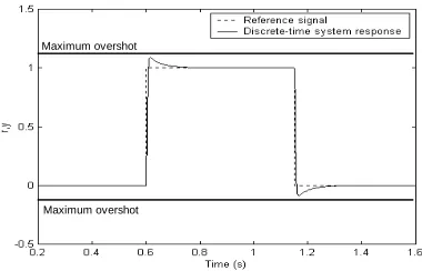
(45) 2. Background and state of the art. 17. time delays in task instance executions, as well as introducing variable completion times. We call the variability caused by scheduling policies on task instance executions scheduling inherent jitters. Although a great variety of scheduling policies have been presented (for handling periodic, aperiodic and sporadic tasks, on a single and multiprocessor architecture, with simple and complex constraints, etc) in this work we will mainly focus on offline constructed schedules as well as traditional Earliest Deadline First (EDF) [LIU73] and Fixed Priority Scheduling (FPS) [TIN94] based scheduling approaches. The main reason is that if the methods we present work well for these standard approaches, they should improve further if applied to more sophisticated scheduling algorithms based on the former. Note that in the following chapters, we do not propose any scheduling algorithm. Rather, we provide instruments to be used to improve the controlled systems responses and system schedulability, which we show to be applicable to standard scheduling approaches. This explains why we will not compare any scheduling algorithms. In this section, specific features and types of scheduling algorithms have been described. For further reading, see [SHI94], [AUD95], [BUR97], [BUT97], [TIN97] and [STA98].. 2.2 Control systems A control system is an interconnection of components forming a system configuration that will provide a desired system response [DORF95]. The basis for analysis of a system is the foundation provided by linear system theory, which assumes a cause-effect relationship for the components of the systems. A component or process to be controlled (also called physical system or plant) can be represented by a block (as shown in Figure 2.8) where the input-output relationship represents the cause-effect relationship. Input. Process. Output. Figure 2.8. Process to be controlled In control terms, the controlled variable is the quantity or condition that is measured and controlled (i.e., process output). The manipulated variable is the quantity or condition (i.e., process input) that is varied by the controller so as to affect the value of the controlled variable. Depending on the type of information that the controller uses to vary the manipulated variable, we distinguish between open-loop control and closed-loop control. The defining feature of an open-loop control is that the controller function that varies the manipulated variable is determined completely by an external process that accounts only for the desired output response (Figure 2.9) Desired output response. Controller. Input. Process. Output. Figure 2.9. Open-loop (also called feedforward) control system.