1
Universitat Politecnica de Catalunya
Tesi doctoral
Analysis of night-time climate in
plastic-covered greenhouses
Davide Piscia
2
Analysis of night-time climate in
plastic-covered greenhouses
Davide Piscia
Tesi Doctoral
Presentada al
Departament de Màquines i Motors Tèrmics
E.T.S.E.I.A.T.
Universitat Politecnica de Catalunya
Per a optar al grau de Doctor
3
Director de la tesis:
Doctor Juan Ignacio Montero
Ponente de la tesis:
4 Acta de qualificació de tesi doctoral Curs acadèmic:
Nom i cognoms
DNI / NIE / Passaport
Programa de doctorat
Unitat estructural responsable del programa
Resolució del Tribunal
Reunit el Tribunal designat a l'efecte, el doctorand / la doctoranda exposa el tema de la seva tesi doctoral titulada __________________________________________________________________________________________ _________________________________________________________________________________________. Acabada la lectura i després de donar resposta a les qüestions formulades pels membres titulars del tribunal, aquest atorga la qualificació:
APTA/E NO APTA/E
(Nom, cognoms i signatura)
President/a
(Nom, cognoms i signatura)
Secretari/ària
(Nom, cognoms i signatura)
Vocal
(Nom, cognoms i signatura)
Vocal
(Nom, cognoms i signatura)
Vocal
______________________, _______ d'/de __________________ de _______________
El resultat de l’escrutini dels vots emesos pels membres titulars del tribunal, efectuat per l’Escola de Doctorat, a instància de la Comissió de Doctorat de la UPC, atorga la MENCIÓ CUM LAUDE:
SI NO
(Nom, cognoms i signatura)
Presidenta de la Comissió de Doctorat
(Nom, cognoms i signatura)
Secretària de la Comissió de Doctorat
5
Ringraziamenti
Desidero ringraziare in primo luogo il dottor Juan Ignacio per il suo
inestimabile aiuto e supporto, e per avermi dato l’occasione di svolgere
questo lavoro di ricerca. Questi anni mi hanno insegnato il valore della
precisione, della metodologia e della scienzia.
Voglio ringraziare il Professore Oliva per la comprensione e l’ospitalitá (
nel programma di dottorato da lui diretto).
Ringrazio il Dottor Bailey per l’aiuto nella fase di redazione degli articoli, e
per non avermi mai denunciato alle autoritá inglesi per le mie frasi
contorte scritte in un ipotetico inglese.
Ringrazio inoltre i colleghi di lavoro che ho trovato e tuttora trovo nel
dipartamento di ingegneria dell’orticultura, Pere, Assuncio, le Marte,
Montze, Ileana, Jorge, Pepe y Mari Carmen.
Ringrazio l’IRTA e l’INIA che mi hanno fornito i mezzi e i servizi per
6
Summary
This work studied night-time greenhouse climate. The focus was on unheated plastic greenhouses and analyses were carried out using CFD models, Energy balance (ES) models and experimental data. The aims were twofold: on the one hand, it was intended to analyse and understand night-time greenhouse climate and propose solutions to the high-humidity issue. On the other hand, the aim was to investigate novel simulation approaches based on the coupling of CFD and ES models as well as the use of optimisation algorithms to study greenhouse climate.
Chapter 1 is an introductory chapter which includes the general context and overall research
objectives. Chapter 2 studies night-time climate in single-layer greenhouses by means of CFD. The model is validated and condensation User Defined Function (UDF) is introduced which accounted for the condensation rate found on the inner face of the greenhouse cover. Chapter 3 studies a commonly used solution to the issue of low night-time temperature. A
7
Resumen
Este trabajo analiza el clima nocturno del invernadero. EL objeto del estudio es el invernadero de plástico sin calefacción, cuyo clima se estudia utilizando modelos CFD, modelos basados en los balance de energía (ES) y s datos experimentales. El fin es doble, por un lado se trata de analizar y comprender el clima nocturno del invernadero, y proponer soluciones a los problemas relacionados con las altas tasas de humedad. Por otro lado se investigan nuevos métodos de simulación del clima del invernadero, métodos basados en el uso conjunto o acoplamiento de modelos CFD y ES , y también basados en la técnica de optimización.
8
Table of contents
1 Introduction ... 11
1.1 Foreword ... 11
1.2 The issue of low temperature and high humidity ... 11
1.3 Models for greenhouse climate simulations ... 12
1.3.1 CFD ... 13
1.3.2 Energy balance models ... 14
1.4 Research objectives ... 15
1.5 Thesis outlines ... 15
1.6 References ... 16
2 A CFD greenhouse night-time condensation model ... 18
2.1 Abstract ... 18
2.2 Nomenclature ... 19
2.3 Introduction ... 21
2.4 Material and Methods... 24
2.4.1 CFD simulation ... 24
2.4.2 Greenhouse measurements ... 28
2.5 Results ... 29
2.5.1 Model validation ... 29
2.5.2 Steady state CFD simulations ... 31
2.5.3 Transient analysis of the night-time greenhouse climate ... 34
2.6 Discussion ... 40
2.7 Conclusions ... 42
2.8 Appendix ... 42
2.9 References ... 44
3 A night time climate analysis of a screened greenhouse based on CFD simulations ... 48
9
3.2 Nomenclature ... 49
3.3 Introduction ... 50
3.4 Materials and methods ... 53
3.4.1 Computational fluid dynamics simulation ... 54
3.4.2 Greenhouse measurements ... 57
3.5 Results ... 58
3.5.1 CFD Model Validation ... 58
3.5.2 Climate analysis of the screened greenhouse ... 65
3.5.3 SC Transient climate analysis ... 69
3.5.4 Comparison of screened and single layer greenhouses ... 72
3.6 Discussion ... 74
3.7 Conclusions ... 77
3.8 References ... 78
4 A new optimization methodology used to study the effect of cover properties on night-time greenhouse climate. ... 80
4.1 Abstract ... 80
4.2 Nomenclature ... 80
4.3 Introduction ... 82
4.4 Material and methods ... 85
4.4.1 Simulations ... 85
4.4.2 Experimental greenhouse ... 90
4.5 Results ... 91
4.5.1 Validation of ES ... 91
4.5.2 ES simulation ... 93
4.5.3 CFD simulations ... 98
4.6 Discussion ... 101
4.7 Conclusions ... 103
10
4.9 References ... 106
5 A method of coupling CFD and Energy Balance models and their use to study humidity control in unheated greenhouses ... 110
5.1 Abstract ... 110
5.2 Nomenclature ... 110
a constant associated to the inner cover heat transfer coefficient... 110
5.3 Introduction ... 112
5.4 Material and methods ... 115
5.4.1 CFD model ... 116
5.4.2 ES model ... 119
5.5 Results ... 120
5.5.1 CFD ventilation rate parametric study ... 120
5.5.2 CFD convective coefficients rate parametric study ... 122
5.5.3 ES parametric study... 124
5.6 Discussion ... 130
5.7 Conclusions ... 132
5.8 Appendix ... 132
5.9 References ... 133
6 Conclusions ... 137
6.1 Final conclusions ... 137
6.2 General conclusion ... 139
6.3 Additional comments ... 140
11
1
Introduction
1.1
Foreword
The present challenge for the greenhouse industry is to provide an environment which is optimal for crop development. A greenhouse provides protection against insects, pests and extreme climate conditions such as heavy rain, strong winds and low temperatures.
According to recent studies (Giacomelli, Castilla, Van Henten, Mears, & Sase, 2008), there are more than 692,350 ha of plastic greenhouses in the world (48,250 ha of glasshouses), of which plastic greenhouses cover about 140,000 ha in Western Europe. Most Western European plastic greenhouses are located in coastal areas of Southern Europe, where the air temperature and solar radiation are higher than in Northern Europe. Under favourable outside air conditions, plastic covered greenhouses are fairly simple and offer little climate control. During hot periods, greenhouse climate is essentially controlled by means of natural ventilation (Baeza, Pèrez-Parra, Montero, Bailey, Lòpez, & Gàzquez, 2007). During cold periods, there is no means of climate control since the majority of plastic greenhouses are unheated.
1.2
The issue of low temperature and high humidity
A lack of available heating devices makes regulating greenhouse climate a significant problem. Indeed, during the cold season, night-time greenhouse climates are typified by low temperatures, high humidity and condensation.
12 In greenhouses the humidity regime is the result of the water vapour balance between different sources, such as plant transpiration and soil evaporation, and sinks, such as ventilation, dehumidification and condensation.
One of the terms in the mass balance equation for water vapour that has received least attention is condensation, possibly because it is difficult to measure the condensed water in a greenhouse, but also because most commercial CFD packages do not explicitly include a calculation for condensation rate. Nevertheless, roof condensation is an important sink for air humidity, particularly in unheated greenhouses under clear-night sky conditions, when the cover is usually the coldest part of the greenhouse.
High humidity and low temperatures are intrinsically related; indeed, an indirect way to reduce high humidity is to increase greenhouse temperature. In this respect, one technique commonly used to increase night-time temperature is to use a thermal screen. Since the 1970s, screens of different types have been used to conserve energy in heated greenhouses. During the period 1978 to 1988, scientific literature particularly addressed to the study of thermal screens focused not only on their energy saving effects, but also on how thermal screens affected humidity, although condensation received little attention.
In addition to thermal screens, another possible way to increase greenhouse temperature involved selecting the cover material in order to reduce the heat loss attributable to radiative exchange.
From a heat transfer point of view, one major consideration when not heating a greenhouse is that while convective heat exchange is the most relevant heat transfer process in heated greenhouses, in unheated ones, radiative exchanges tend to prevail. This effect is particularly evident on clear nights when greenhouse air temperatures may be lower than those of the outside air. This effect is caused by the greenhouse cover emitting more infrared radiation than it receives from the sky.
1.3
Models for greenhouse climate simulations
13 Simulation tools are an indispensable support for greenhouse climate studies because they make it possible to take all of these characteristics into account.
The most commonly used simulation techniques are the CFD and energy balance simulation (ES) models.
1.3.1
CFD
CFD solves a set of non-linear partial differential equations using numerical techniques. The partial differential equations represent the fundamental physical laws that govern fluid flow and related phenomena: the conservation of mass, momentum, and energy.
The conservation equation reads:
S v
t
(1.1) Where v is the velocity vector, is the diffusion coefficient and Sis the source term.
A general description of the application of CFD in greenhouse studies is given by Boulard, Kittas, Roy and Wang (2002).
The equations are discretized and linearized according to the numerical schemes used, and the computational domain delimited by their boundary conditions.
This process creates a set of matrixes which are solved iteratively to predict (at discrete points) the distribution of pressure, temperature, and velocity.
Computational fluid dynamics is a simulation technique that can efficiently develop both spatial and temporal field solutions for fluid pressure, temperature and velocity, and has already proven its effectiveness in system design and optimisation within the chemical, aerospace, and hydrodynamic industries.
14 The main drawback of CFD is the high cost in terms of computational requirements. This limits its application to the simulation of short periods and to the exploration of a limited set of possible scenarios.
1.3.2
Energy balance models
Energy balance simulation is based on the resolution of heat and mass balance equations applied to the whole greenhouse system.
Heat balance of greenhouse air ) ( p out p in
i i i p T c T c A q t T Vc
(1.2)Mass Balance of greenhouse air )
( _
cov air air ou
crop
w w w
t
M
(1.3)
Where
is the density,t
is the time, T is the temperature,c
p is the heat capacity atconstant pressure, is the ventilation rate (Kg s-1) and W (Kg m-3),
i i iA
q (W) is the sum of the convective contribution, crop (Kg s-1) is the transpiration rate, wair (kg kg-1) is the inside humidity ratio, wair_outside (kg kg
-1
) is the outside humidity ratio and Mw is the water vapour
mass.
ES, which is also referred to as a perfectly stirred tank in greenhouse literature (Roy, Boulard, Kittas, & Wang, 2002), is based on the assumption of the uniformity/homogeneity of greenhouse variables (such as temperature and humidity). On the one hand, this assumption makes ES computationally fast and straightforward to implement, but on the other, it is the source of certain limitations. ES calculation requires some priori and empirical knowledge of different coefficients such as the ventilation rate and convective coefficients.
15 in situ determination (by regressing an overall coefficient of wind efficiency or ventilation to measure the air exchange rate).
The convective heat transfer is governed by a combination of forced convection, due to wind pressure, and free convection, due to the buoyancy forces caused by differences in temperature between the solid surfaces of the walls, the soil, the plants and the air. As a consequence, the convective coefficients are dependent on the type of greenhouse in question, the outside climate and the ventilation conditions. This strong dependence on several different factors makes it difficult to choose which convective coefficients to use.
1.4
Research objectives
The research objectives can be grouped into two categories. The first relates to the study of night-time greenhouse climate and an assessment of the impact of different humidity control strategies. The specific aims are:
To study night–time greenhouse climate in terms of temperature, humidity and condensation in order to establish a reference situation
To study the effects of using a thermal screen in terms of temperature, humidity and condensation
To study the properties and effects of cover properties in terms of temperature, humidity and condensation
To study the effects of nocturnal ventilation on greenhouse climate variables The second category includes objectives related to the use of the ES and CFD techniques:
To propose an optimization process based on ES and CFD and to apply such a process in order to find the optimal greenhouse cover in terms of far infrared optical properties To propose a novel methodology for greenhouse analysis based on coupling the ES and
CFD models
1.5
Thesis outlines
16 steady-state greenhouse climate under different sky conditions and different soil heat fluxes. Chapter 3 studies a commonly used solution to the issue of low night-time temperature and
the use of a thermal screen was analysed by means of CFD simulations. For this purpose, the CFD model presented in Chapter 2 was modified to incorporate an internal screen. After validating the model through in situ experiments, a thorough comparison was made between a single-layer and screened greenhouse and detailed information was provided in order to build a framework for taking decisions as to whether to use a screen or not. Chapter 4 introduces a novel approach to optimizing greenhouse design; the approach relies on two optimization algorithms linked to an ES model which was coupled to a CFD model. The aim of the study was twofold: on the one hand to introduce a method offering a general approach for optimizing greenhouse design and on the other hand, to attempt to solve one of the issues highlighted in chapter 2: the influence of the thermal optical properties of the cover on greenhouse climate. Indeed, it was shown that using a highly reflective cover material would have a theoretically significant impact on greenhouse performances. Chapter 5 introduces a coupled model for the study of greenhouse climate. The CFD was used to provide the ventilation rate and convective coefficients for the ES model. Coupling the ES and CFD models constitutes a novel approach to greenhouse studies than could be used as a general methodology. In Chapter 5 this approach was applied to study the effect of different ventilation strategies on humidity under both clear and overcast sky conditions.
1.6
References
Baeza, E.J. , Pèrez-Parra, J.J., Montero, J.I. , Bailey, B.J. , Lòpez, J.C., & Gàzquez, J.C. (2009). Analysis of the role of sidewall vents on buoyancy-driven natural ventilation in parral-type greenhouses with and without insect screens using computational fluid dynamics. Biosystems Engineering, 104(1), 86-96.
Baptista, F.J.,Bailey, B.J. ,& Meneses,J.F. (2012). Effect of nocturnal ventilation on the occurrence of Botrytis cinerea in Mediterranean unheated tomato greenhouses. Crop Protection, 32,144-149.
Boulard, T., Kittas ,C., Roy, J.C., & Wang , S. (2002). SE—Structure and Environment: Convective and Ventilation Transfers in Greenhouses, Part 2: Determination of
17 Campen, J., Kempkes, F., & Bot, G. (2009). Mechanically controlled moisture removal from greenhouses. Biosystems Engineering, 102(4), 424-432.
Giacomelli, G., Castilla, N., Van Henten, E. J., Mears, D., & Sase, S. (2008). Innovation in greenhouse engineering. Acta horticulturae, 801, 75-88.
Roy, J.C., Boulard, T., Kittas ,C., & Wang , S. (2002). PA—Precision Agriculture: Convective and Ventilation Transfers in Greenhouses, Part 1: the Greenhouse considered as a Perfectly Stirred Tank. Biosystems Engineering, 83(1), 1-20.
18
2
A CFD greenhouse night-time condensation
model
The contents of this chapter are published in Biosystem Engineering as a paper entitled: A CFD greenhouse night-time condensation model.
Davide Piscia, J. I. Montero, E. Baeza, B. J. Bailey Volume 111, Issue 2, February 2012, Pages 141–154
DOI http://dx.doi.org/10.1016/j.biosystemseng.2011.11.006
2.1
Abstract
19
2.2
Nomenclature
wall cell
A Area of cell face at wall (m2)
a Asyntotic value of logistic function
b Parameter of logistic function
Cr Condensation rate
(g s
-1)
c Parameter of logistic function
p
c
Heat capacity at constant pressure (J kg
-1
K-1)
D
binary mass diffusivity (m2 s-1) DOM Discrete ordinate modelg Gravitational acceleration (m s−2)
k Turbulence kinetic energy (m s−2)
m Mass flux (kg m-2
s-1)
m Volumetric mass source (kg m-3
s-1)
N Solid angle (degree)
n Number of measurements
ni Interface normal direction
d
p Dynamic pressure (Pa)
RH Relative humidity (%) RMSE Root mean square error RTE Radiation transfer equation
S Source term
Scrop Crop surface (m2)
SHF Soil heat flux (W m-2)
T Temperature (K)
Tc Cover temperature (K)
Trate Transpiration rate (kg m-2 s-1)
T Reference temperature (K)
U Velocity component of the x coordinates (m s−1) UDF User define function
20
V Velocity component of the y coordinates (m s−1)
cell
V Volume of computational cell (m3)
VG Greenhouse volume (m3)
VPD Vapour pressure deficit (Pa)
W Humidity ratio (kg kg-1 )
WSat Humidity ratio at saturation (kg kg-1 )
WInit Initial humidity ratio (kg kg-1 ) P
y Distance from point P (centre-cell value) to the wall (m)
i Data
y , Experimental value at time i
i Mod
y , Simulated value at time i
y+ Non-dimensional distance indicator
t
Starting time of condensation (s) Location parameter of logistic function
Scale parameter of logistic functionT
Coefficient of thermal expansion (K-1
) Diffusion coefficient
Turbulence kinetic energy dissipation rate (m2 s−3)
Concentration variable
Polar angle (degree)
Thermal conductivity (W m-1K-1) Turbulent viscosity (kg m−1 s−1)
v Velocity vector (m s−1)
i
v Interface normal velocity component (m s-1)
ρ Density (kg m-3) Shear stress (Pa)
Azimuthal angle (degree)
Heat source term (W m-3
)
Divergence operator
Subscript
int Greenhouse inside air H2O Water
21
2.3
Introduction
The control of excessive humidity is one of the most important issues regarding greenhouse climate during winter periods; high relative humidity (RH) and the presence of free water on plant surfaces have been recognised as favourable for the development of fungal diseases (F. J. F. Baptista, 2007). Growers have been recommended to combine ventilation and heating to reduce relative humidity and to avoid condensation, but natural ventilation is difficult to control. As a consequence, combined heating and ventilation results in high energy consumption and greenhouse climate heterogeneity (Campen, Kempkes, & Bot, 2009). Moreover, most Mediterranean greenhouses are unheated, so other methods to reduce greenhouse humidity are needed.
22 transpiration in greenhouses and investigated how the measured transpiration of different crops depended on the heating and dehumidifying conditions. The latter study can be considered as the one closest to the experimental conditions presented in this article, although this study did not include information on lettuce, which was the crop used for this analysis. Many studies on ventilation have been conducted, but few have been related to humidity. Boulard et al (2004) studied the effect of ventilation on the humidity level through a theory-based, leaf-boundary layer model validated by experimentation. Their study concluded that greenhouse vent opening and wind speed dominate the relationships between outside and inside humidity, and showed that greenhouse ventilation can be used to directly control air humidity at leaf level. One drawback of this approach is the loss of heat through the vent openings. Baptista, Abreu, Meneses and Bailey (2001) found that nocturnal ventilation reduced the condensation periods by decreasing the RH and reducing the rate of inside air temperature increase in the early morning. Later, Baptista (2007) reported a reduction of disease severity (number of lesions) on tomato leaves caused by B. Cinerea by permanent night ventilation; our study also showed that better air circulation during the night contributes to lower humidity inside the greenhouse air and crop canopy
Several dehumidification techniques have been studied and tested for greenhouse applications. A number of authors have studied phase change methods, especially using desiccants to force phase change between water and water vapour in the air, possibly coupled to renewable energy sources.
23 mechanically by an air distribution system, forcing the humid air to pass through the thermal screen. The results showed a more uniform temperature and humidity distribution, as well as more efficient energy consumption compared to classical usage of a thermal screen, based on slightly opening the thermal screen.
The cover is usually the coldest surface within the greenhouse environment, particularly in unheated greenhouses under clear night sky conditions ( Montero, Muñoz, Antón, & Iglesias, 2004). This makes roof condensation an important sink of air humidity. One of the terms in the mass balance equation for water vapour that has received less attention is condensation, possibly because it is difficult to measure the condensed water in a greenhouse, but also because most commercial CFD packages do not explicitly include a calculation for condensation rate.
Condensation has been taken into account in heat balance models (both steady and unsteady state), based on the assumption that inside air is instantaneously and homogenously mixed (which in reality does not occur). Garzoli and Blackwell (1981) and (De Halleux, Deltour, Nijskens, Nisen and Coutisse (1984) concluded that the night-time heat transfer coefficient with condensation increased for glass and decreased for polyethylene. The reason is that for materials which are partially or highly transparent to infra-red radiation, such as polyethylene, heat loss due to condensation is more than compensated for by the fact that the wet cover annuls direct far-infrared radiation heat loss from vegetation to the sky. Pieters and Deltour (1997), based on a dynamic climate model for glasshouses, indicated that the simulated yearly fossil heating requirements were underestimated by about 15 % when condensation was not taken into account.
Therefore, in the literature there are two areas which have not been the subject of extensive research; the first is greenhouse CFD simulation with a model which includes condensation and the second is an analysis of humidity in unheated greenhouses, such as those of the Mediterranean areas. A specific CFD simulation model was developed to analyse the night-time greenhouse humidity regimes and condensation. This model is intended to set the basis for humidity control strategies, mainly for Mediterranean plastic covered greenhouses.
24
2.4
Material and Methods
Two methods were used to analyse condensation, one based on a CFD model developed to account for condensation at the greenhouse cover, and the other based on experimental data collected over a period of two winter months.
2.4.1
CFD simulation
2.4.1.1
Numerical method
The CFD model is based on the resolution of the governing equations of momentum, energy and continuity applied to the greenhouse case. Such equations can be written as the convection-diffusion equation:
S v
t
) ( )
(
(2.1)
Table 2.1. Continuity, momentum and energy variables
Equation
S
Continuity 1 0 0
Momentum x U
p
d/
x
Momentum y V
p
/
y
g
(
T
T
)
d
Energy T /cp /cp
In which is the density, t is the time; is the divergence operator;
is the concentration variable; v is the velocity vector; is the diffusion coefficient; S is the source term.To construct the momentum, energy and mass transport equations, the relevant entries for
, and S are given in Table 2.1.25 The CFD modelling was carried out using the Ansys Fluent software package (Ansys, 2009). The Fluent enhanced wall treatment was used for the near wall cells. In this approach the whole domain is subdivided in a viscosity-affected region and a fully-turbulent region; this approach can be used with wall y+ values ranging from 1 to 200, where y+ is a non-dimensional distance defined by the following equation:
u
y
Py
(2.2)in which
w w τ
ρ τ
u is the friction velocity;
y
Pthe distance from point P (centre-cell value) tothe wall;
the dynamic viscosity and is the shear stress .Density was computed through the perfect gas law, which related density to temperature. In this way the buoyancy effect was taken into account.
For the case under investigation, radiation played a fundamental role, and its contribution was added as a source component (
S
) in the energy equation. The discrete ordinate model (DOM) was used to calculate the radiation component because plastic is a participating media and DOM is recommended for semi-transparent materials (Versteeg & Malalasekera, 1995). DOM solves the general equation of radiation transfer (RTE) for a set of n different directions for a finite number of discrete solid angles, each associated with a vector direction fixed in the global Cartesian system (x,y,z). It transforms the RTE equation into a transport equation for the radiation intensity in the spatial coordinates. The angular space4
is discretised into N
N solid angles of extent
. The angles
and
are the polar and azimuthal angles. For our CFD simulations the following parameters were used,
divisions 4, divisions 4,
pixels 2 and
pixels 2. The radiation equations were computed every 10 iterations. Baxevanou, Bartzanas, Fidaros and Kittas (2008) gave a detailed description of DOM applied to CFD greenhouse computation.The greenhouse roof and walls in the model were meshed as 0.2 mm thick elements. They were modelled as semi-transparent solids; their optical properties for far infrared radiation were: absorptivity 0.69, transmissivity 0.19, and reflectivity 0.12. These values were assumed to be independent of wavelength.
The soil was modelled as a grey media with emissivity 0.98 for the black mulching (Liakatas, Clark, & Monteith, 1986). The heat transfer rate from the soil surface to the greenhouse was set as a boundary condition.
26 included in the flow analysis through a customised source term applied automatically by the code to the domain cells in contact with the greenhouse cover.
Assumptions of the model:
The vapour phase contained a binary ideal gas mixture of air and water vapour The liquid phase consisted of water only
Only film-wise condensation occurred
The thermal resistance of the liquid film could be neglected
Local thermodynamic equilibrium existed at the liquid-vapour interface
The equations governing the calculation of condensation rate are explained in the Appendix The crop was considered as a homogeneous and constant vapour source with a production rate of 1.74 x 10⁻⁶ kg m-2 s-1, as will be explained later.
The aerodynamic resistance between the greenhouse air and the lettuce crop was not considered; firstly because no specific aerodynamic resistance coefficients for lettuce were found in scientific literature and, secondly, because the crop height was only approximately 0.03 m which is relatively small considering the global greenhouse height, thus no significant effect on internal air movement would be expected.
During the night ventilators were closed so ventilation was not considered. Infiltration losses could not be measured; nevertheless, during model validation the difference between inside-outside air temperature was between 1 and 2 K (as shown in Fig 2.2) and the inside-outside air speed was close to 2 m s-1, and so no relevant thermally induced or wind induced infiltration loses were expected. Therefore infiltration was neglected in this CFD model.
2.4.1.2
Mesh and boundary conditions
27 The quality of the grid was checked through the skewness and the y+ parameters. The skewness parameter indicates how ideal a cell shape is, whilst the wall y+ parameter, is a non-dimensional parameter that indicates whether the mesh refinement close to the boundary condition is appropriate or not. The mesh used gave a maximum skewness parameter of 0.669 (which falls into the “fair” range, according to the Ansys Fluent manual (Ansys, 2009)) and an average value, based on all the mesh cells, of 0.19 (“very good” range). The mesh parameter y+
was kept under the 300 value (upper limit suggested (Ansys 2009) and the average y+ of all boundary conditions defined as “wall” was 26.
In the 3D model, the upper domain surface was defined as a non-slip wall (corresponding to the sky) and the bottom domain as a non-slip wall that corresponds to the ground. In later figures, (Figs. 2.2 and 2.3), the air flows in from the left surface (y-z plane) and flows out of the domain through the right surface. The domain surfaces parallel to the wind direction (x-y
plane) were modelled as symmetrical. The mass diffusivity of water vapour was 3.747 x 10⁻⁵ m2 s-1 (Ansys, 2009).
Two sets of simulations were conducted. The first set was used to validate the CFD model and the second set was used to study the greenhouse humidity and temperature regimes for a range of boundary conditions, such as equivalent sky temperature and soil heat flux (SHF). For model validation, transient simulations were made from sunset to sunrise. The boundary conditions were taken as the hourly average values of the greenhouse SHF, outside air temperature and humidity, outside net radiation and wind speed. Hourly averages were used since these were available from the meteorological station. Transient simulations were run with a time step of 60 s; each time-step consisted of 300 iterations.
[image:27.595.113.484.593.760.2]For the second set of simulations (use of the model), steady state conditions were used for the range of boundary conditions as shown in Table 2.2.
Table 2.2. Boundary and initial conditions used for the steady state CFD simulations
Boundary conditions Values
Top domain surface Sky temperature: 263, 273 and 276 K Bottom domain surface Greenhouse soil heat flux ranged
from 10, 25, 50 to 100 W m-2 Left domain surface (normal to wind
direction)
28 Right domain surface (normal to wind
direction)
Outlet boundary condition
Parallel domain surface (parallel to wind direction)
Symmetry
Initial conditions
Temperature 280 K
Relative humidity 68%
2.4.2
Greenhouse measurements
An experimental greenhouse was equipped with several sensors in order to validate and compare the results obtained from the CFD model. It had four spans, 4.9 m wide, a 45º roof slope and polyethylene plastic film cladding (200 µm thick). The greenhouse was 19.6 m wide, 3.5 m high at the gutter and 4.5m high at the ridge. The greenhouse length was 12 m.
Measurements were taken between 26 January and 1 March 2010. The conditions inside the greenhouse were measured using two air humidity and temperature sensors (Campbell hmp45c, Logan, UT,USA) located 2 m high in the central spans and two thermocouples (diameter 200µm, type T, RS Components Ltd. ,Corby, UK) to measure roof temperature. Thermocouples were placed on the inner side of the cover of the two central spans, mid distance between ridge and gutter; they were fastened by using adhesive transparent tape over the thermocouple wires, though the measuring tip was not covered with the tape. Other sensors were one net radiometer (Hukseflux NR01, Delft, The Netherlands) in a central span at gutter height, one temperature probe (Campbell, Pt100) for soil surface temperature and one heat flux sensor (Hukseflux hfp01sc, Delft, The Netherlands) in the middle of the greenhouse. A pyrgeometer (Hukseflux IR02, Delft, The Netherlands) and a hmp45c relative humidity probe were located externally, near the greenhouse. A datalogger (Campbell CR10X, Logan, UT, USA) recorded measurements every 5 min.
29 therefore it was decided to take the average transpiration for the same night used for transient validations, which was 0.247 g s-1 for the experimental greenhouse. Since the soil crop area was 142 m2 the transpiration rate per unit area was 1.74 x 10⁻⁶ kg m-2 s-1. So the crop was considered as a constant vapour source with a production rate of 1.74 x 10⁻⁶kg m-2 s-1 produced homogeneously from the volume occupied by the crop to the greenhouse air. Outside data were taken from a meteorological station approximately 50 m from the experimental greenhouse, with a net radiometer ( Kipp & Zonen NR-Lite , Delft, The Netherlands), a temperature and humidity probe (Campbell hmp45c, Logan, UT,USA) and a wind anemometer (Campbell 05305-L, Logan, UT,USA) at a height of 10 m. The meteorological station provided hourly averaged values.
2.5
Results
2.5.1
Model validation
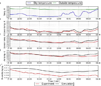
The outside and inside air conditions were quite stable over most winter nights except between 14 and 15 February 2010, when the greenhouse air temperature changed by about 4 K (Fig. 2.1a). This night was chosen for the validation process, as it was considered to be more suitable for studying the transient behaviour of the CFD model. The averages of the two air temperature and humidity sensors were compared with the CFD simulated greenhouse air temperature and humidity of the whole greenhouse volume. Additionally the average of the two roof temperature sensors was compared with the CFD simulated temperature of the whole greenhouse roof.
With regard to greenhouse air temperature, the difference between measured and simulated values was always less than 1 K (Fig. 2.1a). Both followed the same tendency after midnight, when there was a gradual drop in temperature until sunrise. The agreement of the transient temperature change was also good.
30 The time trend of the measured and CFD predicted humidity ratios are shown in Fig. 2.1c. The maximum difference between both values occurred after midnight, when the experimental values dropped more quickly than those predicted by the CFD model. This difference could be because the vapour source was considered as constant throughout the night for the CFD calculations, given the difficulty in detecting minor weight loses with the lysimeter. In all cases, the maximum difference was approximately 0.0007 kg kg-1, which is approximately 14% of the
[image:30.595.93.504.215.538.2]humidity ratio measured experimentally.
Fig. 2.1. Experimental and CFD simulated values of the greenhouse air temperature. Night 14 -15 February 2010: a) greenhouse air temperature, b) greenhouse roof temperature and c) greenhouse humidity ratio.
2.5.1.1
Assessment of model accuracy
31 The RMSE can be written as:
n
i
i Data i Mod y
y n 1
2 ,
, )
( 1
(2.3)
where n is the number of measurements (108 for this case), yMod,i is the simulated value at
period i and yData,i is the measured value. For the CFD model the RMSE values were:
inside temperature RMSE 0.367 oC cover temperature RMSE 0.89 oC relative humidity RMSE 6.5 % humidity ratio RMSE 0.00029 kg/kg
These values are in agreement with the RMSE values found by Baptista (2006), who developed a model for similar conditions and obtained an inside air temperature RMSE of 1.6 oC and relative humidity RMSE of 7%. As demonstrated by Baptista (2007), most greenhouse climate models have an RMSE of around 10%.
2.5.2
Steady state CFD simulations
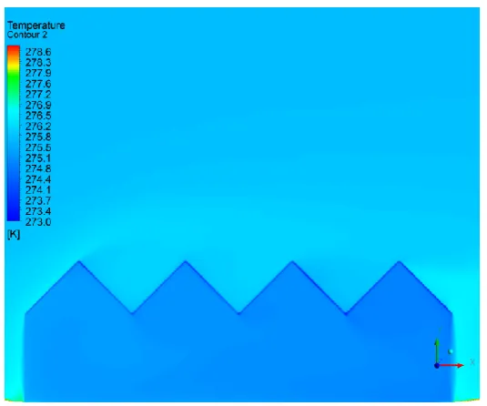
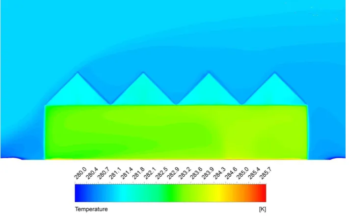
Figures 2.2 and 2.3 show the simulated greenhouse temperature and humidity at 3 AM during the night 14 to 15 February. At this time the soil heat flux was 9.8 W m-2, the outside air temperature was 275.7 K, the outside relative humidity was 71% and the wind speed was 2.3 m s-1. The equivalent sky temperature was calculated as 264.3 K, according to Berdahl, Martin and Sakkal (1983).
Figure 2.2 is a temperature map of a cross section of the simulated greenhouse under clear-sky night conditions, showing a minor thermal inversion; the greenhouse air was slightly cooler than the outside air since the average greenhouse air temperature was 275.0 K. The CFD model also gave the roof as the coolest surface of the greenhouse (approximately 1 K less than the greenhouse air), so this was the area with the highest tendency to produce condensation. Similar observations regarding thermal inversion and roof temperature in unheated greenhouses are widely supported by experimentation as well as simulation, since most of the heat losses are by infrared radiation emission (López Hernández, 2003).
32 Fig. 2.2. Map of temperature of a greenhouse cross section. Soil heat flux 9.8 W m-2, outside air 275.7 K, equivalent sky temperature 264.3 K. Wind speed 2.3 m s-1
33 Fig. 2.3. Map of humidity ratio of a greenhouse cross section. Soil heat flux 9.8 W m-2, outside air 275.7 K, equivalent sky temperature 264.3 K. Wind speed 2.3 m s-1. Air velocity vectors around the greenhouse are also shown.
The relationship between greenhouse humidity and roof temperature was investigated (Fig 2.4). Since sky temperature had a major effect on roof temperature, a number of simulations were run for a range of equivalent sky temperatures (263 K, 273 K and 276 K), covering clear to overcast conditions. Four soil heat fluxes were analysed (10, 25, 50 and 100 Wm-2), which covered from unheated to heated greenhouse conditions. This gave twelve combinations of boundary conditions for the simulations.
Figure 2.4a shows a strong correlation between roof temperature and greenhouse humidity ratio for the twelve simulations. The equation of the regression line was W = 0.34Tc+ 4.03 (R² =
0.99). For comparison, the experimental measurements of humidity ratio versus roof temperature are given in Fig. 2.4b. The experimental humidity regression line was W = 0.36Tc +
3.68 (R² = 0.97, n=105). In spite of the experimental measurements being taken under different conditions to those used in some of the CFD simulations (no greenhouse heating during the experiments), both CFD model and experimental data gave very good statistical indicators and the slope and constant coefficients of both regression lines were very similar. The greenhouse humidity was controlled by the roof temperature: due to the condensation on the roof it acted as the sink of air humidity, so that the greenhouse air reached a given value of water vapour content for each roof temperature.
34
2.5.3
Transient analysis of the night-time greenhouse climate
2.5.3.1
Condensation rate
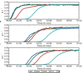
[image:34.595.148.440.257.512.2]The formation of condensation as a function of SHF and equivalent sky temperature was studied by running transient simulations with a time step of one minute. The initial humidity content of the greenhouse air was set to zero; from this point a constant source of water vapour was given to the greenhouse air.
Fig. 2.5. Condensation rate as a function of time for four soil heat fluxes (10, 25, 50 and 100 W m-2 and three equivalent sky temperatures a) 263 K, b) 273 K, c) 276 K.
Figure 2.5 shows that, independently of the SHF and sky temperature, the condensation curves had a similar pattern in which three phases can be differentiated:
a) Initial phase, where condensation has not yet begun.
b) Transitional phase (growing phase), where condensation rate increases sharply. (The slope of the condensation rate will be considered later.)
35 The main difference between Figs 2.5 a, b and c is the duration of the initial phase (zero condensation). The greater the SHF the later condensation starts. This can be explained by the fact that a higher SHF raises the greenhouse air and roof temperature, so condensation takes place at higher moisture content. The onset of condensation is also delayed for higher equivalent sky temperatures, due to the effect of the equivalent sky temperature on the cover temperature. The temperature of the cover is lower on clear nights since the net radiation loss from the greenhouse cover is greater.
Zero condensation phase. In this phase, cover temperature and air moisture content do not
fulfil the condensation conditions. This is the situation at the beginning of the night, when the cover temperature is higher than the dew point temperature of the greenhouse air.
The onset of condensation can be determined approximately by assuming uniform conditions in the greenhouse air. With this assumption, condensation will start when the greenhouse humidity reaches the humidity ratio at saturation.
The water vapour in the greenhouse air can be given by the mass balance equation as:
W
Sat
W
Init
V
G
air
T
rate
t
S
crop[Kg] ( 2.4) where WSat is humidity ratio at saturation, kg kg-1; WInit is initial humidity ratio of the
greenhouse air when transpiration started, kg kg-1; VG is greenhouse volume, m3; Trate is
transpiration rate, kg m-2 s-1; Scropis crop surface, m2; t is starting time of condensation, s; ρair
is air density, kg m-3.
If the cover temperature is known, the psychrometric properties of moist air such as
Wsat can be determined. For instance the ASAE Handbook, 2001 provides equations to
calculate humidity ratio from the dry-bulb temperature and relative humidity (ASAE Handbook, 2001) The cover temperature (Tc) can be accurately measured in the absence of
solar radiation. Where the crop transpiration rate and the initial water vapour content in the greenhouse air (WInit) are known, the time needed to reach the required water vapour in the
air can be calculated from Eq. 2.4.
Condensation transitional phase. This phase begins with the onset of condensation, and
36 x c be a x f 1 )
( with a and b >0 (2.5) A logistic curve has a stretched S-shape, initially modelling exponential growth and slowing down over time until the curve finally levels off. In the logistic function, a is defined as the limiting value (or asymptotic value) while b and c are parameters of the function.
When logistic functions are applied to the study of condensation, the parameter a is the steady-state condensation rate, which is the same as the constant vapour water source (in this case a = 0.247), the independent variable x is the time variable. The term b of Eq. 2.5 can be rewritten as
e , hence the term ecx becomes
t
e . For each case study, every condensation curve was statistically analysed against a logistic-type function, to find the coefficients which gave the best statistical results, using an R-language based software which used a variant of the Levenberg–Marquardt algorithm:
) 1 ( 247 . 0 ) ( (()/) t e t
f (2.6) where is the location parameter which translates the logistic function with time and
is the scale parameter which has the effect of stretching out the graph (Filiben, 2010). For all cases studied there was a strong correlation between simulation results and a logistic function. The minimum coefficient of determination (R2) was 0.97 for the 263_10 case.Attempts were made to develop a general curve that could fit all case studies under consideration. Since the starting time of condensation varied from one case to another (see Fig. 2.5), it was decided to take the origin (zero) as the time of onset of condensation for each individual curve. The condensation rate with time (Cr(t), g s-1) for the range of boundary
conditions analysed in this study can then be modelled by:
)) 06 . 19 / ) 89 . 65 (( 1 ( 247 . 0 ) ( t r e t C
[g s
-1] (2.7)
where time is expressed in minutes. The mean slope coefficient (
) was 19.06 and the mean absolute deviation was 2.8 for all condensation curves, and the mean coefficient was 65.89 and mean absolute deviation was 13Steady-state condensation rate phase. This is the final section of the condensation rate curve.
At steady state, the condensation rate equals the crop transpiration rate, which in this case and for the whole greenhouse crop was 0.247 g s-1.
37 Fig. 2.6. Logistic function for the condensation curve.
2.5.3.2
Time course of Relative Humidity
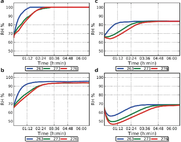
Relative humidity plays a major role on the development of relevant physiological processes such as transpiration and physiological disorders, as well as for the development of fungal diseases. As with the condensation rate, it was possible to plot the CFD predicted RH values against time for each pair of boundary conditions (SHF and equivalent sky temperature). An initial RH of 76% was used for simulations, the outside air RH at the beginning of the night between 14 and 15 February, which was the night chosen for the transient simulations (see Fig. 2.1).
38 In some cases, there was an initial reduction in RH, particularly for SHF = 100 W m-2. This was due to the transient simulation process, since for higher SHF values the increase in temperature was faster than the increase in absolute humidity.
Fig. 2.7. Time course of RH (%) with time (min) Top left: SHF 10 W m-2. Bottom left: soil heat flux 25 W m-2. Top right: soil heat flux 50 W m-2. Bottom right: soil heat flux 100 W m-2.
The simulations shown in Fig. 2.7 are for a constant source of water vapour, which is a model simplification due to the lack of knowledge on the night-time transpiration rate of greenhouse crops. The CFD model presented here allows for the implementation of a variable source of water vapour, since the model requires an updated input of variables such as outside temperature, humidity and wind speed, for each time step.
2.5.3.3
Model response to a step change in transpiration rate
39 reaction; in this case a change in the humidity source was chosen since humidity is a key issue in the condensation model.
The CFD simulation was made with the following boundary conditions: 273 K for the equivalent sky temperature and 100 W m-2 for the SHF. The wind speed, outside air temperature and humidity were the same as for the previous simulations (Table 2.2). Plant transpiration was considered as zero at the beginning of the simulation, and was then enabled to the previously used vapour source value of 0.247 g s-1 for the whole experimental greenhouse after 160 time steps (equivalent to 160 min) during which time the modelled air temperature and RH had reached steady-state (Fig. 2.8).
Fig. 2.8. Evolution of RH, condensation rate and temperature following a step-change in transpiration.
With the onset of transpiration, the RH began to increase, while the condensation rate began to increase once the water vapour in the air was sufficient to produce condensation on the roof (time ≈ 6:15). The reduction in the slope of the relative humidity curve also coincided with the onset of condensation, which indicated that the simulation is approaching to the steady state.
The final RH, 67.8%, was the same as the RH for the CFD simulation with plant transpiration enabled from the beginning. This confirms that RH depends on SHF under the set of outside air conditions considered in this study.
40 With regard to condensation, Fig. 2.8 shows the time course of the simulated condensation rate and the logistic function presented in Fig. 2.6. As mentioned previously, the logistic function was obtained for the water vapour source enabled from the start of the simulation. Both curves show a similar pattern, and their relative root mean square error was 10.39 %. As demonstrated by Baptista (2007) the performance of most available greenhouse climate models is around 10%.
Interestingly, condensation occurred for a relatively low greenhouse air RH (67.8%); condensation formed because the average roof temperature was 281.4 K, which was 6.4 K less than the average greenhouse air temperature. Under these conditions the average greenhouse air dew point temperature was slightly higher than the roof temperature. Moreover the greenhouse air near the roof was cooler than the average greenhouse air, so air conditions near the roof were more favourable to condensation formation.
2.6
Discussion
The CFD model predicted that the roof was the coolest surface of the greenhouse (approximately 1 K lower than the greenhouse air temperature for unheated greenhouses) since most of the energy losses were due to infrared radiation. This produced thermal inversion, which is a well known phenomenon in unheated Mediterranean greenhouses. The fact that the model is able to predict situations that occur in practice is a demonstration of its reliability. The model was also able to detect minor differences in temperature and humidity even for soil heat fluxes as low as 10 W m-2, as shown in Figs 2.2 and 2.3.
Since the roof was the coolest surface, its inner side was the sink of the water vapour produced by the crop, and the roof temperature controlled the humidity ratio in the greenhouse air. This strong link between roof temperature and water vapour content in the air was observed for heated and unheated greenhouses. This means that it may be possible to control greenhouse humidity and condensation by controlling roof temperature, although this in itself is quite difficult to achieve.
41 glass with IR reflective properties on the inner side being the warmest material. The study was conducted for an outside temperature of -10 °C in a heated greenhouse, so heat transfer by convection played a relevant role. In unheated greenhouses, where radiation losses are more important than convective losses, the far IR properties of the covering materials may have a major effect on condensation formation on the greenhouse roof and consequently on greenhouse absolute humidity. In contrast, RH is more dependent on SHF as mentioned before, and so it is less affected by the optical properties of the cover.
The aforementioned research was based on unventilated (closed) greenhouses. In CFD modelling it is difficult to consider infiltration loses, since this would require the definition of the location and geometry of the openings through which the greenhouse air could exit, information which is not usually available. In this research it was not possible to measure the infiltration rate, although infiltration would be expected to play a secondary role since most modern greenhouses can be considered as airtight. Nonetheless if an infiltration rate of 0.5 exchanges per hour is assumed, for the conditions shown in Figs. 2.2 & 2.3 (see section 2.3.2), the inside air humidity ratio Wint was 0.0039 kg kg-1 and the outside air humidity ratio Wout
was 0.00316 kg kg-1; the estimated rate of water vapour lost by infiltration was 0,0376 kg s-1, which is approximately 15% of the night time transpiration rate. This lost would have probably reduced the quantity of condensed water by about the same amount. Future model developments should try to improve accuracy by including a sink of water vapour due to infiltration.
The condensation model used a constant vapour source, i.e. constant transpiration from the crop. This is not a shortcoming of the model itself, since the transient model allows the inclusion of new boundary conditions for each time step. The model also reacted well to a step change in the water vapour source, a relevant variable, so changing boundary conditions can be included. The simulations were limited to a constant vapour source as there is a lack of knowledge on night-time crop transpiration and the link of transpiration rate with VPD and temperature at night. Probably the most reliable information on night transpiration in greenhouses comes from the work by Seginer, et al (1990). Values of transpiration presented in that work could be used in future simulations to analyse the greenhouse performance for different crops at different stages of development.
42 climates, for energy saving and to increase in crop production by CO2 enrichment, provided
that excessive humidity can be controlled (Stanghellini, Incrocci, Gázquez, & Dimauro, 2007). The CFD condensation model is currently being used to study the effect of a number of techniques such as the use of double walls, the night-time ventilation regime and selection of cover properties. In terms of night-time ventilation the model can answer questions such as: how much ventilation is needed for the control of humidity and temperature in heated and unheated greenhouses, what will happen if ventilators are open before the onset of condensation, or when is best to open the ventilators?
In terms of cover properties preliminary simulations have shown that, under clear sky conditions, a film with low emissivity, high reflectivity on the outer side and high emissivity, low reflectivity on the inner side can increase roof temperature by 1.9 K and greenhouse temperature by approximately 1.5 K. Such a temperature increase is relevant for unheated greenhouses and can be important in terms of energy saving for heated greenhouses.
The combination of these techniques under investigation is expected to provide relevant information for the development of strategies for humidity reduction.
2.7
Conclusions
A comprehensive analysis of the condensation process during night-time conditions was carried out. The ability of the CFD model to correctly predict the main greenhouse climate variables was validated against experimental data.
The simulations showed that there was a strong correlation between roof temperature and greenhouse humidity ratio for the twelve combinations of sky temperature and SHF considered in this study. In addition, it was found that the RH depended on the SHF more than on the roof temperature.
For a wide range of boundary conditions, greenhouse condensation followed the same characteristic pattern, so that the condensation rate could be modelled by a single logistic function that well represented all the conditions studied.
The ability of the model to correctly predict the greenhouse climate was tested through a step-change in the water vapour source value; the model reacted to this step-step-change and reached a final solution very similar to that achieved for a steady vapour source.
43 The condensation model applied in this study was developed by Bell (2003). This model was implemented as UDF into the general CFD simulation code. In Bell’s model the condensation rate is governed by the rate of diffusion of water vapour towards the cold surface.
According to Bird, Stewart and Lightfoot (1960), the species mass flux for water vapour at the liquid vapour interface (mH2O) can be written as
i O H i O H O H n W D v W m 2 2
2
[kg m-2 s-1] (A 2.1)
Where viis the interface normal velocity, D is the mass diffusivity and niis the interface
normal direction.
The mixture mass flux at the liquid vapour interface (m) is:
i O H
air m v
m
m
2
[kg m-2 s-1] (A 2.2) Since the liquid phase consist of only water
0
air
m (A 2.3) Substituting Eq. (A 2.1) into Eq. (A 2.2):
i O H O H n W D W v 2
2 1) (
1
[kg m-2 s-1] (A 2.4)
The CFD code treats the liquid-vapour interface as a wall with velocity v= 0. Therefore Eq. (A3) cannot be used directly for the calculation of condensation rate. However it is possible to include a mass sink/source term in the volume of the near wall cell to account for the condensation rate (where Acellwallis the cell area and
V
cell is the volume cell).cell wall cell V A v
m [kg m-3 s-1] (A 2.5) Substituting Eq. (A 2.3) into Eq. (A 2.4) .
cell wall cell i O H O H V A n W D W m 2
2 1) (
1
[kg m-3
s-1] (A 2.6)
44
m W mHO HO
2
2 [kg m
-3
s-1] (A 2.7) By writing Eqs. (A 2.5) and (A 2.6) into the source code of the UDF, the CFD code can calculate the volumetric mass source for the air mixture and the water vapour
Acknowledgments
The work presented here has been carried out within the project EUPHOROS. European Commission, Directorate General for Research, 7th Framework Programme of RTD, Theme 2 – Biotechnology, Agriculture & Food, contract 211457. This research has also been supported by INIA (project RTA2008-00109-C03) with contribution of FEDER founds. Thanks are also given to INIA fellowship FPI-INIA.
2.9
References
Ansys, F. (2009). User Guide 12.0. Lebanon, NH, USA.
ASHRAE Handbook (2001). Fundamentals. American Society of Heating, Refrigerating and Air Conditioning Engineers, Atlanta, GA, USA.
Baptista, F., Abreu, P., Meneses, J., & Bailey, B. (2001). Comparison of the climatic conditions and tomato crop productivity in Mediterranean greenhouses under two different natural ventilation management systems. Proc Int Symp AgriBuilding, 3-7.
Baptista, F. J. F. (2007). Modelling the climate in unheated tomato greenhouses and predicting Botrytis cinerea infection. Ph.D Thesis, Univerisade de Évora, Portugal.
Baxevanou, C., Bartzanas, T., Fidaros, D., & Kittas, C. (2008). Solar radiation distribution in a tunnel greenhouse. Acta Hort, 801, 855-862.
45 Berdahl, P., Martin, M., & Sakkal, F. (1983). Thermal performance of radiative cooling panels.
International Journal of Heat and Mass Transfer, 26(6), 871-880.
Bird, R. B., & Stewart, W. E. (1960). Lightfoot Transport Phenomena. John & Sons, New York, NY, USA.
Boulard, T., Fatnassi, H., Roy, J., Lagier, J., Fargues, J., Smits, N., et al. (2004). Effect of greenhouse ventilation on humidity of inside air and in leaf boundary-layer. Agricultural and Forest Meteorology, 125(3-4), 225-239.
Boulard, T., & Wang, S. (2000). Greenhouse crop transpiration simulation from external climate conditions. Agricultural and Forest Meteorology, 100(1), 25-34.
Bournet, P., Ould Khaoua, S., & Boulard, T. (2007). Numerical prediction of the effect of vent arrangements on the ventilation and energy transfer in a multi-span glasshouse using a bi-band radiation model. Biosystems Engineering, 98(2), 224-234.
Caird, M. A., Richards, J. H., & Donovan, L. A. (2007). Nighttime stomatal conductance and transpiration in C3 and C4 plants. Plant Physiology, 143(1), 4.
Campen, J., & Bot, G. (2001). SE--Structures and Environment:: Design of a Low-Energy Dehumidifying System for Greenhouses. Journal of Agricultural Engineering Research, 78(1), 65-73.
Campen, J., & Bot, G. (2002). SE--Structures and Environment:: Dehumidification in Greenhouses by Condensation on Finned Pipes. Biosystems Engineering, 82(2), 177-185. Campen, J., Bot, G., & De Zwart, H. (2003). Dehumidification of greenhouses at northern latitudes. Biosystems Engineering, 86(4), 487-493.