A WAVE MODEL OF A CIRCULAR TYRE
PACS REFERENCE:
R.J.Pinnington
I.S.V.R. University of Southampton Highfield
Southampton SO17 1BJ U.K.
tel+FAX: +30310 480645
E-mail rjpinnington@compuserve.com
ABSTRACT
The equations of motion of a curved tyre belt are derived for one-dimensional waves propagating around the belt and a standing wave across the belt. The effects of curvature, shear stiffness, rotary inertia, tension, rotational speed and air pressure are included. These are combined to give a sixth order wave equation, the solution of which gives three pairs of wave-number as a function of frequency. The application of the boundary conditions at the contact leads to the input and transfer mobilities for both in-plane and out of plane excitation. Observed are: low frequency rigid-body modes, belt bending modes and in-plane ring modes.
1.INTRODUCTION
When a rotating tyre interacts with the road surface, the time varying deformations are transmitted causing noise interior and exterior to the vehicle. To calculate this interaction with the road and also to determine the resulting vibration of the tyre surface it is first necessary to make a dynamic model of the tyre. The main exterior noise occurs between 500Hz and 3000Hz, a region where there is little modal behaviour of the belt flexural waves. An infinite flat belt wave model that included tension, transverse shear, rotary inertia and bending was made for this region [1]. However a full tyre model should embrace the whole low frequency range to include the vehicle interior noise between 50Hz and 500Hz, and the quasi-static slip of road-tyre interaction.
The objective here is therefore to extend the previous wave model to include: curvature, asymmetric belt and tyre rotation to the other parameters, and thus make a complete circular belt model. As the main effect of curvature is to couple transverse and longitudinal motion the response to both transverse and in-plane forces are obtained. The waves in the air cavity are neglected here, as they are only noticed at the first cavity resonance.
boundary conditions can be displacements, rotations, forces or moments. Presented here are only the frequency response functions for radial and circumferential forces.
2: EQUATIONS OF MOTION
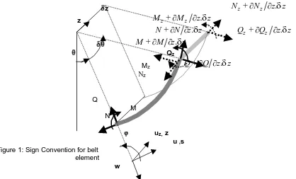
The tyre could be described as a curved, tensioned, Mindlin plate on distributed two-directional stiffness. Figure 1 shows a segment of length δs and width δz, in a tyre belt of radius a and width b, displaying the sign convention for positive directions, rotations, forces and moments. The belt is subjected to a net static pressure P which causes a static tension/length NS, NZ in the circumferencial and transverse directions s, z.. QS, QZ are the shear forces/length. N is the total static and dynamic circumferencial force/width. MS, MZ are the bending moments/length. The accompanying displacements are u,w, in the circumferential and radial directions. θ describes the geometric position and is related to the circumferential co-ordinate s as: s =aθ. The tyre rotates in the positive θ direction with angular velocity Ω.The belt is restrained either side by a side-wall of stiffnesses/ belt length of Ks , Kr , in the circumferential and radial directions.
In this section three groups of equations are presented: kinematic relationships, equilibrium of forces and moments, and the linking Hooke's Law relationships. It is also assumed that the averaged material properties of the cross-section are known, as reference will only be made to these single material values for the cross-section. The segment motion can be described by three variables; displacements u,w and the kinematic rotation Φ. For a Mindlin plate that can deform in both bending and shear, the slope at any position s in the s and z directions are respectively:
s s
,
z zw
w
s
β γ
z
β γ
∂
=
+
∂
=
+
∂
∂
(1a,b)
where βs ,βzand γs ,γz are the slopes due to bending and shear respectively. The kinematic
rotations Φs, ,Φz, in the s and z direction, of the element seen in Figure 1,including that due to the circumferential displacement u, are therefore:
δδz
N
z+ ∂
N
z∂
z z
.
δ
z
M
z+ ∂
M
z∂
z z
.
δ
N
+ ∂ ∂
N
z
.
δ
z
Q
z+ ∂
Q
z∂
z z
.
δ
δθδθ
M
+ ∂
M
∂
z
.
δ
z
θ θ Qz
Mz
Q
+ ∂ ∂
Q
z
.
δ
z
Νz
Q
M N
φφ uz, z
[image:2.596.103.521.307.560.2]u ,s
Figure 1: Sign Convention for belt element
s
,
zu
w
w
a
s
z
∂
∂
Φ = −
Φ = −
∂
∂
(2a,b)
The total angle
ϕ
in the s direction is the sum of the geometric rotationθ
and the kinematic rotationΦ
s.
The small change in slope over the lengthδ
s is therefore:
1
ss
a
s
δϕ
=
+
∂Φ
δ
∂
(3)
The circumferencial strain
ε
sand transverse strainε
zare:
s
,
z zu
u
w
s
a
z
ε
=
∂
+
ε
=
∂
∂
∂
(4a,b)
There are four equations of equilibrium: forces in the radial direction, forces in the circumferencial direction, and for moments in the s and z directions. The equilibrium of radial forces taken in line with the circumferencial shear force/width Qs. Substitution of the segment rotation in equation (2a) yields:
2
2 2
2
1
( , )
s z sz
Q
Q
w
P
P
a
p s z
N
N
w
w
s
z
a
s
z
a
µ
∂
∂
∂Φ
∂
µ
µ
+ Ω +
+
+
−
+
+
=
−
+ Ω
∂
∂
∂
∂
&&
(5)
where P is the net static pressure. p(s,z) is the dynamic pressure due to the side-wall and external radial force. Nz is the static transverse tensile force/length, N is the total static and dynamic circumferencial tensile force/width, Qz is the transverse shear force/width.
µ
is the belt mass/area. The last term is the extra centrifugal force due to displacement w.By resolving forces in the s direction in line with the circumferencial force/width N in Figure 2a, and substitution of the segment rotation in equation (2a), gives:
( )
2
1
,
s2
ss
K
N
c
s z
Q
u
w
u
s
a
s
a
b
τ
+
∂
+
+
∂Φ
=
µ
+
µ
+
∂
∂
&&
&
(6)
where Ks is the single side-wall circumferencial stiffness/belt length. The tangential external stress is
τ
.
. The second term from the left is the Coriolis force, which gives gyroscopic coupling between the axial and radial motion.The net moment, taken about the right hand end z axis of the segment is responsible only for the angular acceleration due to bending
β
&&
sas seen in equation 7a. A similar relation holds for the z direction:s s s s
,
z z z zM
M
Q
I
Q
I
s
β
z
β
∂
∂
−
=
−
=
∂
&&
∂
&&
(7a,b)
from the circumferential strain
ε
s:
1 2 2
sin
1
,
(1
)
,
2
s s
s s s s z
c c
l
Pl
N
N
A
N
Pa
a
N
b
φ
ε
µ
φ
φ
=
+
=
−
+ Ω
=
(8a,b,c)
where As is the belt axial stiffness/width. The static tensions Ns, Nz calculated in [2], are determined from the pressure, side-wall geometry and from resisting the centrifugal force
µΩ
2a.
2φ
cis the angle subtended by the side-wall,
φ
1is the angle the angle between side-wall
and the ground.
In the circumferencial and transverse directions the shear force/width Qs, Qz isrelated to the shear strain by the belt shear stiffness/width Ss,Sz.:
Q
s=
S
sγ
s,
Q
z=
S
zγ
z(9a,b)
The bending moment in the circumferencial and transverse directions can be written from [2] as equations 10. This concludes the component equations for the tyre belt.
2
,
s z
s s z z
w
M
B
M
B
s
a
z
β
β
∂
∂
= −
+
= −
∂
∂
(10a,b)
Equations 1-10 are reduced in [2] to a single sixth order wave equation. The solution selected here is a harmonic solution for a wave travelling in the positive s direction with m transverse half wavelengths, of the form wmexp(-ikms), umexp(-ikms). The sixth order wave equation is obtained
in the normalized wave-number zm=kma:
(
)
(
)(
)
(
)
(
(
)
)
(
)(
)
(
)(
)(
)
(
)
(
(
)
)
64 2 2 2
2 2 2
2
2 2
2 2 2
3 2
0
1
1
1
1
m s s
m L ce m s s s s c L s
s L m s L ce s s c s s
m
c s s m ce L
m ce L c s L s
s m c s m co
z
S
N
z
z
Pa
Z
K
N R
S
N
z
z
K
K
z
K
Pa
S
z
Z
N R
z
S
N
z
z
R
N
K
Pa
Z
z
K
Pa
Z
z
z
R
z
K
i
N
z
z
R
z
Z
=
+
−
+
+
−
−
+
+
+
+
−
−
+
−
−
−
+
+
−
+
+
+
−
−
+
+
+
+ +
−
−
−
−
−
±
+
−
−
(11)
The normalized cross section properties of shear stiffness, tension, pressure, rotational stiffness, sidewall and section modal stiffness, and centrifugal force are:
2
2 2 2
,
,
,
,
2
,
s s s rm zm
s s s m ce
s s s s s s
S
N
Pa
S
K
K
S
N
Pa
R
a
K
a
Z
a
A
A
A
B
A
A
µ
+
Ω
=
=
=
=
=
=
The two normalised non-dimensional wave-numbers zL, zc are for the longitudinal wave and the 'rotational wave' [1], which could also be called the first asymmetric Lamb wave [3]. The wave-numbers are defined by:
L2
( )
2s
z
a
A
µ
ω
=
,
2( )
2 sc s
I
z
a
B
ω
=
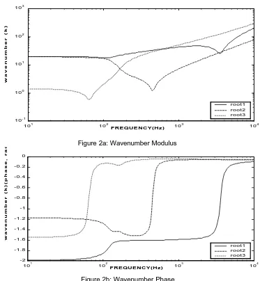
Figure 2a: Wavenumber Modulus
Figure 2b: Wavenumber Phase
The equation in zm2 is solved at each frequency to give three pairs of roots p=1,2,3 for each transverse mode group m. The normalised wave-numbers are of the form zpm i.e.
1m
,
2m,
3m,
z
z
z
±
±
±
for the anti-clockwise and clockwise wave. Here the three selectedwave-numbers kpm will take the sign and form of the wave that exists in the anticlockwise direction. The roots are complex in general and the true roots or waves are those that decay in the anti-clockwise direction and have the possibilities
(
± −
k
rik
i)
, where kr and ki are the real andimaginary wave-numbers. This wave can have three forms seen in Figures 2a,2b:
1. kr >> ki , a propagating or travelling wave with a small negative phase from the damping.
At 100Hz the root 3 wave cuts on and becomes a travelling bending-tension wave. 2. ki >> kr , the evanescent bending wave has a phase of -π/2 between 100Hz and 3kHz.
3.
k
r≈
k
i termed the 'complex wave', which always occurs in a pair± −
k
rik
i, e.g.root 2 and3 below 60Hz, form a rapidly decaying standing wave at the contact zone.
3: TRANSFER FUNCTIONS
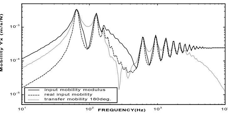
The transfer functions may now be found as each response is a sum of six waves, the amplitude of which is found from the six boundary conditions. These are continuity of displacement, continuity of the slope due to bending, and the input force and moment. For a stationary wheel, and the same material data as Figure 2, the input and transfer radial line mobility is given in Figure 3 and the tangential line mobility in Figure 4.
101 102 103 104
10- 1 100
101 102 103
wavenumber (k)
root1 root2 root3
FREQUENCY(Hz)
101 102 103 104
-2 -1.8 -1.6 -1.4 -1.2 -1 -0.8 -0.6 -0.4 -0.2 0
wavenumber (k)(phase, radians)
root1 root2 root3
Figure 3: Input and Transfer Mobility for radial line excitation
Figure 4: Input and Transfer Mobility for tangential line excitation
4: CONCLUSIONS
A tyre model for the whole working range from 0-3kHz has been made using a wave approach. This can provide transfer functions in the normal and tangential directions and can accommodate rotational effects such as centrifugal and Coriolis forces.
5:REFERENCES
1: R.J.Pinnington and A.R.Briscoe, A wave model for a pneumatic tyre belt. Submitted to Journal of Sound and Vibration.
2: R.J.Pinnington, A wave model for a circular pneumatic tyre, Submitted to Journal of Sound and Vibration.
6: ACKNOWLEGEMENT
This work was performed in the RATIN project under the E.C.Fifth Framework.
101 102 103 104
10- 5 10- 4 10- 3
Mobility Yy (m/s/N)
i n p u t m o b i l i t y m o d u l u s real input mobility transfer mobility 180deg.
FREQUENCY(Hz)
101 102 103 104
10- 5 10- 4 10- 3
Mobility Yx (m/s/N)
i n p u t m o b i l i t y m o d u l u s real input mobility transfer mobility 180deg.
[image:6.596.119.483.302.486.2]