Applied Intertemporal Optimization
Klaus Wälde
University of Mainz
CESifo, University of Bristol, Université catholique de Louvain
This book can freely be downloaded from www.waelde.com/aio. A print ver-sion can also be bought at this site.
@BOOK{Waelde11,
author = {Klaus Wälde}, year = 2011,
title = {Applied Intertemporal Optimization, Edition 1.1}, publisher = {Mainz University Gutenberg Press},
address = {Available atwww.waelde.com/aio} }
Gutenberg Press
Copyright (c) 2011 by Klaus Wälde www.waelde.com
Klaus Wälde Professor of Economics University of Mainz Jakob – Welder – Weg 4 55128 Mainz Germany Fax +49.6131.39-25588 Phone +49.6131.39-20143 [email protected] http://www.waelde.com/KTAP.html
Know Thyself _____________________________________
Academic Publishers
Please send or fax to
Know Thyself – Academic Publishers c/o Prof. Klaus Wälde
Jakob-Welder-Weg 4 55128 Mainz
Germany
Fax +49.6131.39-25588
Order form
(to be used by libraries and institutions only. Individuals can order online at www.waelde.com/aio)
Applied Intertemporal Optimization (Edition 1.2 plus)
_______ ____,___ EUR _________,___ EUR Quantity Price Total Amount
Name _________________ First Name ____________________
University/
Institution ______________________________________________________
Library ______________________________________________________
Address ______________________________________________________
Address ______________________________________________________
City _________________ ZIP code ____________________
Country _________________ State (if applicable) _____________
Phone Fax
Number _________________ Number ____________________
Email address _________________ @ _____________________________
Internet address ______________________________________________________
(Internet site at this address must display the email address from above. Email address will be used to confirm the order.)
1
Acknowledgments
This book is the result of many lectures given at various institutions, including the Bavarian Graduate Program in Economics, the Universities of Dortmund, Dresden, Frank-furt, Glasgow, Louvain-la-Neuve, Mainz, Munich and Würzburg and the European Com-mission in Brussels. I would therefore …rst like to thank the students for their questions and discussions. These conversations revealed the most important aspects in understand-ing model buildunderstand-ing and in formulatunderstand-ing maximization problems.
I also pro…ted from many discussions with economists and mathematicians from many other places. The high download …gures at repec.org show that the book is also widely used on an international level. I especially would like to thank Christian Bayer and Ken Sennewald for many insights into the more subtle issues of stochastic continuous time processes. I hope I succeeded in incorporating these insights into this book. I would also like to thank MacKichan for their repeated, quick and very useful support on typesetting issues in Scienti…c Word.
Overview
The basic structure of this book is simple to understand. It covers optimization methods and applications in discrete time and in continuous time, both in worlds with certainty and worlds with uncertainty.
discrete time continuous time deterministic setup Part I Part II
stochastic setup Part III Part IV
Table 0.0.1 Basic structure of this book
Solution methods
Parts and chapters Substitution Lagrange
Ch. 1 Introduction
Part I Deterministic models in discrete time
Ch. 2 Two-period models and di¤erence equations 2.2.1 2.3
Ch. 3 Multi-period models 3.8.2 3.1.2, 3.7
Part II Deterministic models in continuous time Ch. 4 Di¤erential equations
Ch. 5 Finite and in…nite horizon models 5.2.2, 5.6.1
Ch. 6 In…nite horizon models again
Part III Stochastic models in discrete time
Ch. 7 Stochastic di¤erence equations and moments
Ch. 8 Two-period models 8.1.4, 8.2
Ch. 9 Multi-period models 9.5 9.4
Part IV Stochastic models in continuous time Ch. 10 Stochastic di¤erential equations,
rules for di¤erentials and moments Ch. 11 In…nite horizon models
Ch. 12 Notation and variables, references and index
3
Each of these four parts is divided into chapters. As a quick reference, the table below provides an overview of where to …nd the four solution methods for maximization problems used in this book. They are the “substitution method”, “Lagrange approach”, “optimal control theory” and “dynamic programming”. Whenever we employ them, we refer to them as “Solving by”and then either “substitution”, “the Lagrangian”, “optimal control” or “dynamic programming”. As di¤erences and comparative advantages of methods can most easily be understood when applied to the same problem, this table also shows the most frequently used examples.
Be aware that these are not the only examples used in this book. Intertemporal pro…t maximization of …rms, capital asset pricing, natural volatility, matching models of the labour market, optimal R&D expenditure and many other applications can be found as well. For a more detailed overview, see the index at the end of this book.
Applications (selection)
optimal Dynamic Utility Central General Budget
control programming maximization planner equilibrium constraints
2.1,2.2 2.3.2 2.4 2.5.5 3.3 3.1,3.4, 3.8 3.2.3, 3.7 3.6
4.4.2 5 5.1,5.3, 5.6.1 5.6.3
6 6.1 6.4
8.1.4, 8.2 8.1 9.1, 9.2,9.3 9.1,9.4 9.2
10.3.2 11 11.1,11.3 11.5.1
Contents
1 Introduction 1
I
Deterministic models in discrete time
7
2 Two-period models and di¤erence equations 11
2.1 Intertemporal utility maximization . . . 11
2.1.1 The setup . . . 11
2.1.2 Solving by the Lagrangian . . . 13
2.2 Examples . . . 14
2.2.1 Optimal consumption. . . 14
2.2.2 Optimal consumption with prices . . . 16
2.2.3 Some useful de…nitions with applications . . . 17
2.3 The idea behind the Lagrangian . . . 21
2.3.1 Where the Lagrangian comes from I. . . 22
2.3.2 Shadow prices . . . 24
2.4 An overlapping generations model . . . 26
2.4.1 Technologies . . . 27
2.4.2 Households . . . 28
2.4.3 Goods market equilibrium and accumulation identity . . . 28
2.4.4 The reduced form . . . 29
2.4.5 Properties of the reduced form . . . 30
2.5 More on di¤erence equations . . . 32
2.5.1 Two useful proofs . . . 32
2.5.2 A simple di¤erence equation . . . 32
2.5.3 A slightly less but still simple di¤erence equation . . . 35
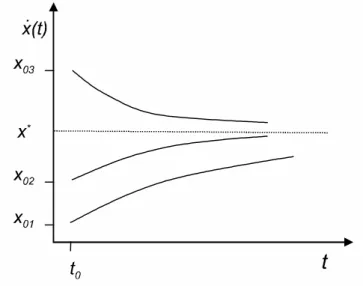
2.5.4 Fix points and stability. . . 36
2.5.5 An example: Deriving a budget constraint . . . 37
2.6 Further reading and exercises . . . 40
3 Multi-period models 45 3.1 Intertemporal utility maximization . . . 45
3.1.2 Solving by the Lagrangian . . . 46
3.2 The envelope theorem . . . 46
3.2.1 The theorem. . . 47
3.2.2 Illustration . . . 47
3.2.3 An example . . . 48
3.3 Solving by dynamic programming . . . 49
3.3.1 The setup . . . 49
3.3.2 Three dynamic programming steps . . . 50
3.4 Examples . . . 52
3.4.1 Intertemporal utility maximization with a CES utility function . . . 52
3.4.2 What is a state variable? . . . 55
3.4.3 Optimal R&D e¤ort . . . 57
3.5 On budget constraints . . . 59
3.5.1 From intertemporal to dynamic . . . 60
3.5.2 From dynamic to intertemporal . . . 60
3.5.3 Two versions of dynamic budget constraints . . . 62
3.6 A decentralized general equilibrium analysis . . . 62
3.6.1 Technologies . . . 62
3.6.2 Firms . . . 63
3.6.3 Households . . . 63
3.6.4 Aggregation and reduced form . . . 64
3.6.5 Steady state and transitional dynamics . . . 65
3.7 A central planner . . . 66
3.7.1 Optimal factor allocation . . . 66
3.7.2 Where the Lagrangian comes from II . . . 67
3.8 Growth of family size . . . 68
3.8.1 The setup . . . 68
3.8.2 Solving by substitution . . . 69
3.8.3 Solving by the Lagrangian . . . 69
3.9 Further reading and exercises . . . 70
II
Deterministic models in continuous time
75
4 Di¤erential equations 79 4.1 Some de…nitions and theorems . . . 794.1.1 De…nitions . . . 79
4.1.2 Two theorems . . . 80
4.2 Analyzing ODEs through phase diagrams . . . 81
4.2.1 One-dimensional systems . . . 81
4.2.2 Two-dimensional systems I - An example . . . 84
4.2.3 Two-dimensional systems II - The general case . . . 86
Contents 7
4.2.5 Multidimensional systems . . . 92
4.3 Linear di¤erential equations . . . 92
4.3.1 Rules on derivatives . . . 92
4.3.2 Forward and backward solutions of a linear di¤erential equation . . 94
4.3.3 Di¤erential equations as integral equations . . . 97
4.4 Examples . . . 97
4.4.1 Backward solution: A growth model . . . 97
4.4.2 Forward solution: Budget constraints . . . 98
4.4.3 Forward solution again: capital markets and utility . . . 100
4.5 Linear di¤erential equation systems . . . 102
4.6 Further reading and exercises . . . 102
5 Finite and in…nite horizon models 107 5.1 Intertemporal utility maximization - an introductory example . . . 107
5.1.1 The setup . . . 107
5.1.2 Solving by optimal control . . . 108
5.2 Deriving laws of motion . . . 109
5.2.1 The setup . . . 109
5.2.2 Solving by the Lagrangian . . . 109
5.2.3 Hamiltonians as a shortcut . . . 111
5.3 The in…nite horizon . . . 111
5.3.1 Solving by optimal control . . . 111
5.3.2 The boundedness condition . . . 113
5.4 Boundary conditions and su¢ cient conditions . . . 113
5.4.1 Free value of the state variable at the endpoint . . . 114
5.4.2 Fixed value of the state variable at the endpoint . . . 114
5.4.3 The transversality condition . . . 114
5.4.4 Su¢ cient conditions . . . 115
5.5 Illustrating boundary conditions . . . 116
5.5.1 A …rm with adjustment costs . . . 116
5.5.2 Free value at the end point. . . 119
5.5.3 Fixed value at the end point . . . 120
5.5.4 In…nite horizon and transversality condition . . . 120
5.6 Further examples . . . 121
5.6.1 In…nite horizon - optimal consumption paths . . . 121
5.6.2 Necessary conditions, solutions and state variables . . . 126
5.6.3 Optimal growth - the central planner and capital accumulation . . . 126
5.6.4 The matching approach to unemployment . . . 129
5.7 The present value Hamiltonian. . . 132
5.7.1 Problems without (or with implicit) discounting . . . 132
5.7.2 Deriving laws of motion . . . 133
5.8 Further reading and exercises . . . 136
6 In…nite horizon again 141 6.1 Intertemporal utility maximization . . . 141
6.1.1 The setup . . . 141
6.1.2 Solving by dynamic programming . . . 141
6.2 Comparing dynamic programming to Hamiltonians . . . 145
6.3 Dynamic programming with two state variables . . . 145
6.4 Nominal and real interest rates and in‡ation . . . 148
6.4.1 Firms, the central bank and the government . . . 148
6.4.2 Households . . . 149
6.4.3 Equilibrium . . . 149
6.5 Further reading and exercises . . . 152
6.6 Looking back . . . 155
III
Stochastic models in discrete time
157
7 Stochastic di¤erence equations and moments 161 7.1 Basics on random variables . . . 1617.1.1 Some concepts. . . 161
7.1.2 An illustration . . . 162
7.2 Examples for random variables . . . 162
7.2.1 Discrete random variables . . . 163
7.2.2 Continuous random variables . . . 163
7.2.3 Higher-dimensional random variables . . . 164
7.3 Expected values, variances, covariances and all that . . . 164
7.3.1 De…nitions . . . 164
7.3.2 Some properties of random variables . . . 165
7.3.3 Functions on random variables . . . 166
7.4 Examples of stochastic di¤erence equations . . . 168
7.4.1 A …rst example . . . 168
7.4.2 A more general case . . . 173
8 Two-period models 175 8.1 An overlapping generations model . . . 175
8.1.1 Technology . . . 175
8.1.2 Timing . . . 175
8.1.3 Firms . . . 176
8.1.4 Intertemporal utility maximization . . . 176
8.1.5 Aggregation and the reduced form for the CD case . . . 179
8.1.6 Some analytical results . . . 180
Contents 9
8.2 Risk-averse and risk-neutral households . . . 183
8.3 Pricing of contingent claims and assets . . . 187
8.3.1 The value of an asset . . . 187
8.3.2 The value of a contingent claim . . . 188
8.3.3 Risk-neutral valuation . . . 188
8.4 Natural volatility I . . . 189
8.4.1 The basic idea . . . 189
8.4.2 A simple stochastic model . . . 190
8.4.3 Equilibrium . . . 192
8.5 Further reading and exercises . . . 193
9 Multi-period models 197 9.1 Intertemporal utility maximization . . . 197
9.1.1 The setup with a general budget constraint . . . 197
9.1.2 Solving by dynamic programming . . . 198
9.1.3 The setup with a household budget constraint . . . 199
9.1.4 Solving by dynamic programming . . . 199
9.2 A central planner . . . 201
9.3 Asset pricing in a one-asset economy . . . 202
9.3.1 The model . . . 203
9.3.2 Optimal behaviour . . . 203
9.3.3 The pricing relationship . . . 204
9.3.4 More real results . . . 205
9.4 Endogenous labour supply . . . 207
9.5 Solving by substitution . . . 209
9.5.1 Intertemporal utility maximization . . . 209
9.5.2 Capital asset pricing . . . 210
9.5.3 Sticky prices . . . 212
9.5.4 Optimal employment with adjustment costs . . . 213
9.6 An explicit time path for a boundary condition . . . 215
9.7 Further reading and exercises . . . 216
IV
Stochastic models in continuous time
221
10 SDEs, di¤erentials and moments 225 10.1 Stochastic di¤erential equations (SDEs). . . 22510.1.1 Stochastic processes . . . 225
10.1.2 Stochastic di¤erential equations . . . 228
10.1.3 The integral representation of stochastic di¤erential equations . . . 232
10.2 Di¤erentials of stochastic processes . . . 232
10.2.1 Why all this? . . . 233
10.2.3 Computing di¤erentials for Poisson processes. . . 236
10.2.4 Brownian motion and a Poisson process. . . 238
10.3 Applications . . . 239
10.3.1 Option pricing. . . 239
10.3.2 Deriving a budget constraint . . . 240
10.4 Solving stochastic di¤erential equations . . . 242
10.4.1 Some examples for Brownian motion . . . 242
10.4.2 A general solution for Brownian motions . . . 245
10.4.3 Di¤erential equations with Poisson processes . . . 247
10.5 Expectation values . . . 249
10.5.1 The idea . . . 249
10.5.2 Simple results . . . 251
10.5.3 Martingales . . . 254
10.5.4 A more general approach to computing moments . . . 255
10.6 Further reading and exercises . . . 260
11 In…nite horizon models 267 11.1 Intertemporal utility maximization under Poisson uncertainty . . . 267
11.1.1 The setup . . . 267
11.1.2 Solving by dynamic programming . . . 269
11.1.3 The Keynes-Ramsey rule . . . 271
11.1.4 Optimal consumption and portfolio choice . . . 272
11.1.5 Other ways to determine ~c . . . 276
11.1.6 Expected growth . . . 277
11.2 Matching on the labour market: where value functions come from . . . 279
11.2.1 A household . . . 279
11.2.2 The Bellman equation and value functions . . . 280
11.3 Intertemporal utility maximization under Brownian motion . . . 281
11.3.1 The setup . . . 281
11.3.2 Solving by dynamic programming . . . 281
11.3.3 The Keynes-Ramsey rule . . . 283
11.4 Capital asset pricing . . . 283
11.4.1 The setup . . . 283
11.4.2 Optimal behaviour . . . 284
11.4.3 Capital asset pricing . . . 286
11.5 Natural volatility II . . . 287
11.5.1 An real business cycle model . . . 287
11.5.2 A natural volatility model . . . 290
11.5.3 A numerical approach . . . 291
11.6 Further reading and exercises . . . 292
Chapter 1
Introduction
This book provides a toolbox for solving dynamic maximization problems and for working with their solutions in economic models. Maximizing some objective function is central to Economics, it can be understood as one of the de…ning axioms of Economics. When it comes to dynamic maximization problems, they can be formulated in discrete or contin-uous time, under certainty or uncertainty. Various maximization methods will be used, ranging from the substitution method, via the Lagrangian and optimal control to dy-namic programming using the Bellman equation. Dydy-namic programming will be used for all environments, discrete, continuous, certain and uncertain, the Lagrangian for most of them. The substitution method is also very useful in discrete time setups. The optimal control theory, employing the Hamiltonian, is used only for deterministic continuous time setups. An overview was given in …g. 0.0.2 on the previous pages.
The general philosophy behind the style of this book says that what matters is an easy and fast derivation of results. This implies that a lot of emphasis will be put on examples and applications of methods. While the idea behind the general methods is sometimes illustrated, the focus is clearly on providing a solution method and examples of applications quickly and easily with as little formal background as possible. This is why the book is called applied intertemporal optimization.
Contents of parts I to IV
This book consists of four parts. In this …rst part of the book, we will get to know the simplest and therefore maybe the most useful structures to think about changes over time, to think about dynamics. Part I deals with discrete time models under certainty. The …rst chapter introduces the simplest possible intertemporal problem, a two-period problem. It is solved in a general way and for many functional forms. The methods used are the Lagrangian and simple substitution. Various concepts like the time preference rate and the intertemporal elasticities of substitution are introduced here as well, as they are widely used in the literature and are used frequently throughout this book. For those who want to understand the background of the Lagrangian, a chapter is included that shows the link between Lagrangians and solving by substitution. This will also give us the
opportunity to explain the concept of shadow prices as they play an important role e.g. when using Hamiltonians or dynamic programming. The two-period optimal consumption setup will then be put into a decentralized general equilibrium setup. This allows us to understand general equilibrium structures in general while, at the same time, we get to know the standard overlapping generations (OLG) general equilibrium model. This is one of the most widely used dynamic models in Economics. Chapter 2 concludes by reviewing some aspects of di¤erence equations.
Chapter 3 then covers in…nite horizon models. We solve a typical maximization prob-lem …rst by using the Lagrangian again and then by dynamic programming. As dynamic programming regularly uses the envelope theorem, this theorem is …rst reviewed in a sim-ple static setup. Examsim-ples for in…nite horizon problems, a general equilibrium analysis of a decentralized economy, a typical central planner problem and an analysis of how to treat family or population growth in optimization problems then complete this chapter. To complete the range of maximization methods used in this book, the presentation of these examples will also use the method of “solving by inserting”.
Part II covers continuous time models under certainty. Chapter 4 …rst looks at dif-ferential equations as they are the basis of the description and solution of maximization problems in continuous time. First, some useful de…nitions and theorems are provided. Second, di¤erential equations and di¤erential equation systems are analyzed qualitatively by the so-called “phase-diagram analysis”. This simple method is extremely useful for understanding di¤erential equations per se and also for later purposes for understand-ing qualitative properties of solutions to maximization problems and properties of whole economies. Linear di¤erential equations and their economic applications are then …nally analyzed before some words are spent on linear di¤erential equation systems.
Chapter 5 presents a new method for solving maximization problems - the Hamil-tonian. As we are now in continuous time, two-period models do not exist. A distinction will be drawn, however, between …nite and in…nite horizon models. In practice, this dis-tinction is not very important as, as we will see, optimality conditions are very similar for …nite and in…nite maximization problems. After an introductory example on maximiza-tion in continuous time by using the Hamiltonian, the simple link between Hamiltonians and the Lagrangian is shown.
The solution to maximization problems in continuous time will consist of one or several di¤erential equations. As a unique solution to di¤erential equations requires boundary conditions, we will show how boundary conditions are related to the type of maximization problem analyzed. The boundary conditions di¤er signi…cantly between …nite and in…nite horizon models. For the …nite horizon models, there are initial or terminal conditions. For the in…nite horizon models, we will get to know the transversality condition and other related conditions like the No-Ponzi-game condition. Many examples and a comparison between the present-value and the current-value Hamiltonian conclude this chapter.
3
of dynamic programming in continuous time, e.g. the structure of the Bellman equation, can already be treated here under certainty. This chapter will also provide a comparison between the Hamiltonian and dynamic programming and look at a maximization problem with two state variables. An example from monetary economics on real and nominal interest rates concludes the chapter.
In part III, the world becomes stochastic. Parts I and II provided many optimization methods for deterministic setups, both in discrete and continuous time. All economic questions that were analyzed were viewed as “su¢ ciently deterministic”. If there was any uncertainty in the setup of the problem, we simply ignored it or argued that it is of no importance for understanding the basic properties and relationships of the economic question. This is a good approach to many economic questions.
Generally speaking, however, real life has few certain components. Death is certain, but when? Taxes are certain, but how high are they? We know that we all exist - but don’t ask philosophers. Part III (and part IV later) will take uncertainty in life seriously and incorporate it explicitly in the analysis of economic problems. We follow the same distinction as in part I and II - we …rst analyse the e¤ects of uncertainty on economic behaviour in discrete time setups in part III and then move to continuous time setups in part IV.
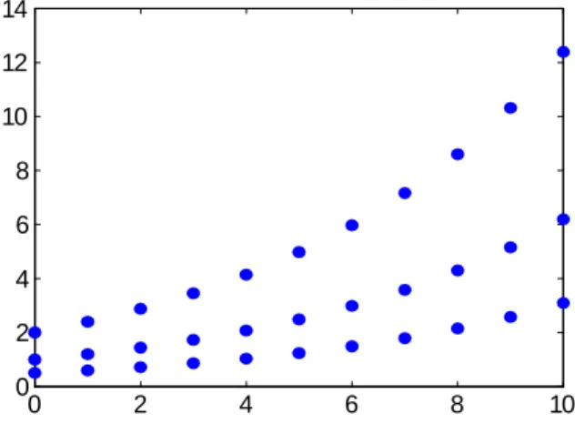
Chapter 7 and 8 are an extended version of chapter 2. As we are in a stochastic world, however, chapter 7 will …rst spend some time reviewing some basics of random variables, their moments and distributions. Chapter 7 also looks at di¤erence equations. As they are now stochastic, they allow us to understand how distributions change over time and how a distribution converges - in the example we look at - to a limiting distribution. The limiting distribution is the stochastic equivalent to a …x point or steady state in deterministic setups.
Chapter 8 looks at maximization problems in this stochastic framework and focuses on the simplest case of two-period models. A general equilibrium analysis with an overlapping generations setup will allow us to look at the new aspects introduced by uncertainty for an intertemporal consumption and saving problem. We will also see how one can easily understand dynamic behaviour of various variables and derive properties of long-run distributions in general equilibrium by graphical analysis. One can for example easily obtain the range of the long-run distribution for capital, output and consumption. This increases intuitive understanding of the processes at hand tremendously and helps a lot as a guide to numerical analysis. Further examples include borrowing and lending between risk-averse and risk-neutral households, the pricing of assets in a stochastic world and a …rst look at ’natural volatility’, a view of business cycles which stresses the link between jointly endogenously determined short-run ‡uctuations and long-run growth.
matching model of unemployment. The next section then covers how many maximization problems can be solved without using dynamic programming or the Lagrangian. In fact, many problems can be solved simply by inserting, despite uncertainty. This will be illustrated with many further applications. A …nal section on …nite horizons concludes.
Part IV is the …nal part of this book and, logically, analyzes continuous time models under uncertainty. The choice between working in discrete or continuous time is partly driven by previous choices: If the literature is mainly in discrete time, students will …nd it helpful to work in discrete time as well. The use of discrete time methods seem to hold for macroeconomics, at least when it comes to the analysis of business cycles. On the other hand, when we talk about economic growth, labour market analyses and …nance, continuous time methods are very prominent.
Whatever the tradition in the literature, continuous time models have the huge ad-vantage that they are analytically generally more tractable, once some initial investment into new methods has been digested. As an example, some papers in the literature have shown that continuous time models with uncertainty can be analyzed in simple phase diagrams as in deterministic continuous time setups. See ch. 10.6and ch. 11.6 on further reading for references from many …elds.
To facilitate access to the magical world of continuous time uncertainty, part IV presents the tools required to work with uncertainty in continuous time models. It is probably the most innovative part of this book as many results from recent research ‡ow directly into it. This part also most strongly incorporates the central philosophy behind writing this book: There will be hardly any discussion of formal mathematical aspects like probability spaces, measurability and the like. While some will argue that one can not work with continuous time uncertainty without having studied mathematics, this chapter and the many applications in the literature prove the opposite. The objective here is to clearly make the tools for continuous time uncertainty available in a language that is ac-cessible for anyone with an interest in these tools and some “feeling”for dynamic models and random variables. The chapters on further reading will provide links to the more mathematical literature. Maybe this is also a good point for the author of this book to thank all the mathematicians who helped him gain access to this magical world. I hope they will forgive me for “betraying their secrets”to those who, maybe in their view, were not appropriately initiated.
Chapter 10 provides the background for optimization problems. As in part II where we …rst looked at di¤erential equations before working with Hamiltonians, here we will …rst look at stochastic di¤erential equations. After some basics, the most interesting aspect of working with uncertainty in continuous time follows: Ito’s lemma and, more generally, change-of-variable formulas for computing di¤erentials will be presented. As an application of Ito’s lemma, we will get to know one of the most famous results in Economics - the Black-Scholes formula. This chapter also presents methods for how to solve stochastic di¤erential equations or how to verify solutions and compute moments of random variables described by a stochastic process.
5
the classic intertemporal utility maximization problem both for Poisson uncertainty and for Brownian motion. The chapter also shows the link between Poisson processes and matching models of the labour market. This is very useful for working with extensions of the simple matching model that allows for savings. Capital asset pricing and natural volatility conclude the chapter.
From simple to complex setups
Given that certain maximization problems are solved many times - e.g. utility max-imization of a household …rst under certainty in discrete and continuous time and then under uncertainty in discrete and continuous time - and using many methods, the “steps how to compute solutions” can be easily understood: First, the discrete deterministic two-period approach provides the basic intuition or feeling for a solution. Next, in…nite horizon problems add one dimension of complexity by “taking away” the simple bound-ary condition of …nite horizon models. In a third step, uncertainty adds expectations operators and so on. By gradually working through increasing steps of sophistication and by linking back to simple but structurally identical examples, intuition for the complex setups is built up as much as possible. This approach then allows us to …nally understand the beauty of e.g. Keynes-Ramsey rules in continuous time under Poisson uncertainty or Brownian motion.
Even more motivation for this book
Why teach a course based on this book? Is it not boring to go through all these methods? In a way, the answer is yes. We all want to understand certain empirical regularities or understand potential fundamental relationships and make exciting new empirically testable predictions. In doing so, we also all need to understand existing work and eventually present our own ideas. It is probably much more boring to be hindered in understanding existing work and be almost certainly excluded from presenting our own ideas if we always spend a long time trying to understand how certain results were derived. How did this author get from equation (1) and (2) to equation (3)? The major advantage of economic analysis over other social sciences is its strong foundation in formal models. These models allow us to discuss questions much more precisely as expressions like “marginal utility”, “time preference rate” or “Keynes-Ramsey rule” reveal a lot of information in a very short time. It is therefore extremely useful to …rst spend some time in getting to know these methods and then to try to do what Economics is really about: understand the real world.
The audience for this book
Before this book came out, it had been tested for at least ten years in many courses. There are two typical courses which were based on this book. A third year Bachelor course (for ambitious students) can be based on parts I and II, i.e. on maximization and applications in discrete and continuous time under certainty. Such a course typically took 14 lectures of 90 minutes each plus the same number of tutorials. It is also possible to present the material also in 14 lectures of 90 minutes each plus only 7 tutorials. Presenting the material without tutorials requires a lot of energy from the students to go through the problem sets on their own. One can, however, discuss some selected problem sets during lectures.
The other typical course which was based on this book is a …rst-year PhD course. It would review a few chapters of part I and part II (especially the chapters on dynamic programming) and cover in full the stochastic material of part III and part IV. It also requires fourteen 90 minute sessions and exercise classes help even more, given the more complex material. But the same type of arrangements as discussed for the Bachelor course did work as well.
Of course, any other combination is feasible. From my own experience, teaching part I and II in a third year Bachelor course allows teaching of part III and IV at the Master level. Of course, Master courses can be based on any parts of this book, …rst-year PhD courses can start with part I and II and second-year …eld courses can use material of part III or IV. This all depends on the ambition of the programme, the intention of the lecturer and the needs of the students.
Part I
Deterministic models in discrete
time
9
This book consists of four parts. In this …rst part of the book, we will get to know the simplest and therefore maybe the most useful structures to think about changes over time, to think about dynamics. Part I deals with discrete time models under certainty. The …rst chapter introduces the simplest possible intertemporal problem, a two-period problem. It is solved in a general way and for many functional forms. The methods used are the Lagrangian and simple substitution. Various concepts like the time preference rate and the intertemporal elasticities of substitution are introduced here as well, as they are widely used in the literature and are used frequently throughout this book. For those who want to understand the background of the Lagrangian, a chapter is included that shows the link between Lagrangians and solving by substitution. This will also give us the opportunity to explain the concept of shadow prices as they play an important role e.g. when using Hamiltonians or dynamic programming. The two-period optimal consumption setup will then be put into a decentralized general equilibrium setup. This allows us to understand general equilibrium structures in general while, at the same time, we get to know the standard overlapping generations (OLG) general equilibrium model. This is one of the most widely used dynamic models in Economics. Chapter 2 concludes by reviewing some aspects of di¤erence equations.
Chapter 2
Two-period models and di¤erence
equations
Given that the idea of this book is to start from simple structures and extend them to the more complex ones, this chapter starts with the simplest intertemporal problem, a two-period decision framework. This simple setup already allows us to illustrate the basic dynamic trade-o¤s. Aggregating over individual behaviour, assuming an overlapping-generations (OLG) structure, and putting individuals in general equilibrium provides an understanding of the issues involved in these steps and in identical steps in more general settings. Some revision of properties of di¤erence equations concludes this chapter.
2.1
Intertemporal utility maximization
2.1.1
The setup
Let there be an individual living for two periods, in the …rst she is young, in the second she is old. Let her utility function be given by
Ut =U cyt; cot+1 U(ct; ct+1); (2.1.1)
where consumption when young and old are denoted by cyt andcot+1 orct andct+1;
respec-tively, when no ambiguity arises. The individual earns labour incomewt in both periods.
It could also be assumed that she earns labour income only in the …rst period (e.g. when retiring in the second) or only in the second period (e.g. when going to school in the …rst). Here, with st denoting savings, her budget constraint in the …rst period is
ct+st =wt (2.1.2)
and in the second it reads
ct+1 =wt+1+ (1 +rt+1)st: (2.1.3)
Interest paid on savings in the second period are given byrt+1:All quantities are expressed
in units of the consumption good (i.e. the price of the consumption good is set equal to one. See ch. 2.2.2 for an extension where the price of the consumption good is pt:).
This budget constraint says something about the assumptions made on the timing of wage payments and savings. What an individual can spend in period two is principal and interest on her savingsstof the …rst period. There are no interest payments in period one.
This means that wages are paid and consumption takes place at the end of period 1 and savings are used for some productive purposes (e.g. …rms use it in the form of capital for production) in period 2. Therefore, returns rt+1 are determined by economic conditions
in period 2 and have the index t+ 1: Timing is illustrated in the following …gure.
st =wt ct
wt ct
t
(1 +rt+1)st
ct+1 wt+1
t+ 1
Figure 2.1.1 Timing in two-period models
These two budget constraints can be merged into one intertemporal budget constraint by substituting out savings,
wt+ (1 +rt+1) 1
wt+1 =ct+ (1 +rt+1) 1
ct+1: (2.1.4)
It should be noted that by not restricting savings to be non-negative in (2.1.2) or by equat-ing the present value of income on the left-hand side with the present value of consumption on the right-hand side in (2.1.4), we assume perfect capital markets: individuals can save and borrow any amount they desire. Equation (2.2.14) provides a condition under which individuals save.
Adding the behavioural assumption that individuals maximize utility, the economic behaviour of an individual is described completely and one can derive her consumption and saving decisions. The problem can be solved by a Lagrange approach or simply by substitution. The latter will be done in ch. 2.2.1 and 3.8.2 in deterministic setups or extensively in ch. 8.1.4 for a stochastic framework. Substitution transforms an optimiza-tion problem with a constraint into an unconstrained problem. We will use a Lagrange approach now.
The maximization problem readsmaxct; ct+1(2.1.1) subject to the intertemporal budget constraint (2.1.4). The household’s control variables are ct and ct+1: As they need to be
2.1. Intertemporal utility maximization 13
of each other. Wages and interest rates are exogenously given to the household. When choosing consumption levels, the reaction of these quantities to the decision of our house-hold is assumed to be zero - simply because the househouse-hold is too small to have an e¤ect on economy-wide variables.
2.1.2
Solving by the Lagrangian
We will solve this maximization problem by using the Lagrange function. This function will now be presented simply and its structure will be explained in a “recipe sense”, which is the most useful one for those interested in quick applications. For those interested in more background, ch. 2.3 will show the formal principles behind the Lagrangian. The Lagrangian for our problem reads
L =U(ct; ct+1) + wt+ (1 +rt+1) 1wt+1 ct (1 +rt+1) 1ct+1 , (2.1.5)
where is a parameter called the Lagrange multiplier. The Lagrangian always consists of two parts. The …rst part is the objective function, the second part is the product of the Lagrange multiplier and the constraint, expressed as the di¤erence between the right-hand side and the left-hand side of (2.1.4). Technically speaking, it makes no di¤erence whether one subtracts the left-hand side from the hand side as here or vice versa - right-hand side minus left-right-hand side. Reversing the di¤erence would simply change the sign of the Lagrange multiplier but not change the …nal optimality conditions. Economically, however, one would usually want a positive sign of the multiplier, as we will see in ch.2.3.
The …rst-order conditions are
Lct =Uct(ct; ct+1) = 0;
Lct+1 =Uct+1(ct; ct+1) [1 +rt+1]
1
= 0;
L =wt+ (1 +rt+1) 1
wt+1 ct (1 +rt+1) 1
ct+1 = 0:
Clearly, the last …rst-order condition is identical to the budget constraint. Note that there are three variables to be determined, consumption for both periods and the Lagrange multiplier . Having at least three conditions is a necessary, though not su¢ cient (they might, generally speaking, be linearly dependent) condition for this to be possible.
The …rst two …rst-order conditions can be combined to give
Uct(ct; ct+1) = (1 +rt+1)Uct+1(ct; ct+1) = : (2.1.6)
Marginal utility from consumption today on the left-hand side must equal marginal utility tomorrow, corrected by the interest rate, on the right-hand side. The economic meaning of this correction can best be understood when looking at a version with nominal budget constraints (see ch. 2.2.2).
today to consumption ct+1 tomorrow. This equation together with the budget constraint
(2.1.4) provides a two-dimensional system: two equations in two unknowns, ct and ct+1.
These equations therefore allow us in principle to compute these endogenous variables as a function of exogenously given wages and interest rates. This would then be the solution to our maximization problem. The next section provides an example where this is indeed the case.
2.2
Examples
2.2.1
Optimal consumption
The setup
This …rst example allows us to solve explicitly for consumption levels in both periods. Let preferences of households be represented by
Ut= lnct+ (1 ) lnct+1: (2.2.1)
This utility function is often referred to as Cobb-Douglas or logarithmic utility function. Utility from consumption in each period, instantaneous utility, is given by the logarithm of consumption. Instantaneous utility is sometimes also referred to as felicity function. As lnc has a positive …rst and negative second derivative, higher consumption increases instantaneous utility but at a decreasing rate. Marginal utility from consumption is decreasing in (2.2.1). The parameter captures the importance of instantaneous utility in the …rst relative to instantaneous utility in the second. Overall utilityUt is maximized
subject to the constraint we know from (2.1.4) above,
Wt =ct+ (1 +rt+1) 1ct+1; (2.2.2)
where we denote the present value of labour income by
Wt wt+ (1 +rt+1) 1
wt+1: (2.2.3)
Again, the consumption good is chosen as numeraire good and its price equals unity. Wages are therefore expressed in units of the consumption good.
Solving by the Lagrangian
The Lagrangian for this problem reads
L = lnct+ (1 ) lnct+1+ Wt ct (1 +rt+1) 1ct+1 :
The …rst-order conditions are
Lct = (ct)
1
= 0;
Lct+1 = (1 ) (ct+1)
1
[1 +rt+1] 1
= 0;
2.2. Examples 15
The solution
Dividing …rst-order conditions gives 1 ct+1
ct = 1 +rt+1 and therefore
ct =
1 (1 +rt+1)
1 ct+1:
This equation corresponds to our optimality rule (2.1.6) derived above for the more general case. Inserting into the budget constraint (2.2.2) yields
Wt=
1 + 1 (1 +rt+1)
1
ct+1 =
1
1 (1 +rt+1)
1 ct+1
which is equivalent to
ct+1 = (1 ) (1 +rt+1)Wt: (2.2.4)
It follows that
ct = Wt: (2.2.5)
Apparently, optimal consumption decisions imply that consumption when young is given by a share of the present value Wt of life-time income at time t of the individual
under consideration. Consumption when old is given by the remaining share 1 plus interest payments, ct+1 = (1 +rt+1) (1 )Wt: Equations (2.2.4) and (2.2.5) are the
solution to our maximization problem. These expressions are sometimes called “closed-form”solutions. A (closed-form) solution expresses the endogenous variable, consumption in our case, as a function only of exogenous variables. Closed-form solution is a di¤erent word for closed-loop solution. For further discussion see ch. 5.6.2.
Assuming preferences as in (2.2.1) makes modelling sometimes easier than with more complex utility functions. A drawback here is that the share of lifetime income consumed in the …rst period and therefore the savings decision is independent of the interest rate, which appears implausible. A way out is given by the CES utility function (see below at (2.2.10)) which also allows for closed-form solutions for consumption (for an example in a stochastic setup, see exercise6in ch.8.1.4). More generally speaking, such a simpli…cation should be justi…ed if some aspect of an economy that is fairly independent of savings is the focus of some analysis.
Solving by substitution
Let us now consider this example and see how this maximization problem could have been solved without using the Lagrangian. The principle is simply to transform an op-timization problem with constraints into an opop-timization problem without constraints. This is most simply done in our example by replacing the consumption levels in the ob-jective function (2.2.1) by the consumption levels from the constraints (2.1.2) and (2.1.3). The unconstrained maximization problem then reads maxUt by choosing st;where
This objective function shows the trade-o¤ faced by anyone who wants to save nicely. High savings reduce consumption today but increase consumption tomorrow.
The …rst-order condition, i.e. the derivative with respect to savingst; is simply
wt st
= (1 +rt+1)
1
wt+1+ (1 +rt+1)st
:
When this is solved for savings st; we obtain
wt+1
1 +rt+1
+st = (wt st)
1
, wt+1 1 +rt+1
=wt
1
st
1 ,
st = (1 )wt
wt+1
1 +rt+1
=wt Wt;
whereWtis life-time income as de…ned after (2.2.2). To see that this is consistent with the
solution by Lagrangian, compute …rst-period consumption and …nd ct=wt st= Wt
-which is the solution in (2.2.5).
What have we learned from using this substitution method? We see that we do not need “sophisticated”tools like the Lagrangian as we can solve a “normal”unconstrained problem - the type of problem we might be more familiar with from static maximization setups. But the steps to obtain the …nal solution appear somewhat more “curvy”and less elegant. It therefore appears worthwhile to become more familiar with the Lagrangian.
2.2.2
Optimal consumption with prices
Consider now again the utility function (2.1.1) and maximize it subject to the constraints
ptct +st = wt and pt+1ct+1 = wt+1 + (1 +rt+1)st: The di¤erence to the introductory
example in ch.2.1consists in the introduction of an explicit price pt for the consumption
good. The …rst-period budget constraint now equates nominal expenditure for consump-tion (ptct is measured in, say, Euro, Dollar or Yen) plus nominal savings to nominal wage
income. The second period constraint equally equates nominal quantities. What does an optimal consumption rule as in (2.1.6) now look like?
The Lagrangian is, now using an intertemporal budget constraint with prices,
L=U(ct; ct+1) + Wt ptct (1 +rt+1) 1pt+1ct+1 :
The …rst-order conditions for ct and ct+1 are
Lct =Uct(ct; ct+1) pt = 0;
Lct+1 =Uct+1(ct; ct+1) (1 +rt+1)
1
pt+1 = 0
and the intertemporal budget constraint. Combining them gives
Uct(ct; ct+1)
pt
= Uct+1(ct; ct+1)
pt+1[1 +rt+1]
1 ,
Uct(ct; ct+1)
Uct+1(ct; ct+1)
= pt
pt+1[1 +rt+1]
2.2. Examples 17
This equation says that marginal utility of consumption today relative to marginal utility of consumption tomorrow equals the relative price of consumption today and tomorrow. This optimality rule is identical for a static 2-good decision problem where optimality requires that the ratio of marginal utilities equals the relative price. The relative price here is expressed in a present value sense as we compare marginal utilities at two points in time. The price pt is therefore divided by the price tomorrow, discounted by the next
period’s interest rate, pt+1[1 +rt+1] 1:
In contrast to what sometimes seems common practice, we will not call (2.2.6) a solution to the maximization problem. This expression (frequently referred to as the Euler equation) is simply an expression resulting from …rst-order conditions. Strictly speaking, (2.2.6) is only a necessary condition for optimal behaviour - and not more. As de…ned above, a solution to a maximization problem is a closed-form expression as for example in (2.2.4) and (2.2.5). It gives information on levels - and not just on changes as in (2.2.6). Being aware of this important di¤erence, in what follows, the term “solving a maximization problem”will nevertheless cover both analyses. Those which stop at the Euler equation and those which go all the way towards obtaining a closed-form solution.
2.2.3
Some useful de…nitions with applications
In order to be able to discuss results in subsequent sections easily, we review some de…ni-tions here that will be used frequently in later parts of this book. We are mainly interested in the intertemporal elasticity of substitution and the time preference rate. While a lot of this material can be found in micro textbooks, the notation used in these books di¤ers of course from the one used here. As this book is also intended to be as self-contained as possible, this short review can serve as a reference for subsequent explanations. We start with the
Marginal rate of substitution (MRS)
Let there be a consumption bundle(c1; c2; ::::; cn):Let utility be given byu(c1; c2; ::::; cn)
which we abbreviate to u(:):The MRS between good i and good j is then de…ned by
M RSij(:)
@u(:)=@ci
@u(:)=@cj
: (2.2.7)
It gives the increase of consumption of good j that is required to keep the utility level at u(c1; c2; ::::; cn) when the amount of i is decreased marginally. By this de…nition, this
amount is positive if both goods are normal goods - i.e. if both partial derivatives in (2.2.7) are positive. Note that de…nitions used in the literature can di¤er from this one. Some replace ’decreased’by ’increased’(or - which has the same e¤ect - replace ’increase’ by ’decrease’) and thereby obtain a di¤erent sign.
Why this is so can easily be shown: Consider the total di¤erential of u(c1; c2; ::::; cn);
keeping all consumption levels apart from ci and cj …x. This yields
du(c1; c2; ::::; cn) =
@u(:)
@ci
dci+
@u(:)
@cj
The overall utility level u(c1; c2; ::::; cn) does not change if
du(:) = 0, dcj
dci
= @u(:)
@ci
=@u(:) @cj
M RSij(:):
Equivalent terms
As a reminder, the equivalent term to the MRS in production theory is the mar-ginal rate of technical substitution M RT Sij(:) = @f@f((::))=@x=@xij where the utility function was
replaced by a production function and consumption ck was replaced by factor inputs xk.
On a more economy-wide level, there is the marginal rate of transformationM RTij(:) = @G(:)=@yi
@G(:)=@yj where the utility function has now been replaced by a transformation functionG
(maybe better known as production possibility curve) and the yk are output of good k.
The marginal rate of transformation gives the increase in output of good j when output of good i is marginally decreased.
(Intertemporal) elasticity of substitution
Though our main interest is a measure ofintertemporal substitutability, we …rst de…ne the elasticity of substitution in general. As with the marginal rate of substitution, the de…nition implies a certain sign of the elasticity. In order to obtain a positive sign (with normal goods), we de…ne the elasticity of substitution as theincrease in relative consump-tion ci=cj when the relative price pi=pj decreases (which is equivalent to an increase of
pj=pi). Formally, we obtain for the case of two consumption goods ij
d(ci=cj)
d(pj=pi)
pj=pi
ci=cj.
This de…nition can be expressed alternatively (see ex. 6 for details) in a way which is more useful for the examples below. We express the elasticity of substitution by the derivative of the log of relative consumption ci=cj with respect to the log of the marginal
rate of substitution between j and i,
ij
dln (ci=cj)
dlnM RSji
: (2.2.8)
Inserting the marginal rate of substitution M RSji from (2.2.7), i.e. exchanging i and j
in (2.2.7), gives
ij =
dln (ci=cj)
dln ucj=uci
= ucj=uci
ci=cj
d(ci=cj)
d ucj=uci
:
The advantage of an elasticity when compared to a normal derivative, such as the MRS, is that an elasticity is measureless. It is expressed in percentage changes. (This can be best seen in the following example and in ex. 6where the derivative is multiplied by pj=pi
ci=cj:) It
2.2. Examples 19
The intertemporal elasticity of substitution for a utility function u(ct; ct+1) is then
simply the elasticity of substitution of consumption at two points in time,
t;t+1
uct=uct+1
ct+1=ct
d(ct+1=ct)
d uct=uct+1
: (2.2.9)
Here as well, in order to obtain a positive sign, the subscripts in the denominator have a di¤erent ordering from the one in the numerator.
The intertemporal elasticity of substitution for logarithmic and CES utility functions
For the logarithmic utility functionUt= lnct+ (1 ) lnct+1from (2.2.1), we obtain
an intertemporal elasticity of substitution of one,
t;t+1 = ct=
1 ct+1
ct+1=ct
d(ct+1=ct)
d c
t=
1 ct+1
= 1;
where the last step used
d(ct+1=ct)
d c
t=
1 ct+1
= 1 d(ct+1=ct)
d(ct+1=ct)
= 1 :
It is probably worth noting at this point that not all textbooks would agree on the result of “plus one”. Following some other de…nitions, a result of minus one would be obtained. Keeping in mind that the sign is just a convention, depending on “increase”or “decrease” in the de…nition, this should not lead to confusions.
When we consider a utility function where instantaneous utility is not logarithmic but of CES type
Ut= c1t + (1 )c 1
t+1; (2.2.10)
the intertemporal elasticity of substitution becomes
t;t+1
[1 ]ct =(1 ) (1 )ct+1 ct+1=ct
d(ct+1=ct)
d [1 ]ct =(1 ) (1 )ct+1 : (2.2.11)
De…ning x (ct+1=ct) ; we obtain
d(ct+1=ct)
d [1 ]ct =(1 ) (1 )ct+1 =
1 d(ct+1=ct)
d ct =ct+1 =
1 dx1=
dx
= 1 1x1 1:
Inserting this into (2.2.11) and cancelling terms, the elasticity of substitution turns out to be
t;t+1
ct =ct+1 ct+1=ct
1 ct+1 ct
1
= 1:
The time preference rate
Intuitively, the time preference rate is the rate at which future instantaneous utilities are discounted. To illustrate, imagine a discounted income stream
x0 +
1
1 +rx1+
1 1 +r
2
x2+:::
where discounting takes place at the interest rater: Replacing incomextby instantaneous
utility and the interest rate by , would be the time preference rate. Formally, the time preference rate is the marginal rate of substitution of instantaneous utilities (not of consumption levels) minus one,
T P R M RSt;t+1 1:
As an example, consider the following standard utility function which we will use very often in later chapters,
U0 = 1t=0 tu(c
t);
1
1 + ; >0: (2.2.12)
Let be a positive parameter and the implied discount factor, capturing the idea of impatience: By multiplying instantaneous utility functions u(ct) by t, future utility is
valued less than present utility. This utility function generalizes (2.2.1) in two ways: First and most importantly, there is a much longer planning horizon than just two periods. In fact, the individual’s overall utility U0 stems from the sum of discounted instantaneous
utility levels u(ct) over periods0; 1; 2; ... up to in…nity. The idea behind this objective
function is not that individuals live forever but that individuals care about the well-being of subsequent generations. Second, the instantaneous utility function u(ct) is not
logarithmic as in (2.2.1) but of a more general nature where one would usually assume positive …rst and negative second derivatives, u0 >0; u00 <0.
The marginal rate of substitution is then
M RSt;t+1(:) =
@U0(:)=@u(ct)
@U0(:)=@u(ct+1)
= (1=(1 + ))
t
(1=(1 + ))t+1 = 1 + :
The time preference rate is therefore given by :
Now take for example the utility function (2.2.1). Computing the MRS minus one, we have
=
1 1 =
2 1
1 : (2.2.13)
The time preference rate is positive if >0:5:This makes sense for (2.2.1) as one should expect that future utility is valued less than present utility.
2.3. The idea behind the Lagrangian 21
Does consumption increase over time?
This de…nition of the time preference rate allows us to provide a precise answer to the question whether consumption increases over time. We simply compute the condition under which ct+1 > ct by using (2.2.4) and (2.2.5),
ct+1 > ct,(1 ) (1 +rt+1)Wt > Wt,
1 +rt+1 >
1 ,rt+1 >
1 +
1 ,rt+1 > :
Consumption increases if the interest rate is higher than the time preference rate. The time preference rate of the individual (being represented by ) determines how to split the present value Wt of total income into current and future use. If the interest rate is
su¢ ciently high to overcompensate impatience, i.e. if(1 ) (1 +r)> in the …rst line, consumption rises.
Note that even though we computed the condition for rising consumption for our special utility function (2.2.1), the result that consumption increases when the interest rate exceeds the time preference rate holds for more general utility functions as well. We will get to know various examples for this in subsequent chapters.
Under what conditions are savings positive?
Savings are from the budget constraint (2.1.2) and the optimal consumption result (2.2.5) given by
st=wt ct =wt wt+
1 1 +rt+1
wt+1 =w 1
1 +rt+1
where the last equality assumed an invariant wage level, wt = wt+1 w. Savings are
positive if and only if
st >0,1 >
1 +rt+1 ,
1 +rt+1 >
1 ,
rt+1 >
2 1
1 ,rt+1 > (2.2.14)
This means that savings are positive if interest rate is larger than time preference rate. Clearly, this result does not necessarily hold for wt+1 > wt:
2.3
The idea behind the Lagrangian
2.3.1
Where the Lagrangian comes from I
The maximization problem
Let us consider a maximization problem with some objective function and a constraint,
max
x1;x2
F(x1; x2) subject to g(x1;x2) = b: (2.3.1)
The constraint can be looked at as an implicit function, i.e. describing x2 as a function
of x1; i.e. x2 = h(x1): Using the representation x2 = h(x1) of the constraint, the
maximization problem can be written as
max
x1
F (x1;h(x1)): (2.3.2)
The derivatives of implicit functions
As we will use implicit functions and their derivatives here and in later chapters, we brie‡y illustrate the underlying idea and show how to compute their derivatives. Consider a function f(x1; x2; :::; xn) = 0: The implicit function theorem says stated simply
-that this function f(x1; x2; :::; xn) = 0 implicitly de…nes (under suitable assumptions
concerning the properties of f(:) - see exercise 7) a functional relationship of the type
x2 =h(x1; x3; x4; :::; xn): We often work with these implicit functions in Economics and
we are also often interested in the derivative of x2 with respect to, say, x1:
In order to obtain an expression for this derivative, consider the total di¤erential of
f(x1; x2; :::; xn) = 0;
df(:) = @f(:)
@x1
dx1+ @f(:)
@x2
dx2+:::+ @f(:)
@xn
dxn= 0:
When we keep x3 to xn constant, we can solve this to get
dx2 dx1
= @f(:)=@x1
@f(:)=@x2
: (2.3.3)
We have thereby obtained an expression for the derivative dx2=dx1 without knowing the
functional form of the implicit function h(x1; x3; x4; :::; xn):
2.3. The idea behind the Lagrangian 23
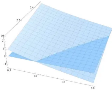
Figure 2.3.1 The implicit function visible at z = 0
The horizontal axes plotx1 and, to the back,x2:The vertical axis plotsz:The
increas-ing surface depicts the graph of the functionz =g(x1; x2) b: When this surface crosses
the horizontal plane at z = 0; a curve is created which contains all the points where
z = 0:Looking at this curve illustrates that the functionz = 0,g(x1; x2) =b implicitly
de…nes a function x2 =h(x1): See exercise7 for an explicit analytical derivation of such
an implicit function. The derivative dx2=dx1 is then simply the slope of this curve. The
analytical expression for this is - using (2.3.3) -dx2=dx1 = (@g(:)=@x1)=(@g(:)=@x2):
First-order conditions of the maximization problem
The maximization problem we obtained in (2.3.2) is an example for the substitution method: The budget constraint was solved for one control variable and inserted into the objective function. The resulting maximization problem is one without constraint. The problem in (2.3.2) now has a standard …rst-order condition,
dF dx1
= @F
@x1
+ @F
@x2 dh dx1
= 0: (2.3.4)
Taking into consideration that from the implicit function theorem applied to the con-straint,
dh dx1
= dx2
dx1
= @g(x1; x2)=@x1
@g(x1; x2)=@x2
; (2.3.5)
the optimality condition (2.3.4) can be written as @x@F 1
@F=@x2
@g=@x2
@g(x1;x2)
@x1 = 0: Now de…ne the Lagrange multiplier @F=@x2
@g=@x2 and obtain
@F @x1
@g(x1; x2) @x1
As can be easily seen, this is the …rst-order condition of the Lagrangian
L=F(x1;x2) + [b g(x1;x2)] (2.3.7)
with respect to x1:
Now imagine we want to undertake the same steps forx2;i.e. we start from the original
problem (2.3.1) but substitute out x1: We would then obtain an unconstrained problem
as in (2.3.2) only that we maximize with respect to x2: Continuing as we just did for x1
would yield the second …rst-order condition
@F @x2
@g(x1; x2) @x2
= 0:
We have thereby shown where the Lagrangian comes from: Whether one de…nes a La-grangian as in (2.3.7) and computes the order condition or one computes the …rst-order condition from the unconstrained problem as in (2.3.4) and then uses the implicit function theorem and de…nes a Lagrange multiplier, one always ends up at (2.3.6). The Lagrangian-route is obviously faster.
2.3.2
Shadow prices
The idea
We can now also give an interpretation of the meaning of the multipliers . Starting from the de…nition of in (2.3.6), we can rewrite it according to
@F=@x2 @g=@x2
= @F
@g =
@F @b:
One can understand that the …rst equality can “cancel” the term @x2 by looking at the
de…nition of a (partial) derivative: @f(x1;:::;xn)
@xi =
lim4xi!0 f(x1;:::;xi+4xi;:::;xn) f(x1;:::;xn)
lim4xi!0 4xi : The
2.3. The idea behind the Lagrangian 25
A derivation
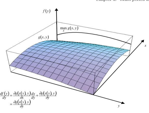
A more rigorous derivation is as follows (cf. Intriligator, 1971, ch. 3.3). Compute the derivative of the maximized Lagrangian with respect to b,
@L(x1(b); x2(b))
@b =
@
@b(F(x1(b); x2(b)) + (b) [b g(x1(b); x2(b))]
=Fx1
@x1 @b +Fx2
@x2
@b +
0
(b) [b g(:)] + (b) 1 gx1
@x1 @b gx2
@x2 @b
= (b)
The last equality results from …rst-order conditions and the fact that the budget constraint holds.
As L(x1; x2) =F(x1; x2) due to the budget constraint holding with equality,
(b) = @L(x1; x2)
@b =
@F(x1; x2)
@b
An example
The Lagrange multiplier is frequently referred to as shadow price. As we have seen, its unit depends on the unit of the objective function F: One can think of price in the sense of a price in a currency, for example in Euro, only if the objective function is some nominal expression like pro…ts or GDP. Otherwise it is a price expressed for example in utility terms. This can explicitly be seen in the following example. Consider a central planner that maximizes social welfare u(x1; x2) subject to technological and resource
constraints,
maxu(x1; x2)
subject to
x1 =f(K1;L1); x2 =g(K2;L2); K1+K2 =K; L1 +L2 =L:
Technologies in sectors 1 and 2 are given by f(:) and g(:) and factors of production are capital K and labourL: Using as multipliersp1; p2; wK and wL; the Lagrangian reads
L=u(x1; x2) +p1[f(K1;L1) x1] +p2[g(K2; L2) x2]
+wK[K K1 K2] +wL[L L1 L2] (2.3.8)
and …rst-order conditions are
@L @x1
= @u
@x1
p1 = 0; @L @x2
= @u
@x2
p2 = 0; (2.3.9)
@L @K1
=p1 @f @K1
wK = 0; @L @K2
=p2 @g @K2
wK = 0;
@L @L1
=p1 @f @L1
wL= 0; @L @L2
=p2 @g @L2
Here we see that the …rst multiplierp1 is not a price expressed in some currency but the
derivative of the utility function with respect to good1, i.e. marginal utility. By contrast, if we looked at the multiplierwK only in the third …rst-order condition,wK =p1@f =@K1;
we would then conclude that it is a price. Then inserting the …rst …rst-order condition,
@u=@x1 =p1;and using the constraintx1 =f(K1;L1)shows however that it really stands
for the increase in utility when the capital stock used in production of good 1rises,
wK =p1 @f @K1
= @u
@x1 @f @K1
= @u
@K1 :
Hence wK and all other multipliers are prices in utility units.
It is now also easy to see that all shadow prices are prices expressed in some currency if the objective function is not utility but, for example GDP. Such a maximization problem could read maxp1x1 +p2x2 subject to the constraints as above. Finally, returning to
the discussion after (2.1.5), the …rst-order conditions show that the sign of the Lagrange multiplier should be positive from an economic perspective. If p1 in (2.3.9) is to capture
the value attached tox1in utility units andx1 is a normal good (utility increases inx1;i.e. @u=@x1 >0), the shadow price should be positive. If we had represented the constraint in
the Lagrangian (2.3.8) asx1 f(K1;L1)rather than right-hand side minus left-hand side,
the …rst-order condition would read @u=@x1+p1 = 0 and the Lagrange multiplier would
have been negative. If we want to associate the Lagrange multiplier to the shadow price, the constraints in the Lagrange function should be represented such that the Lagrange multiplier is positive.
2.4
An overlapping generations model
We will now analyze many households jointly and see how their consumption and saving behaviour a¤ects the evolution of the economy as a whole. We will get to know the Euler theorem and how it is used to sum factor incomes to yield GDP. We will also understand how the interest rate in the household’s budget constraint is related to marginal produc-tivity of capital and the depreciation rate. All this jointly yields time paths of aggregate consumption, the capital stock and GDP. We will assume an overlapping-generations structure (OLG).
2.4. An overlapping generations model 27
2.4.1
Technologies
The …rms
Let there be many …rms who employ capital Kt and labour L to produce output Yt
according to the technology
Yt=Y (Kt; L): (2.4.1)
Assume production of the …nal good Y (:) is characterized by constant returns to scale. We choose Yt as our numeraire good and normalize its price to unity, pt = 1: While this
is not necessary and we could keep the price pt all through the model, we would see that
all prices, like for example factor rewards, would be expressed relative to the price pt:
Hence, as a shortcut, we setpt = 1:We now, however, need to keep in mind that all prices
are henceforth expressed in units of this …nal good. With this normalization, pro…ts are given by t =Yt wKt Kt wLtL. Letting …rms act under perfect competition, the
…rst-order conditions from pro…t maximization re‡ect the fact that the …rm takes all prices as parametric and set marginal productivities equal to real factor rewards,
@Yt
@Kt
=wtK; @Yt
@L =w
L
t: (2.4.2)
In each period they equatet; the marginal productivity of capital, to the factor pricewKt
for capital and the marginal productivity of labour to labour’s factor reward wL t.
Euler’s theorem
Euler’s theorem shows that for a linear-homogeneous function f(x1; x2; :::; xn) the
sum of partial derivatives times the variables with respect to which the derivative was computed equals the original function f(:);
f(x1; x2; :::; xn) =
@f(:)
@x1 x1+
@f(:)
@x2
x2 +:::+ @f(:)
@xn
xn: (2.4.3)
Provided that the technology used by …rms to produce Yt has constant returns to scale,
we obtain from this theorem that
Yt=
@Yt
@Kt
Kt+
@Yt
@LL: (2.4.4)
Using the optimality conditions (2.4.2) of the …rm for the applied version of Euler’s theorem (2.4.4) yields
Yt=wtKKt+wLtL: (2.4.5)
Total output in this economy,Yt;is identical to total factor income. This result is usually
2.4.2
Households
Individual households
Households live again for two periods. The utility function is therefore as in (2.2.1) and given by
Ut= lncyt + (1 ) lncot+1: (2.4.6)
It is maximized subject to the intertemporal budget constraint
wLt =cyt + (1 +rt+1) 1cot+1:
This constraint di¤ers slightly from (2.2.2) in that people work only in the …rst period and retire in the second. Hence, there is labour income only in the …rst period on the left-hand side. Savings from the …rst period are used to …nance consumption in the second period.
Given that the present value of lifetime wage income is wL
t; we can conclude from
(2.2.4) and (2.2.5) that individual consumption expenditure and savings are given by
cyt = wtL; cot+1 = (1 ) (1 +rt+1)wLt; (2.4.7)
st=wtL c y
t = (1 )w
L
t: (2.4.8)
Aggregation
We assume that in each period L individuals are born and die. Hence, the number of young and the number of old is L as well. As all individuals within a generation are identical, aggregate consumption within one generation is simply the number of, say, young times individual consumption. Aggregate consumption in t is therefore given by
Ct=Lcyt+Lcot:Using the expressions for individual consumption from (2.4.7) and noting
the index t (and not t+ 1) for the old yields
Ct=Lcyt +Lc o
t = w
L
t + (1 ) (1 +rt)wtL1 L:
2.4.3
Goods market equilibrium and accumulation identity
The goods market equilibrium requires that supply equals demand, Yt = Ct+It; where
demand is given by consumption plus gross investment. Next period’s capital stock is - by an accounting identity - given byKt+1 =It+(1 )Kt:Net investment, amounting to the
change in the capital stock, Kt+1 Kt, is given by gross investmentItminus depreciation
Kt, where is the depreciation rate,Kt+1 Kt=It Kt. Replacing gross investment
by the goods market equilibrium, we obtain the resource constraint
Kt+1 = (1 )Kt+Yt Ct: (2.4.9)
For our OLG setup, it is useful to rewrite this constraint slightly ,