Equality of educational opportunity employing Pisa data: taking both achievement and access into account

!"#

$ %

& & #

'(#

Equality of educational opportunity employing PISA data:

Taking both achievement and access into account

Márcia de Carvalho*

Departamento de Estatística and Centro de Estudos sobre Desigualdade e Desenvolvimento (CEDE), Federal Fluminense (UFF), Brazil.

Luis Fernando Gamboa∗∗

Facultad de Economía, Universidad del Rosario

Fábio D. Waltenberg***

Departamento de Economia and Centro de Estudos sobre Desigualdade e Desenvolvimento (CEDE), Universidade Federal Fluminense (UFF), Brazil.

Abstract

While PISA datasets have been used for measuring inequality of educational opportunity they have important limitations: (i) samples only cover a relatively limited fraction of developing countries’ cohorts of 15-year-olds, and (ii) such fractions are not uniform across countries and waves. This casts doubts on the reliability of such measures when used for international and intertemporal comparisons: a milder calculated inequality of opportunity in a given country at a given moment might simply be the artifact of a more restricted and homogeneous sample. Previous attempts of addressing this problem have focused on explicitly reconstructing full samples. Here an alternative path is followed, relying on bidimensional indices, in which equality of opportunity in achievement is the first dimension and equality of opportunity for access to the exam is the second one. We compute the two dimensions and aggregate them using alternative techniques. Employing PISA 2006/2009 data for six Latin-American countries we observe rank reversals when comparing results based upon our indices and those based upon conventional indices of equality of opportunity for achievement. We then generalize our approach allowing for more dimensions and parameterizing the dimensions’ weights.

Resumen

La medición de la desigualdad de oportunidades con las bases de PISA implican varias limitaciones: (i) la muestra sólo representa una fracción limitada de las cohortes de jóvenes de 15 años en los países en desarrollo y (ii) estas fracciones no son uniformes entre países ni entre periodos. Lo anterior genera dudas sobe la confiabilidad de estas mediciones cuando se usan para comparaciones internacionales: mayor equidad puede ser resultado de una muestra más restringida y más homogénea. A diferencia de enfoques previos basados en reconstrucción de las muestras, el enfoque del documento consiste en proveer un índice bidimensional que incluye logro y acceso como dimensiones del índice. Se utilizan varios métodos de agregación y se observan cambios considerables en los rankings de (in) equidad de oportunidades cuando solo se observa el logro y cuando se observan ambas dimensiones en las pruebas de PISA 2006/2009. Finalmente se propone una generalización del enfoque permitiendo otras dimensiones adicionales y otros pesos utilizados en la agregación.

JEL Classification: I24, O54.

Keywords: equality of opportunity, measurement of inequality of opportunity, multidimensional measures, PISA test scores, Latin America.

ξ _{The authors would like to thank attendants of seminars at Universidade de São Paulo, Universidade Federal}

Fluminense in Niterói, Brazil, and at the ZEW Workshop on “Equality of Opportunity in Education” in Mannheim, Germany, particularly to Erwin Ooghe and Johannes Kunz. We are very grateful to Jérémie Gignoux for having provided his Stata code used in calculating the index of equality of opportunity in achievement. Finally, we thank CNPq/UFF (“Programa de Iniciação Científica”) and the Universidad del Rosario for providing funds for research assistance.

* _{E-mail address: [email protected].}

1. Introduction

A liberal-egalitarian theory of justice that has been widely discussed in recent years is

that of “equality of opportunity” (EOp), popularized among economists by John Roemer,

according to which while inequalities due to different circumstances are intolerable,

inequalities due to choices made by the individuals are acceptable (Roemer, 1998). Different

methodologies have been proposed attempting to translate the theory into measuring

procedures in order, for example, to determine how far apart countries or regions stand from

an ideal of equality of opportunity in terms of, say, income distribution (e.g., Checchi &

Peragine, 2010; Dunnzlauf et al. 2010). Two recent extensive surveys are available

documenting the vast literature produced along the last ten years or so (Pignataro, 2012;

Ramos & Van de Gaer, 2012).

Measuring inequality of opportunity in the educational sphere has been the focus of

recent contributions, which concentrate either on opportunity for access to a given level of

studies (e.g., Paes de Barros et al. 2009; Vega et al. 2010), or on opportunity in terms of

educational achievement (e.g., Checchi & Peragine, 2005; Ferreira & Gignoux, 2011; Gamboa &

Waltenberg, 2012). In this paper we combine both concerns.

Pupils’ educational achievement is usually measured by standardized test scores, such

as those made available by OECD’s Programme for International Student Assessment (PISA),

which are taken to be proxies for the knowledge and basic skills pupils possess in different

areas: reading, mathematics, or sciences. While PISA datasets present many well-known

virtues, they are also plagued by some important limitations, particularly in terms of coverage

rates of the population of individuals whose age is 15 (the exam’s focus). The reasons for not

evaluating individuals include: their being not enrolled in schools, their being enrolled in very

low grades, logistic difficulties in the application of the test, and school-level exclusions related

to pupils’ physical or intellectual deficiencies. While in developed countries, the coverage rate

is systematically larger than 80% – sometimes approaching 100% –, the samples cover a

relatively limited fraction of developing countries’ cohorts of 15-year-olds. Moreover such

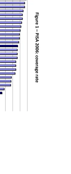
fractions are not uniform across countries and PISA waves (see Figures 1 and 2).

< Figures 1 and 2 around here >

These sample limitations cast doubts on the reliability of indices of inequality of

educational opportunities concerning developing countries, let alone international and

at a given moment) might simply be the artifact of a more restricted sample – possibly more

homogeneous – as compared to that of another country (or another moment).

Previous attempts of addressing this issue have been ingeniously performed by

Ferreira & Gignoux (2011), who have tried to explicitly reconstruct a full sample, but have

encountered two obstacles. First, the need to handle simultaneously many ancillary national

datasets, (possibly) dissimilar in many respects, contrary to PISA datasets themselves, which

are designed to be comparable across countries and years. Second, the need to adopt strong

assumptions in order to assign scores to missing pupils in the simulated distribution of scores

that they construct trying to mimic the actual distribution of scores that would have been

observed had pupils representing the whole cohort taken the exam.

Our strategy is of a very different nature. Instead of dealing with less-than-full

coverage by attempting to reconstruct a full sample, we take it for granted that it is not

possible to obtain a reliable and uncontroversial reconstructed full sample. We prefer to

explicitly acknowledge that there are two different dimensions of opportunity – access to PISA

exams and achievement conditional on access. We then introduce a bidimensional index of

equality of opportunity composed of the (conditional-on-access-) achievement dimension and

the access (-to-PISA) dimension. For the first dimension, we compute conventional inequality

of opportunity in test scores. Following Ferreira & Gignoux (2011), we propose the proportion

of the variance in test scores which is explained by variables reflecting pupils’ circumstances.1

As for the second dimension, we employ two different methods, the first of which is based on

each country’s reported PISA’s coverage rate, while the second relies on Paes de Barros et al.’s

(2009) Human Opportunity Index (HOI).

Needless to say that both dimensions are important for those worried about inequality

of opportunities. Yet it seems to us that access to a given advantage (which here means taking

part in PISA exam) is even more pressing and crucial than the relative performance obtained

by those individuals for which such advantage is accessible (which here stands for their test

scores).2 The prominence of EOp in access with respect to EOp in achievement accentuates the

importance of taking into account the former and not restricting the analysis to the latter.

Whatever the relative importance attributed to each dimension of EOp it is necessary

to aggregate the dimensions. We do so by means of two different techniques: either using a

1 _{Based on Item Response Theory (IRT), answers given by pupils to exam questions are transformed into test scores}

and arbitrarily standardized to exhibit a given mean and a given standard deviation. As explained in detail by Ferreira & Gignoux (2011), because of this procedure, many usual inequality indices are not ordinally invariant, which led them to recommend the use of the variance to compute inequality of educational achievement, and the fraction of the variance explained by circumstances to compute inequality of opportunity in educational achievement.

2 _{Such “hierarchical view” we suggest here which prioritizes EOp in access with respect to EOp in achievement has}

simple multiplicative specification, or turning to fuzzy sets transformations, which are routine

in multidimensional poverty analysis when it comes to aggregating variables expressed in

different metrics (Cerioli & Zani, 1990;Cheli & Lemmi, 1995;Lemmi & Betti, 2006).

In addition to overcoming the limitations of measuring EOp in education with an

exclusive focus on the achievement dimension – which per se might lead to misestimating

inequality of educational opportunity in some countries – some (though not all) of the versions

of the index we introduce also present the attractive feature of economizing on data

requirements, since they only involve PISA data complemented by descriptive information

contained in PISA technical reports.

We illustrate our approach for six Latin-American countries that took part in PISA 2006

and 2009, observing that ranking those six countries according to different versions of the

bidimensional index we introduce differs from ranking them according to a conventional index,

exclusively focused on achievement-EOp.

We skip a thorough presentation of equality of opportunity theory, as well as the main

controversies around measuring issues, since we believe that will be redundant with the

available literature, covered by two recent surveys already mentioned in this introductory

Section 1 (Pignataro, 2012; Ramos & Van de Gaer, 2012). The remaining of the paper is

organized around five further sections. Section 2 is devoted to explaining the original

motivation for this study, namely, PISA’s coverage rate problem, as well as previous attempts

of addressing it. In Section 3 we uncover our approaches to the problem, which amounts to

calculating bidimensional indices of equality of educational opportunities, taking into account

both achievement in PISA and access to PISA – each of which if taken alone would provide an

incomplete picture of the prevalent degree of inequality of educational opportunity. Section 4

contains an illustration for six Latin-American countries that took part in PISA 2006 and 2009,

comparing rankings of inequality of educational opportunity for those countries as calculated

by the indices we introduce with rankings obtained from a conventional index. We observe

rank reversals, suggesting that disregarding the access dimension has consequences. In Section

5 we undertake a generalization of our approach, allowing for more dimensions and

parameterizing the dimensions’ weights. We conclude in Section 6, pointing out possible

future research paths.

2. PISA’s coverage rate problem: paths and attempts to circumvent biases

OECD’s PISA datasets have been collected every three years, starting in 2000, allowing

over-time comparability. The fourth wave, collected in 2009, is the most recent which is

representative samples of students in dozens of countries in three different subjects –

mathematics, sciences and reading – as well as detailed information on students' background

and schools' personnel and functioning conditions. The fourth wave, for example, contains

samples of about 520 thousand students representing around 28 million pupils of more than

70 countries (OECD, 2012: 25).

Two related limitations that affect PISA samples should be mentioned. First,

individuals who are enrolled in a very low grade (“grade 6” or below3) or who are not enrolled

in schools are not assessed by PISA – they are “ineligible”. Another set of eligible pupils does

not take the exam for logistic or fortuitous reasons (e.g., pupils living in a remote region, or

pupils who were sick in the day the exam took place). Finally, local managers of PISA exams

might also exclude some pupils for physical or intellectual deficiencies (the accepted cases are

carefully detailed in PISA manuals). As a consequence of these exclusions empirical findings

based on PISA data should not be taken as valid for cohorts of 15-year-old individuals, but

rather as valid for teenagers represented by a sample of pupils who: (i) have stayed in the

educational system, (ii) have not repeated too many grades, (iii) being eligible, have actually

been evaluated.

The second limitation is a corollary of the first: the proportion of the cohort of

15-year-old individuals which has been excluded is not uniform across countries or in a given country

over time. As shown in figures 1 and 2, differences can be substantial – spatially or temporally

– casting doubts on the reliability of cross-country comparisons, as well as on over-time

evaluations.

As an example, let us reproduce here coverage rates for six Latin-American countries

recently studied (Gamboa & Waltenberg, 2012) and to which we too turn to in the illustration

provided below. In 2006, the rates are: Argentina (79%), Brazil (55%), Chile (78%), Colombia

(60%), Mexico (54%) and Uruguay (69%); in 2009, they are: Argentina (69%), Brazil (63%), Chile

(85%), Colombia (59%), Mexico (61%) and Uruguay (63%). These figures reveal that: (i) the

coverage rates are not particularly high on average, (ii) although all countries come from the

same region, cross-country dispersion is substantial, with a range of around 25 percentage

points in both years, (iii) there are important oscillations for given countries across waves

(ranging from -10 to +8 percentage points).

Disregarding coverage rates – which are incomplete and variable across countries and

over time – might lead to an imprecise estimation of the level of unfair inequalities in some

countries, particularly those with smaller coverage rates. For example, if Mexico turns out to

3 _{PISA’s “grade 6” corresponds with different names in different countries. PISA technical reports (e.g., OECD, 2009}

show lower inequality of opportunity in achievement than Argentina in 2006, one might

wonder whether such result actually reflects larger unfair educational achievement inequality

in the latter than in the former, or whether the result is driven by a more homogeneous

sample in Mexico (the country that has the lowest coverage rate in that year) than in

Argentina (the one with the highest rate).4

It is important to emphasize that the issue of access that we raise here is not a minor

technical problem, but instead a crucial one for those worried about widening opportunities

for all. In a sense, as expressed by Paes de Barros et al. (2009) and reinforced by Peragine

(2010), lack of access to a given advantage (which here means “not being able to take part in

PISA exams”) is even more primary and serious for those concerned with equality of

opportunity than the relative performance obtained by individuals for which such advantage is

accessible (that is, their test scores). In other words, while underperforming in PISA might

signal future difficulties in an individual’s life, not even been eligible to the exam is probably

correlated with much more considerable obstacles in the future. Also, while once again both

dimensions of inequality of opportunity might pose problems for future generations, the lack

of access is arguably more pressing.

To address PISA coverage problems, we view at least three alternative paths, two of

which are mentioned in this section. The third path is the one we adopt in this study, and its

(longer) explanation is reserved to the next section.

The first path is simply to be cautious when interpreting the results of any study that

employs PISA for developing countries. This is the humblest path, but also the riskiest, since

many readers (and possibly policymakers) might basically overlook the call for caution, and

judge results by their face value. Gamboa & Waltenberg (2012) opt for what here we call “first

path”, presenting results based on PISA limited samples and emphasizing that caution is

necessary in their interpretation. 5

A second path consists of explicitly reconstructing full samples. Recently Ferreira &

Gignoux (2011) have done so for four countries: Brazil, Indonesia, Mexico, and Turkey. Due to

the absence of information in PISA samples about non-participant pupils, it is not possible to

perform a correction such as Heckman's familiar procedure. Instead, they have turned to

4 _{In Colombia, in turn, a considerable dropout rate has been observed during the 1990s, for multiple reasons among}

which: economic recession (reducing enrollment in private schools); increase in the standards necessary to be promoted from grade to grade; negative externalities caused by the domestic conflicts. This trend was reverted during the last decade mainly as a consequence of multiple public policies designed to reduce demand barriers. The more recent situation potentially reduces the biases of estimations of equity based on PISA or national standardized tests.

5 _{Additionally, as a sensitivity analysis the authors report a simple simulation taking the country showing the lowest}

ancillary databases (i.e. household surveys), which, however, do not contain information on

test scores. They have then imposed some assumptions in order to undertake two different

kinds of simulation. The first one consists of re-weighting test scores observations in PISA

datasets by means of information taken from the ancillary databases on the fraction of

different types of individuals in the population.6 The second one consists of imputing into the

dataset pupils who were not evaluated, ascribing to them scores equal to the lowest score

obtained by individuals very similar to them – namely, those pertaining to the same “type”,

where type is defined following Roemer (1998).

The first simulation, which relies on more conventional assumptions, provides results

almost equal to the original results, both in terms of inequality of achievement and of

opportunities. While such somewhat unexpected finding might offer relief for those employing

PISA datasets, it is not excluded that applying the procedure to other countries/years could

lead to more substantial changes. The second simulation results in more substantial

differences with respect to the naïve calculations. Having said that, the latter technique has a

drawback which is particularly important when it comes to undertaking international and

intertemporal comparisons, namely, the fact that it requires handling many different

country-specific survey datasets, and choosing similar variables in all of them, which might not always

be possible or might lead to poor definitions of types. Another disadvantage is that the

criterion employed to input pupils and their scores into the dataset is controversial – Ferreira

& Gignoux (2011) themselves acknowledge that, stating that their assumptions are

“admittedly extreme”.

Their pioneering effort deserves to be praised, and we would like to view it as

complementary to our approach, not substitute. Yet we believe sample corrections of PISA

data still present high costs (especially being data-intensive) and limited benefits (unstable

results; small impacts or results based on strong assumptions). For these reasons we tend to

favor a third path, which is described below.

3. A bidimensional approach: taking both achievement and access into account

Our strategy is of a very different nature. Instead of dealing with less-than-full

coverage by attempting to, so to speak, “reconstruct a full coverage”, we take it for granted

that it is not possible to obtain a reliable and uncontroversial reconstructed full sample. We

prefer to explicitly acknowledge that there are two different dimensions of opportunity –

access (to PISA exams) and achievement (conditional on access), to measure them separately

and to aggregate them somehow, as explained below.

1. Dimension 1: inequality of opportunity in achievement. We restrict the calculation of

inequality of opportunity in achievement to the available PISA samples, which as

stated above represent only a fraction of each country’s 15-year-olds. To do so, we

employ Ferreira & Gignoux’s (2011) regression-based index of inequality of

educational opportunity (hereafter: IOFG), which is calculated as the proportion of the

variance of test scores that is explained by a set of circumstances, with 0 ≤ IOFG ≤ 1,

thus ranging from 0 (perfect equality of opportunity) to 1 (perfect inequality of

opportunity). In our approach, again following Ferreira & Gignoux (2011), the set of

circumstances includes: mother and father education, father occupation, stock of

educational capital, city size and ownership of specific durables.7 That provides us with

a valuable, albeit limited, piece of information upon which we can judge and compare

countries’ educational systems.8

2. Dimension 2: inequality of opportunity in access. We have to take into account the

proportion of individuals which are actually represented in a given country’s PISA

sample, in order to sanction countries according to how far apart they stand from full

coverage. To do so, we propose two methods:

a) The first one consists of simply employing coverage rates available in PISA

technical reports, which range from 0 (no coverage) to 1 (full coverage), as the

second dimension of our index. Following the notation employed in a related

literature9 we denote the overall coverage rate by p, with 0 ≤p≤ 1.

b) The second one is more involved, but intuitive too. It consists of taking into

account not only the overall coverage rate for each country as in (a) above, but

also the coverage rate for different types of a given population, which might vary

across types (e.g., across types defined according to gender and ethnicity). In that

we follow Paes de Barros et al. (2009), who compute what they label a “Human

Opportunity Index” (HOI), as follows: HOI = p.(1−D), where:pis defined and bounded as above; 0 ≤ D ≤ 1 stands for a dissimilarity index, which aggregates the

7 _{A good property of this index is the ease with which it is calculated: it is simply the R-squared of the estimation of}

scores regressed against the set of circumstances cited above. Another virtue is related to a characteristic of the R-squared: since it never goes down when new variables are added to the regression, we can interpret it in the present context as a lower bound of inequality of opportunity for achievement: if further variables reflecting circumstances could be added (but are unobservable, for example), we can be sure that the index would either remain stable or go up. For a thorough discussion, see Ferreira & Gignoux (2011).

8 _{It should be mentioned at this point that although we employ a regression, we are not attempting to establish}

causality. The exercise undertaken is essentially a static decomposition of inequality (as expressed by the variance) into unfair inequality (the R-squared) and fair inequality (1-R²).

difference between the average coverage ratepand each type’s coverage rate

weighted by the relative frequency of each type in the population (where type is

understood according to Roemer’s (1998) meaning), and with 0 ≤ HOI ≤ 1. Such

index could be viewed as one which expresses opportunity for access, both for the

population taken together and for specific groups (types).

The main advantages of method (a) above are its simplicity, the ease with which

information can be gathered (available in PISA reports) and the fact that it does not require

further datasets, what is important for those willing to make international-intertemporal

comparisons. The main advantage of method (b), in turn, is that it is not mute with respect to

cross-types differential opportunities.10

3. Aggregating the two dimensions. The remaining step is to aggregate the two

dimensions into one single index, which we generically call the “Bidimensional Index of

Equality of educational opportunity” (or BIE). We work with two aggregation

procedures: a direct multiplicative specification, and the fuzzy sets technique. Since we

also have two procedures for calculating the access dimension, we obtain four versions

of our index (BIEV, with V = 1, …, 4). These four procedures are described below in

subsections 3.1-3.4.

3.1. BIE1: access as overall coverage rate; aggregation in a simple multiplicative form

An interesting way of dealing with both dimensions – achievement and access –, is to

weigh the inverse of IOFG by p, that is:

(

)

EOp t achievemen

FG EOp

access

IO p

BIE

− −

− ⋅

= 1

1 (3.1)

with: 0 <p≤ 1, 0 ≤ IOFG< 1, 0 < BIE1 ≤ 1.

Clearly, the index is increasing in pand decreasing in IOFG as would be desirable. More

interesting is to consider some limiting cases for its attributes. First, since IOFG ranges in the

interval [0,1), with 0 standing for perfect equality of opportunity in achievement, (1 – IOFG) will

equal 1 in the case where circumstances are unrelated to outcomes for those pupils who have

taken PISA exams. In such limiting case, BIE1 will depend solely upon the coverage rate: the

10 _{The use of HOI – as opposed to Yalonetsky’s (2012) recently proposed dissimilarity index – is endorsed both by}

higher it is, the larger will be the opportunities offered to 15-year-olds of a given country.

Conversely, in a case of full coverage, where p= 1, the index BIE1 will depend solely upon

inequality of opportunity in achievement.BIE1 can also be expressed through a penalty, P, on

the fact that coverage is less than full: BIE₁= p⋅

(

)

3.2. BIE2: access as overall coverage rate; aggregation through the fuzzy sets technique

A second way of dealing with the two dimensions is routine in multidimensional

poverty analysis. It consists of standardizing observations expressed in each dimension’s

metric by means of the fuzzy sets technique and then aggregating them additively (with

certain weights) to generate BIE2.

The fuzzy function of a given variable (x1) from country i will be a linear variation

between minimal and maximal values, as follows (Cerioli & Zani, 1990; Cheli & Lemmi, 1995):

       = < < − − = = max , 1 max min , min max min min , 0 ) ( 1 , 1 , 1 , 1 , 1 , i i i i i x if x if x x if x

f (3.2)

This applies, for example, to the coverage rate variable, p, where the larger it is, the

better it is (i.e., the index should be increasing in p). A similar function is defined but with

inverted minimal and maximal values, for the fuzzy set of another variable (x2):

       = < < − − = = min , 1 min max , min max max max , 0 ) ( 2 , 1 , 2 , 2 , 2 , i i i i i x if x if x x if x

f (3.3)

This applies, for example, to the inequality index, IOFG, where the larger it is, the worse

it is (i.e., the index should be decreasing in IOFG). The next step is weighing the two dimensions.

We postpone a discussion about weights to Section 5 and here, as a first approach, we simply

consider the simplest solution of attributing an equal weight to each dimension:

2 ) ( )

( 1 2

2 EOp t achievemen EOp access x f x f BIE − − +

With respect to BIE1, a disadvantage of BIE2 is that the calculated values will depend

upon the countries used in the sample, since minimal and maximal values in the sample

determine the function. The main advantage of the fuzzy method is that in a more general

context (i.e., a multidimensional one) it allows to transform distributions which do not fit the

range [0-1] to one that fits, a point to which we come back in Section 5.

3.3. BIE3: access as HOI; aggregation in a simple multiplicative form

A third version of the index relies on HOI – which, as argued before, can be viewed as

an “opportunity-for-access index” – to express the access dimension. The achievement

dimension remains as it was before:

(

)

EOp t achievemen FG EOp

access

IO HOI

BIE

− −

− ⋅

= 1

3 (3.5)

with: 0 < HOI ≤ 1, 0 ≤ IOFG< 1, 0 < BIE3 ≤ 1.

And sinceHOI= p.(1−D), we can rewrite (3.5) as:

(

)

EOp t achievemen

FG

EOp access

types across overall

IO D

p BIE

− −

−

− ⋅ −

= .(1 ) 1

3 (3.6)

with: 0 <p≤ 1, 0 ≤ D < 1, 0 ≤ IOFG< 1, 0 < BIE3 ≤ 1.

Now we have an index which is once again decreasing in IOFG (which captures

inequality of opportunity in achievement), increasing in p(which captures the average

access-to-PISA in a given country) but additionally it is also decreasing in D (which captures

cross-groups inequality of opportunity in access-to-PISA). A broader range of interesting cases

emerge, such as those we emphasize below:

a) If a country presents full coverage, we will havep=1 but alsoD=0 (access will be 100% for each type). Then, BIE1 will depend solely upon inequality of

opportunity in achievement. Such case is relevant for advanced countries, where

the coverage rate in PISA approaches 100%, such as Switzerland or Canada in 2006

(Figure 1). However, that is not what is observed in most countries, let alone

developing countries, but it is implicitly assumed in conventional calculations of

b) A country could have perfect equality of opportunity in achievement (IOFG = 0),

such that BIE3 would depend exclusively upon access. Such second dimension

would depend upon two subdimensions: the overall coverage rate,p, and the

cross-types dissimilarity in coverage rates, D.

c) Two countries could show similar inequality of opportunity in achievement, OFG, as

well as similar coverage rates,p, but could differ in terms of their relative

cross-types dissimilarity with respect to access. Such case might apply to pair-wise

comparisons of equality of opportunity among countries from a given region.

3.4. BIE4: access as HOI; aggregation through the fuzzy sets technique

Finally, and for the sake of completeness, we mention the version BIE4, which would

standardize HOI as in Equation (3.2), and aggregate the dimensions as in Equation (3.4). Pros

and cons are those described in Subsection 3.2.

4. An illustration of the methodology: EOp in Latin America

In this section, we provide an illustration of our approach for six Latin-American

countries that took part in PISA 2006 and 2009. We compare the rankings of inequality of

educational opportunity for those countries as calculated by two versions of the bidimensional

index introduced here (BIE1 and BIE2) 11

with the ranking obtained from a conventional index

that only takes into account inequality of opportunity for achievement. Regarding test scores,

we employ PISA’s “plausible values” for Mathematics.

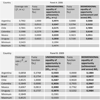
We start with results using the first technique (BIE1) reported in Table 1 and Figure 3.

< Table 1 around here >

Figure 3 clearly reveals that both in 2006 and in 2009 rank reversals are observed

when switching from an index of equality of opportunity that focuses exclusively on

achievement (1 – IOFG) to a more complete index that encompasses both equality of

opportunity in achievement and in access (BIE1).

12

For example, Argentina is the most

opportunity-unequal country in 2006 in terms of achievement, but after taking into account its

relatively good coverage rate, it moves to the third position. Chile also moves up, from the

third position to the first position. Colombia and Mexico – countries that have low coverage

11 _{In a companion paper, we are working in calculating estimates of BIE}

3 and BIE4.

12 _{Since samples are not very large, differences in rakings should be handled with caution: the difference between two}

rates – do the opposite movement, from first and fourth to third and sixth, respectively. In

2009, Brazil and Chile, as well as Colombia and Mexico exchange positions when we switch

from the ranking based on unidimensional equality of opportunity to the one based on a

bidimensional equality of opportunity.

< Figure 3 around here >

For presentational purposes, it is useful to observe our results amidst iso-opportunity

curves (Barros et al., 2009), which have been plotted in Figure 4 exclusively for PISA 2006.

Brazil and Mexico, below the curve “BIE1=0,4” are to be contrasted to Chile, above the curve

“BIE1=0,5”. More interesting is to compare Argentina and Colombia: while the former performs

relatively well in the access-EOp dimension and does not fare very well in the

achievement-EOp dimension, the latter presents the opposite situation.

< Figure 4 around here >

Results obtained using the second version of the index (BIE2) appear in Table 2. The

same rank reversals are observed. In fact, the correlation between calculated values for BIE2

and BIE2 is 0,97, turning the second version redundant at this point.

< Table 2 around here >

5. Generalizing the approach: Further dimensions and varying weights

It is a natural step to generalize our approach, allowing both for more dimensions and

for different weights for each dimension. The intuition is that when we use such bidimensional

indices, we are in fact:

(i) Defining social welfare functions – or, more precisely in this context: “equality of

opportunity functions” – based upon certain attributes, BIE = f (EOp in access, EOp in

achievement). However, other attributes could be incorporated. Although we

presented BIE3 as a bidimensional index in which one of the dimensions is subdivided

in two subdimensions, we were already hinting in fact on three dimensions:p, (1 – D),

and (1 - IOFG). More generally, the index could be multidimensional.

(ii) Working with implicit weights and thus ad hoc trade-offs between the two (now

5.1. A multidimensional index

Average scores might be a relevant dimension of equality of educational opportunities.

Worried about the quality of education of second-generation immigrants in OECD countries,

Kunz (2012) is particularly concerned with those living in Germany, whose average score in

reading in PISA 2009 is 474. However such indeed worrying result is in fact much better than

the average score in any Latin American country in that year, where the highest average score

is Chile’s (449). So while second-generation immigrants are in a very bad relative position in

the German context, in absolute terms the German schooling system provides more

opportunity to that worse-off group for acquiring knowledge and basic skills than

Latin-American schooling systems provide to their average pupils. That might be viewed as a

dimension of opportunity too: ceteris paribus, if country A’s average score is higher than

country B’s, country A provides more opportunities than country B.13 Those who agree with

that view could advocate four dimensions of equality of opportunity: achievement (1 – IOFG),

overall access ( p), cross-types dissimilarity with respect to access (1 – D), and a country’s average score, (s), suitably transformed to fit the (0,1] interval, for example by dividing the average score of a given country by the score of the country presenting the highest average

score. We would have the following multidimensional index:

(

)

EOp t achievemen

overall types across

FG

EOp access

types across overall

s IO D

p MIE

− − −

−

⋅ − ⋅ − ⋅

= ( ) (1 ) 1 ( )

1 (3.7)

It should be noticed that in Equation 3.7, we have included a country’s average score,

)

(s as a fourth dimension, but that term can also be interpreted as a subdimension of achievement-EOp: in fact, within the achievement-dimension, (s) is the analogue of

)

( p within the access dimension, in the sense that both indicate the overall educational opportunities available in the country. Similarly the other two terms, (1 – D) and (1 – IOFG), are

analogous since both indicate the way the available opportunities are divided across types.

In table 3, we show BIE1 multiplied by average scores, rescaled to fit the interval [0,1],

both for 2006 and 2009. Mexico and Brazil exchange positions in this new ranking as compared

to the BIE1 ranking due to Brazil’s extremely low average scores. The same happens in 2009

between Colombia and Uruguay.

13 _{We would like to thank Erwin Ooghe for the suggestion of including average scores as an additional dimension of}

< Table 3 around here >

We would like to add two final comments here. The first is that further dimensions

could be added to MIE1. The second is that although we only presented here as an aggregation

method the simple multiplicative form, it is also possible to employ the fuzzy sets approach, a

point to which we turn at the end of Section 5.

5.2. Parameterized weights

Let us take Equation 3.7 above as a starting point. There, we had implicit exponentials

of 1 for all the four terms: that is, each attribute was equally weighted in such Cobb-Douglas

function. But we could very well imagine that different persons value differently each

dimension of equality of opportunity, so that a more appropriate way of presenting the index

would be in a general form, such as the one that follows:

(

)

β

α_{.(1 ) 1 .( )} )

(p D IO s

MIE = − ⋅ − _FG (3.8)

where: α, β, γ and δ are (normative) weights, all of them nonnegative and possibly

normalized to sum 1.

As a first example of the relevance of explicitly parameterizing the weights, it could be

the case that for some observers average scores might have nothing to do with equality of

opportunity. Based on Equation 3.8, that would simply mean they assume δ=0.

As a second example, remember that in a previous section of this paper we have

expressed our view that while both access and achievement are important, access is more

crucial an issue. Using a simplified version of Equation 3.8 (in which β = δ = 0), the hierarchical

view advocated there could be reflected, for example in assuming α > γ. In Figure 4a, we have

plotted iso-opportunity curves with β = δ = 0 and α > γ. According to the specific parameters

chosen (α = ¾ and γ=1/4), we now observe that Uruguay and Argentina which were in different

iso-opportunity curves when we had α = γ (Figure 4a), now share the same iso-opportunity

curve, a result which is driven by the now larger weight attributed to the access dimension, in

Finally, we could also turn to fuzzy sets transformations in order to write a general

index with i-weights, which we now denote MIE’i: which has the advantage of allowing a less

ad hoc transformation of the average scores than the one commented on above.14

δ χ β α χ δ β α + + + ⋅ + ⋅ + ⋅ + ⋅ = ′ − − − − EOp t achievemen overall types across EOp access types across overall i x f x f x f x f E

MI ( 1) ( 2) ( 3) ( 4) _(3.8)

This could be viewed as the most complete and general of all those discussed here.

6. Final remarks

The measurement of inequality of opportunity in the educational sphere has been the

focus of recent contributions, which concentrate either on opportunity for access to a given

level of studies, or on opportunity in terms of educational achievement. In this paper, we

combine both concerns, as a way of addressing important limitations of PISA datasets

regarding developing countries’ coverage rates, which cast doubts on the reliability of

previously calculated levels of equality of opportunity.

Instead of trying to explicitly reconstruct a full sample for each country as previously

attempted in the literature, our strategy consists of calculating a bidimensional index, in which

conventional equality of opportunity in test scores represents one dimension (the

achievement-conditional-on-participating dimension) while the second dimension reflects

PISA’s coverage rate (or the access-to-PISA dimension). The method we propose could

attenuate biases affecting inequality of educational opportunity indices that overlook coverage

rates, which stem from the fact that many young individuals abandon the educational system

in early years of their lives, either temporarily or for good – in either case, becoming ineligible

to PISA exams.

It is important to notice that, while motivated by PISA’s problem, our method’s

usefulness is not restricted to that particular test scores database; it is applicable, for example,

to national datasets presenting similar problems, and possibly to noneducational spheres.

For a number of reasons – including the message given to policymakers concerned by

equality of educational opportunity calculations – it does not seem reasonable to simply ignore

pupils not represented by PISA samples, in particular those who are out of school or who are

enrolled but attending a very low grade. These individuals face indeed even more primary

14 _{There is also the technical advantage of allowing extreme cases such as zero coverage rate or average scores, as}

forms of inequality of opportunity, and should not be disregarded. Through the illustrative

exercise we undertake employing Latin-American countries that took part in PISA 2006 and

2009, we confirm our initial intuition that taking into consideration only inequality of

educational opportunity in terms of achievement led to biased results: ranking the six

countries according to the bidimensional index we propose differs from ranking them

according to a conventional index.

The index we propose could be extended to account for more dimensions. The cost of

adding more details would be paid in terms of reduced parsimony, since we would need to

turn to national datasets.

There are a few possibilities of extension. For example, estimating confidence intervals

for the calculated levels of equality of educational opportunity. Or testing the sensitivity of our

estimations to the set of circumstances included into the regression-based estimations of

inequality of opportunity for achievement. Including HOI in what we presented as BIE3 and BIE4

is another possible extension, on which we are working right now. Finally, it would be

interesting to decompose the contribution to (in)equality of educational opportunities (or to

References

Cecchi, D. and Peragine, V. (2010), “Inequality of Opportunity in Italy”. Journal of Economic

Inequality, 8, pp. 429-450

Cecchi, D., Peragine, V. (2005), “Regional Disparities and Inequality of Opportunity: The Case of Italy”. IZA Discussion Papers 1874, Institute for the Study of Labor (IZA)

Cerioli, A., Zani, S. (1990), “A Fuzzy Approach to the Measurement of Poverty”. In: Dagum, C., Zenga,

M. (eds), Income and Wealth Distribution, Inequality and Poverty, Studies in Contemporary Economics,

Berlim: Springer Verlag, pp. 272-284.

Cheli, B., Lemmi, A. (1995), “A Totally Fuzzy and Relative Approach to the Multidimensional Analysis

of Poverty”, Economic Notes, Monte dei Paschi di Siena, vol. 24, nº 1, pp. 115-134.

DiNardo, J., Fortin, N. and Lemieux, T. (1996), “Labor market institutions and the distribution of

wages 1973–1992: a semiparametric approach”. Econometrica 64 (5): pp. 1001–1044.

Dunnzlauf, L., Neumann, D., Niehues, J., Peichl, A. (2010), “Equality of opportunity and redistribution in Europe”. IZA Discussion Papers 5375, Institute for the Study of Labor (IZA).

Ferreira, F., Gignoux, J. (2011), “The measurement of educational inequality: Achievement and

opportunity”. Working Papers 240, ECINEQ, Society for the Study of Economic Inequality.

Gamboa, LF.; F.D. Waltenberg (2012). "Inequality of opportunity in educational achievement in Latin

America: Evidence from PISA 2006-2009". Economics of Education Review, 31(5), pp. 694-708, October

Kunz, Johannes S. (2012), "Analyzing educational attainment differences of immigrant children across countries" Mimeo, University of Zurich

Lemmi, A., Betti, G. (2006), “Fuzzy Set Approach to Multidimensional Poverty Measurement”, Economic Studies in Inequality, Social Exclusion and Well-Being, vol.3. Springer.

OECD (2009), PISA 2006 Technical Report, Paris: OECD. Retrieved from

www.oecd.org/dataoecd/0/47/42025182.pdf.

OECD (2012), PISA 2009 Technical Report, Paris: OECD Publishing

http://dx.doi.org/10.1787/9789264167872-en.

Paes de Barros R., Ferreira F., Molinas J., and Saavedra J. (2009), Measuring Inequality of

Opportunities in Latin America and the Caribbean. Washington, DC: World Bank.

Peragine, V.: Review of “Measuring inequality of opportunities in Latin America and the Caribbean”, by Paes de Barros, R., Ferreira, F., Molinas, J., Saavedra, J.:World Bank and Palgrave Macmillan, 2009, Journal of Economic Inequality (2011) 9:137–143. DOI 10.1007/s10888-010-9151-2 (2010)

Pignataro, G. (2012), “Equality of opportunity: policy and measurement paradigms”. Journal of

Economic Surveys. 26 (5), 800-834. doi: 10.1111/j.1467-6419.2011.00679.x.

Ramos, X., Van de Gaer, D. (2012), “Empirical approaches to inequality of opportunity: Principles,

measures, and evidence.” Working Papers 259, ECINEQ, Society for the Study of Economic Inequality

Roemer, J. (1998), Equality of opportunity. Cambridge, MA: Harvard University Press.

Vega, J. R. M., Paes de Barros, R.P. de, Saavedra, J., Guibale, M. (2010), Do our children have a

chance? The 2010 Human Opportunity Report for Latin América and the Caribbean. World Bank, Washington, DC, 176p

1 9 Fi g u re 1 – P IS A 2 0 0 6 : c o v e ra g e r a te

0 0,1 0,2 0,3 0,4 ,50 0,6 0,7 0,8 0,9 1

Coverage rates Switzerland Canada Belgium Norway Sweden Germany Poland United Kingdom Finland Austria France Greece Italy Japan Mean OECD Australia Korea Spain Dennmark Hungary United States New Zeaand Argentina Chile Portugal Uruguai Mean Am.Latina Colômbia Brazil México Turkey F ig u re 2 – P IS A 2 0 0 9 : c o v e ra g e r a te

0 0,1 0,2 0,3 0,4 ,50 0,6 0,7 0,8 0,9 1

Figure 3. Rankings: equality of opportunity in achievement (1-IO) versus equality of opportunity in

both achievement and access (BIE1)

a. 2006

b. 2009

Figure 4a. Iso-opportunity curves and EOp in Latin-American countries employing (BIE1).

5b. Iso-opportunity curves and EOp in Latin-American countries employing (MIE)

(β = δ = 0 and α > γ)

Table 1 – Unidimensional and bidimensional indices of (in)equality of educational

opportunity – 2006-2009

Country Panel A: 2006

Coverage rate in

PISA, p

Inequality of opportunity

in achievement,

IOFG

UNIDIMENSIONAL equality of opportunity in achievement,

(1-IOFG)

BIDIMENSIONAL equality of opportunity (achievement and access)

BIE1

Argentina 0,7902 0,4974 0,5026 0,3971

Brazil 0,5551 0,3247 0,6753 0,3748

Chile 0,7841 0,3175 0,6825 0,5351

Colombia 0,5988 0,1994 0,8006 0,4795

Mexico 0,5423 0,3239 0,6761 0,3667

Uruguay 0,6917 0,2858 0,7142 0,4940

Country Panel B: 2009

Coverage rate in

PISA, p

Inequality of opportunity

in achievement,

IOFG

UNIDIMENSIONAL equality of opportunity in achievement,

(1-IOFG)

BIDIMENSIONAL equality of opportunity (achievement and access)

BIE1

Argentina 0,6858 0,5503 0,4497 0,3084

Brazil 0,6319 0,2381 0,7619 0,4814

Chile 0,8525 0,2687 0,7313 0,6234

Colombia 0,5849 0,3026 0,6974 0,4080

Mexico 0,6067 0,3080 0,6920 0,4198

Uruguay 0,6314 0,3870 0,6130 0,3871

Table 2 – Bidimensional indices of inequality of educational opportunity using fuzzy sets

technique (BIE2) – 2006-2009

Country Panel A: 2006

Coverage rate

(p, or x1)

Fuzzy function

f(x1)

UNIDIMENSIONAL equality of opportunity in achievement, (IOFG, or x2)

Fuzzy function

f(x2)

BIDIMENSIONAL equality of opportunity (achievement and access) BIE2

Argentina 0,7902 1,0000 0,4974 0,0000 0,5000

Brazil 0,5551 0,0513 0,3247 0,5794 0,3153

Chile 0,7841 0,9753 0,3175 0,6035 0,7894

Colombia 0,5988 0,2279 0,1994 1,0000 0,6140

Mexico 0,5423 0,0000 0,3239 0,5823 0,2911

Uruguay 0,6917 0,6025 0,2858 0,7100 0,6562

Minimum 0,5423 0,1994

Maximum 0,7902 0,4974

Country Panel B: 2009

Coverage

rate (p, or x1)

Fuzzy function f(x1)

UNIDIMENSIONAL equality of opportunity in achievement, (IOFG, or x2)

Fuzzy function f(x2)

BIDIMENSIONAL equality of opportunity (achievement and access) BIE2

Argentina 0,6858 0,3768 0,5503 0,0000 0,1884

Brazil 0,6319 0,1754 0,2381 1,0000 0,5877

Chile 0,8525 1,0000 0,2687 0,9020 0,9510

Colombia 0,5849 0,0000 0,3026 0,7935 0,3967

Mexico 0,6067 0,0813 0,3080 0,7762 0,4287

Uruguay 0,6314 0,1737 0,3870 0,5232 0,3484

Minimum 0,5849 0,2381

Maximum 0,8525 0,5503

Table 3 – A multidimensional index: Taking average scores into account– 2006-2009

Country Panel A: 2006

Coverage rate in PISA, p

Inequality of opportunity in

achievement,

IOFG

BIDIMENSIONAL equality of opportunity

(achievement and access) BIE1

Average score

Score as a fraction of the maximum possible score

(700)

MULTIDIMENSIONAL equality of opportunity index

Argentina 0,7902 0,4974 0,3971 381 0,54 _0,22

Brazil 0,5551 0,3247 0,3748 370 0,53 _0,20

Chile 0,7841 0,3175 0,5351 411 0,59 _0,31

Colombia 0,5988 0,1994 0,4795 370 0,53 _0,25

Mexico 0,5423 0,3239 0,3667 406 0,58 _0,21

Uruguay 0,6917 0,2858 0,4940 427 0,61 _0,30

Country Panel B: 2009

Coverage rate in PISA, p

Inequality of opportunity in

achievement,

IOFG

BIDIMENSIONAL equality of opportunity

(achievement and access) BIE1

Average score

Score as a fraction of the maximum possible score (700)

MULTIDIMENSIONAL equality of opportunity index

Argentina 0,6858 0,5503 0,3084 388 _{0,55 0,17}

Brazil 0,6319 0,2381 0,4814 386 _{0,55 0,27}

Chile 0,8525 0,2687 0,6234 421 _{0,60 0,37}

Colombia 0,5849 0,3026 0,4080 381 _{0,54 0,22}

Mexico 0,6067 0,3080 0,4198 419 _{0,60 0,25}

Uruguay 0,6314 0,3870 0,3871 427 _{0,61 0,24}