PRESSURE AND FLOW MEASUREMENTS IN A DYNAMIC MECHANICAL MODEL OF THE LARYNX AND VOCAL TRACT

PRESSURE AND FLOW MEASUREMENTS IN A DYNAMIC MECHANICAL

MODEL OF THE LARYNX AND VOCAL TRACT

PACS reference: 43.70.Bk

Barney, Anna1; De Stefano, Antonio1; Shadle, Christine2 University of Southampton

Institute of Sound and Vibration Research1, University of Southampton, Highfield, Southampton, UK, SO17 1BJ, UK. Tel: +44 (0)23 8059 3734, Fax: +44(0)23 8059 4182, email: ab3@soton.ac.uk. Department of Electronics and Computer Science2, Institute of Sound and Vibration Research, University of Southampton, Highfield, Southampton, UK, SO17 1BJ, UK. Tel: +44 (0)23 8059 2690, Fax: +44(0)23 8059 4498, email: chs@ecs.soton.ac.uk.

ABSTRACT

A dynamic mechanical model of the vocal folds and tract has been developed. The model has moving shutters representing the vocal folds, which intersect with a uniform rectangular duct representing the sub- and supra-glottal vocal tract. The dimensions of the model are those of a typical adult male and the shutters can be driven sinusoidally at frequencies up to 80 Hz.

Duct-wall pressure measurements and velocity measurements obtained within the duct by a hotwire anemometer have been obtained. The development of the jet at the glottal exit is discussed for two different up-stream boundary conditions: with and without a large compliant volume representing the lungs.

INTRODUCTION

THE MODEL AND INSTRUMENTATION

The dynamic mechanical model used for these measurements is a modified version of a previous model (Barney et al. 1999). The new design, shown schematically in Figure 1, is formulated to reduce air leakage, produce less mechanical noise and to have a more realistic inlet profile to the glottis.

The model consists of a square duct, 295 mm in length and 17 x 17 mm2 in cross-sectional area, intersected by a pair of shutters at 175 mm from the outlet. A linear-profile converging section 11 mm in length and positioned just upstream of the shutters reduces the duct cross section to 17 x 3 mm2. On the downstream side of the shutters there is an abrupt expansion over 2 mm to the full duct width. In the axial direction, the shutters are 3 mm in depth.

Each shutter is driven by a Ling Dynamics LD202 vibration generator and produces sinusoidal oscillations, periodically widening and closing the model glottis. For the measurements reported in this paper, the oscillation frequency was 80 Hz and the glottal width varied from 0 to 3 mm over each cycle. The glottis is rectangular in cross-section with a height of 17 mm.

The shutters insert into closely machined slots in the side of the duct. The slots around the shutters are filled with a film of graphite grease to reduce frictional vibrations arising from the shutter oscillations. Within the duct a thin layer of latex is stretched over each shutter and expands and contracts as the shutter moves. This helps to smooth the glottal profile and seals the small gap around the shutters to help prevent air leakage.

Air from a compressor passes through the duct, and the volume flow rate can be set by a rotameter with a control valve. Just inside the duct inlet there is a flow straightener to reduce turbulence in the flow.Two different geometries upstream of the duct inlet have been considered for this study:

1. Constant Volume Flow Rate (CVFR)

Here the airflow passes from the compressor to the rotameter and hence, through a short, uniform tube, to the duct inlet.

2. Constant Pressure (CP)

In this case the air stream passes from the compressor to the rotameter and then to a model lung. The model lung is a tank with a volume of approximately 8 litres, lined with foam to prevent acoustic reflections. On the downstream side of the tank there is a smoothly converging section which leads to the inlet of the duct.

The following measurements can be recorded from the model: 7

11 2

8.5

flow _8.5

flow straightener

shutter latex sheet

3

• Inlet volume flow rate (rotameter).

• Static pressure on the upstream side of the shutters (manometer).

• Time-varying pressure at the duct wall for up to 4 locations. The locations are chosen depending on the experimental conditions; pressure taps are available both upstream and downstream of the shutters. (Entran EPE-54 miniature pressure transducers with a diameter of 2.36 mm and a range of 0 to 14kPa).

• Shutter position (from shutter driving signal).

• Flow velocity at any position within the duct downstream of the shutters. (ISVR Constant Temperature Hotwire Anemometer).

All time-histories are captured by a simultaneous-sampling ADC connected to a PC with a sampling frequency of 8928 Hz. The volume flow rate ranged from 200 to 400 cm3s-1.

PRESSURE AND VELOCITY MEASUREMENTS

Preliminary measurements on the model have shown little variation in the observed velocity over the y-direction (see Figure 2). The velocity field is approximately 2-dimensional with the exception of regions very close to the duct walls.

Figure 3 shows a typical sequence of velocity profiles across the duct x-direction with the duration of a single shutter cycle and with the hotwire placed 5 mm downstream of the glottal exit. The volume flow rate at the rotameter was 200 cm3s-1. In the x-direction, measurements were made at –5, -3, -1, 0, 1, 3, and 5 mm with y = 0. In examining Figure 3 it should be remembered that the velocities at different x-positions were not obtained simultaneously. The time t = 0 corresponds to the start of glottal closure. The glottis remains closed for a very short period (~ 1.5 ms) compared to the closure time that might be expected in vivo.

Figure 3a shows the Constant Volume Flow Rate (CVFR) case and Figure 3b shows the Constant Pressure (CP) case. In both cases the largest velocities occur in a narrow jet with a width of approximately 2 mm, centred on the duct mid-line (x = 0).

x y

Figure 2: Cross-section of the duct showing the reference axes

shutters

glottis

For the CVFR case (Figure 3a), there is a large peak in the jet flow just prior to glottal closure with an amplitude, at x = 0 of 11.5 m s-1, followed by a smaller peak coinciding with glottal opening with an amplitude, at x = 0, of 7 m s-1. The peak at closure and the peak at opening each last approximately 1/3 of a shutter cycle. In the remaining 1/3 cycle the flow is relatively constant at around 3.6 m s-1 or 28% below the mean flow.

For the CP case (Figure 3b) there is again a large peak at closure, but the amplitude, at 8.5 ms-1 for x = 0, is smaller than for CVFR. The peak at opening is also significantly smaller at 4 m s-1 for x = 0 and occurs approximately 20% of a cycle later than for CVFR. This delay varies for higher flow rates and from time to time there is no clear peak following glottal opening at all. The peak following opening for CP does not decay here as for CVFR and the velocity at x = 0 for the remainder of the cycle is maintained at approximately 3.2 m s-1 or 11% below the mean velocity.

Further downstream, the jet was found, in both cases, to skew towards either the +x or –x direction and to attach itself to the duct wall. With increasing downstream distance the jet broadened until, by 90 mm downstream of the glottal exit, the flow was essentially uniform across the duct.

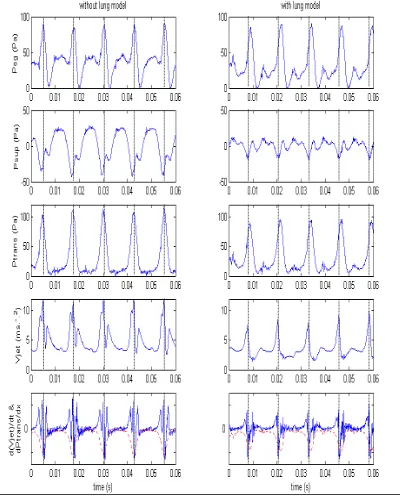
Figure 4 shows simultaneous time histories for 5 shutter cycles of i) pressure 30 mm upstream of the glottal exit (Psg), ii) pressure 50 mm downstream of the glottal exit (Psup), iii) transglottal pressure Ptrans (= Psg – Psup), iv) velocity for x = 0, at 5 mm downstream of the glottal exit (Vjet) and v) the time differential of Vjet (solid line) and the spatial derivative of − Ptrans (dotted line). For Psg, the steady upstream pressure has been added to the time history. The left-hand graphs correspond to CVFR and the right-hand graphs to CP. The volume flow rate at the rotameter was 200 cm3 s-1 in both case.

For Psg, the peak pressure amplitude remains unchanged when the lung model is added, but while for CVFR the pressure increases sharply after glottal opening and then remains relatively steady until the next closure, for CP a sharp recovery on opening is followed by a further smaller dip before the increase associated with the narrowing glottis. For CP, the large peak in Psg is delayed with respect to glottal closure by approximately 11% of a cycle as compared to a delay of approximately 3% of a cycle for CVFR. In both cases the mean pressure is lower than would be expected in vivo, and this is consistent with the short closure time in the model as compared to that typical of male modal voice.

During glottal closure, Psup shows a trough, which is significantly deeper for CVFR than for CP. This is followed by a pressure recovery during opening that is again larger for CVFR. In both cases, from about 3 ms before until 3 ms after maximum glottal opening there is a strong resemblance between the shape of Psg and Psup suggesting coupling between the sections of the duct upstream and downstream of the glottis.

The trans-glottal pressure difference, Ptrans, shows a large peak at glottal closure, which occurs somewhat later for CP than for CVFR due to the delay in Psg already described. The peak for CP shows a 17% reduction in amplitude compared to CVFR, which corresponds reasonably well to the observed reduction in amplitude in Vjet (24%). Better agreement might be expected if Psg and Psup had been measured at positions closer to the glottal exit; adjustments to the model to allow this will be made in future. Between the peaks, Ptrans is relatively constant for CVFR but shows a small increase and decrease for CP.

The features described previously for Vjet can clearly be seen in the graphs. In addition one can observe that the peak on opening for CVFR is in temporal registration with a notch in Psup. No corresponding feature can be observed in Psg. For CP the smaller, delayed opening peak is in temporal registration with small peaks in both Psup and Psg.

−dPtrans/dx. Again, a better agreement might be expect if Psg and Psup were to be measured nearer the glottal exit. For a volume source model of sound generation at the glottal exit, the source strength will vary with dVjet/dt and thus the larger variation for CVFR suggests that this configuration will be associated with a stronger acoustic excitation of the duct. Experiments to investigate sound generation in each case are in progress.

Figure 4: Time histories of (top to bottom): upstream pressure (Psg), downstream pressure (Psup), transglottal pressure (Ptrans), jet velocity at x = 0, 5 mm from glottal exit (Vjet) and (on the same axes) time differential of Vjet (solid) and spatial differential of

DISCUSSION

The graphs of Figure 4 show some distinct changes to the upstream and downstream pressure time-histories and to the glottal jet time-history when the lung model is in position. These changes affect the waveform shape, the timing and existence of features within the waveforms and, for the measurements downstream of the glottis, the amplitude.

The upstream compliance included for CP presents a more realistic geometry for the model. It is not, however, possible to say definitively that it therefore produces more realistic waveforms for the pressure and velocity downstream of the glottis.

Direct comparison of the pressure time-histories with in vivo measurements such as those of Cranen and Boves (1985) is problematic due to the short closure time in the model glottis as compared to the closure time of the order of 50% of a glottal cycle that they encountered. With its uniform, unconstricted duct, the model should be best approximated by their in vivo measurements for /a/. However, for this vowel one observes an oscillation in the pressure time-history due to formant excitation after glottal closure in vivo, which is not observed in the model measurements.

Qualitatively, the supra-glottal pressure measurements of Cranen and Boves for /a/ are perhaps more like the CP case than the CVFR case due to the relatively smaller positive pressure during opening. A much larger negative pressure is observed in vivo during closure than is found for either CP or CVFR. For Psg, the in vivo measurements show similarities to both CP and CVFR, with neither in vitro case being noticeably a better approximation.

It is, however, clear from the observations presented here that when interpreting measurements from dynamic mechanical models, researchers should be aware that the upstream duct geometry can have an effect on the pressure and velocity time-histories, which will need to be considered carefully when discussing details of waveform shape and relative timing.

ACKNOWLEDGEMENTS

This work was support by an EPSRC Fast Stream award no. GR/M99200. Thanks are due to Dr A Hirschberg of TU Eindhoven NL for suggesting the importance of the upstream geometry.

REFERENCES

Alipour, F. and Scherer R. C. Effects of oscillation of a mechanical hemilarynx model on mean transglottal pressures and flow, J. Acoust. Soc. Am., 110, 1562-1569 (2001).

Barney, A., Shadle, C.H. and Davies, P.O.A.L., Fluid flow in a dynamic mechanical model of the vocal folds and tract: Part I Measurements and theory, J. Acoust. Soc. Am., 105, 444-445 (1999).

Cranen, B. and Boves, L. Pressure measurements during speech production using semiconductor miniature pressure transducers: Impact on models for speech production. J.Acoustic. Soc. Am., 77, 1543-1551, (1985).