COMPARATIVE STUDY OF VARIOUS TECHNIQUES TO MEASURE SPEECH INTELLIGIBILITY

COMPARATIVE STUDY OF VARIOUS TECHNIQUES TO MEASURE

SPEECH INTELLIGIBILITY

PACS REFERENCE: 43.55.Hy

Galindo, Miguel; Zamarreño, Teófilo; Girón, Sara

Dep. of Applied Physics II; High School of Architecture; Seville University Avda. Reina Mercedes, 2

41012 - Seville Spain

Tel.: +34 954556612 Fax: +34 954557892 E-mail: teofilo@us.es

ABSTRACT

The aim of this paper is to compare two different methods of measuring the Modulation Transfer Functions (MTF) and the corresponding derived STI-RASTI indices to assessing intelligibility. The first method uses, as test signal, a band filtered (500 and 2000 Hz) amplitude modulated noise. The second one uses MLS signals to obtain the impulse response of the system; further post processing allows us to calculate the MTF and STI-RASTI indices from this filtered response.

INTRODUCTION

The Speech Transmission Index (STI) and the Rapid Speech Transmission Index (RASTI) were proposed by Houtgast and Steeneken [1]-[3] to evaluate speech intelligibility, where RASTI is a reduced version of STI. Both are calculated from the Modulation Transfer Function (MTF) defined as the ratio of modulation amplitude intensity of the perceived signal by that of the emitted one:

( )

m

m F

m

=

The m(F) values are obtained for each modulation frequency F between 0.63 Hz and 12 Hz in 1/3 octave steps (14 in total). This range covers the speech modulations. The carrier noise signal is octave band filtered between 125 Hz and 8 kHz. In this way there are 7×14=98 m(F)

values. These modulation reduction factors are converted into apparent signal/noise ratios and are properly weighted and averaged to calculate the STI index [3]. Fig.1 shows a possible scheme to calculate MTF. This method is implemented, for example, in the free PC-software STI ver.-2.0 from Lexington School for the Deaf [4], where the stimulus signal consists of a band limited white carrier noise modulated by low frequency sine waves. Each measure takes about 2 minutes to apply all the modulation frequencies to the test system successively.

Schroeder [7] proposed an alternative method to the scheme of Fig. 1 to find the m(F) values for linear, passive and time invariant systems from the impulse response h(t). In this case, it’s necessary to filter h(t) for each octave band of the carrier, f. The m(F) values are calculated from the filtered impulse response hf (t) according to:

2

0

2

0

( )·exp(

2

)

( )

( )

f

h

j

F

d

m F

h

d

τ

π τ τ

τ τ

∞

−

=

∫

∫

The impulse response can be obtained using an impulsive signal (shot), but in this case we cannot take into account the background noise because the spectrum of the impulsive signal is very different from the normalized speech spectrum defined by Houtgast and Steneken [1]-[3], or even those proposed by IEC [8]. In table 1 we show the normalized values to the speech reference spectrum at 250 Hz.

This difficulty can be overcome using Maximum Length Sequences (MLS) as stimulus signal in order to obtain the impulse response, as Rife pointed out [9]. In this case it’s possible to insert a filter between the MLS generator and the input of the amplifier to adapt its spectrum. Table 1 also shows the filter transfer function normalized to the value at 250 Hz octave band and is compared with the reference speech spectrum in Fig. 2.

In order to obtain reliable MTF measures, in addition to general requirements for measures with MLS signals, we must keep in mind some considerations, such as:

• Measuring an impulse response long enough (at least 1 s) with a minimum bandwidth of 12 kHz (3 kHz for RASTI measurements).

• Not averaging to obtain the impulse response. This will artificially reduce the signal/noise ratio (the S/R increase +3 dB every time the number of MLS periods are doubled). Even though it’s possible to take advantage from this situation to evaluate the incidence of background noise against other modulation degradation factors.

Table1.- IEC speech spectrums and filter transfer function used for the MLS measures. Octave Ref. spectrum Male voice Female voice Measured filter

125 -2,5 2,9 -200,0 -0,55

250 0,0 2,9 5,3 0,00

500 -1,0 -0,8 -1,9 -1,43

1000 -5,0 -6,8 -9,1 -4,60

2000 -10,0 -12,8 -15,8 -9,52

4000 -17,0 -18,8 -16,7 -16,80

8000 -23,0 -24,8 -18,0 -25,30

Frequency (Hz)

125 250 500 1000 2000 4000 8000

Attenuation (dB)

-30 -25 -20 -15 -10 -5 0 5

Reference speech Adapter filter

Fig 2.- Reference speech spectrum and filter transfer function.

System under test

Stimulus signal: Response signal

x2 _x2

1₂ (carrier) (1 sin(2 _m))

Noise × + πF t

system noise & distortion]

 

+ 

 

 

emi

m

per

m

• Reproducing the MLS signal by an acoustic source with the same directivity as the human head has, if there isn’t an electroacoustic system. If it exists, the signal will be applied to the audience by the loudspeakers of the system.

• Reducing the bandwidth to avoid time aliasing errors when the reverberation time is too long (about 7 s in our system). Dividing by two, the bandwidth allows us to double the reverberation time for reliable measures (although this implies that the high frequency bands are not computed to calculate the STI).

EXPERIMENTAL RESULTS AND DISCUSSION

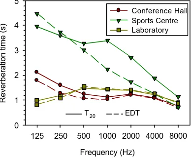
We present here the measured data for three different rooms, which are in the High School of Architecture: the Physics Laboratory, the Conference Hall and the Sports Centre. Their approximate volumes are 320, 1870 and more than 9300 m3 respectively (see Fig. 3). Their reverberation times (T20 and EDT) for the octave bands between 125 and 8000 Hz were

measured using MLS technique through the analyser based in PC MLSSA from DRA laboratories [10]. For each measure we average eight MLS periods in order to improve the S/N ratio. The signal was acquired by the omnidirectional microphone B&K-4269. These results appear in fig. 4.

To evaluate the speech intelligibility we have measured STI/RASTI indices using two different systems: (i) the Brüel & Kjær Speech Transmission Meter type-3361 uses the modulated noise technique. The emission level was adjusted to Ref+10 dB; this implies a SPL of 69 dB at the 500 Hz octave band and 60 dB at 2 kHz,

measured at 1 m from the source (≅67 dB(A)). The duration of each measure is set up to 16 s. We have been using this technique for several years with good results [11]. (ii) The MLSSA analyser uses the MLS technique. The spectrum envelope of this signal is described by sin2(x)/x2. The sampling frequency is adjusted by MLSSA to three times the demanded bandwidth, so that in that condition the spectrum is practically flat. For this reason the MLS signal is conditioned by the filter CWF-1 from One to One Technical Products before entering the amplifier input. The filter transfer function was measured using MLSSA and is

displayed in Fig. 2. The amplified signal is Frequency (Hz)

125 250 500 1000 2000 4000 8000

Reverberation time (s)

0 1 2 3 4 5

T₂₀ EDT

Conference Hall Sports Centre Laboratory

Fig. 4.- Measured reverberation times. Laboratory Conference Hall

Sports Centre

delivered to the audience by two different sources, a dodecahedral source B&K-4296 and a reference acoustic source B&K-4205. The signal was adjusted, following manufacturer’s recommendations, to produce a sound pressure level of 67 dB(A) at a source-microphone distance of 1m. This level was checked by the sound level meter B&K-2231. In all cases the emitter was located at the position marked S in Fig. 3.

The signal was captured using two different omnidirectional microphones: the B&K-4190, calibrated before measuring, and the AT4050/CM5 from Audio-Technica, which was unable to be calibrated. Each one of them with their respective preamplifier and polarization source (B&K-2804 for the first case and LAB1 from Earthworks for the second one). In order to evaluate the effect of background noise we made calibrated measures, without averaging, and uncalibrated measures, averaging eight MLS periods, to obtain h(t). To calculate STI values it’s possible to choose among three different spectrums: reference one, men spectrum or women spectrum from IEC-268-16 [8]. The values we have used in this paper correspond to reference spectrum.

Fig. 5 shows RASTI values measured in order to evaluate the fluctuations caused by small imprecisions in the placement of the microphone. Measurements were performed both with the B&K (modulated noise) and MLSSA analyser (MLS signal), for a fixed microphone position (P-5 in laboratory) and moving the microphone around this position. The blue lines correspond to the 95% confidence interval (±0.02) that we can take as random errors. As we can see, there are no meaningful differences for either the two measurement techniques or for the microphone positions. The background noise for the measurement time was stationary and lower than 35 dB(A).

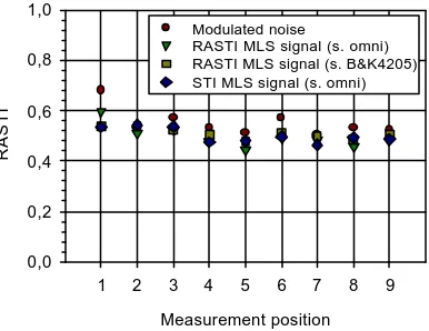
Measurements for all positions in the laboratory with the two mentioned sources have been carried out (Fig. 6). Some minor differences appear between the values measured with different techniques (even between RASTI and STI measured with MLSSA). The background noise was similar to the previous situation. Meaningful dispersions for the two sources do not appear. These differences are only noticeable when the microphone is located laterally from the source due to the voice directivity (see P-1, P-3 in Fig. 8).

In order to dispose of a greater interval of STI/RASTI values, we have repeated these measurements with increasing wideband stationary background noise levels produced by the reference acoustic source Brüel & Kjær type 4205 (Fig. 7). In this situation the RASTI and STI values measured with MLSSA appear different. We could expect this result since RASTI only computes the effects for 500 and 2000 Hz octave bands, while STI is affected from wideband noise spectrum. The differences between RASTI values from B&K-3361 and those calculated from impulse response measured with MLSSA are strongly dependent on the noise level. The mayor differences appear (Fig. 7(b)) when the noise level is similar to the signal level, 64dB(A). Similar results are obtained in the Conference Hall (Fig. 8), measured with HVAC off (low and stationary noise level: Leq=36 dB(A); L10=37 dB(A) and L90=35.5 dB(A)) and the HVAC on. In

this case the background noise effect can be observed at positions around the grid (12-16) (the measured noise levels at point 16 are Leq=49.8 dB(A); L10=50.5 dB(A) and L90=49.5 dB(A)). The

Number of measure

1 2 3 4 5 6 7 8 9 10 11 12

RASTI

0,0 0,2 0,4 0,6 0,8 1,0

B&K-3361 fixed B&K-3361 not fixed MLSSA (RASTI) fixed MLSSA (RASTI) not fixed 95% confidence

Fig. 5.- Measured RASTI values at P-5 (laboratory) with the microphone at fixed pos ition (“fixed”) and

moving it around (“not fixed”).

Measurement position 1 2 3 4 5 6 7 8 9

RASTI

0,0 0,2 0,4 0,6 0,8 1,0

Modulated noise

RASTI MLS signal (s. omni) RASTI MLS signal (s. B&K4205) STI MLS signal (s. omni)

differences are more noticeable for the results from the Sports Centre (Fig. 9), where the traffic noise level is higher and, above all, time-variant (Leq=47 dB(A); L10=50 dB(A) and L90=42 dB(A)).

If background noise is negligible and the reverberation effect is the main reason for the loss of intelligibility, then STI values derived from uncalibrated MLS signals (averaging several MLS cycles in order to obtain impulse response) are similar to that obtained from calibrated ones (without averaging) (Fig. 8, HVAC off).

We have also compared the results obtained from two very different microphones with MLSSA. The results are very similar (Fig. 10). The reason for this comparison is that Audio-Technica is a multipattern microphone which can be used to measure other acoustic parameters (LF, LFC) simply selecting between omnidirectional and figure eight pattern.

(a) Measurement position

1 2 3 4 5 6 7 8 9

STI / RASTI

0,0 0,2 0,4 0,6 0,8 1,0

Modulated noise RASTI MLS signal STI MLS signal

(b) Measurement position

1 2 3 4 5 6 7 8 9

STI / RASTI

0,0 0,2 0,4 0,6 0,8 1,0

(c) Measurement position

1 2 3 4 5 6 7 8 9

STI / RASTI

0,0 0,2 0,4 0,6 0,8 1,0

(d) Measurement position

1 2 3 4 5 6 7 8 9

STI / RASTI

0,0 0,2 0,4 0,6 0,8 1,0

Fig. 7.- Measured RASTI / STI values with different wideband background noise levels: (a) 54 dB(A), (b) 64 dB(A), (c) 74 dB(A) and (d) 80 dB(A); all of them measured at 1m from noise source.

Measurement position

2 4 6 8 10 12 14 16 18 20 22

RASTI

0,0 0,2 0,4 0,6 0,8 1,0

Calibrated MLS signal (HVAC off)

Calibrated MLS signal (HVAC on) Uncalibrated MLS signal (HVAC off)

Fig. 8.- RASTI values for the Conference Hall measured averaging 8 cycles MLS signal and

without averaging (HVAC on and off).

Measurement position

2 4 6 8 10 12 14 16 18 20 22

STI / RASTI

0,0 0,2 0,4 0,6 0,8 1,0

Modulated noise MLS signal (RASTI) MLS signal (STI)

Finally, Fig. 9 represents the correlation between all measured data using the B&K and the MLSSA analyser with the 95% prediction interval. In it, we have marked the qualification intervals: green for “bad” , pink for “poor”, cyan for “fair”, blue for “good” and red for “excellent”. We can see how the qualification derived from MLSSA values can be different (and lower) from those derived from B&K values mainly in the “poor” interval. It would be necessary to make more measurements to obtain more values in the range good and excellent.

CONCLUSIONS

We have compared two different techniques for measuring speech intelligibility. We have observed a minor influence of the microphone and of the loudspeaker in the MLS technique. However, the presence of background noise supplies values that differ from those measured with noise modulated technique and, above all, if the background noise is of the same order of the test signal or time-variant. Probably in this situation the condition of time-invariant it’s not fulfilled by the room and consequently the intelligibility qualification can differ according to the technique used. We haven’t carried out the analysis of the measured MTF due to space reasons.

REFERENCES

[1] Steeneken H.J.M. and Hougast T., The modulation transfer function in room acoustics as a p redictor of speech intelligibility, Acustica 28, 66-73, 1973.

[2] Hougast T. and Steeneken H.J.M., A multi-language evaluation of the RASTI-method for estimating speech intelligibility in auditoria, Acustica 54, 185-199, 1984.

[3] Hougast T. and Steeneken H. J. M., A review of the MTF concept in room acoustics and it’s use for estimating speech intelligibility in auditoria, J. Acoust. Soc. Am. 67, 1060-1077, 1985.

[4] http://hearingresearch.org/STI.htm

[5] Speech transmission meter type 336. Reference manual. Brüel&Kjær, Nærum, Denmark. [6] http://www.bruel-ac.com (E-mail: bruel@mclink.it)

[7] Schroeder M. R., Modulation transfer function: definition and measurement, Acustica 49, 179-182, 1981.

[8] Redraft of IEC 268-16, sound system equipment, part 16: The objective rating of speech intelligibility by the speech transmission index.

[9] Rife D., Modulation transfer measurement with maximum length sequences, Journal of the Audio Engineering Society 40 (10), 779-790, 1992.

[10] MLSSA, Maximum-length sequence system analyser, reference manual, v. -10W. DRA laboratories. [11] Galindo M., Zamarreño T., Girón S., Speech intelligibility in Mudejar-Gothic churches. ACUSTICA

Acta Acustica 86, 381-384, 2000.

RASTI B&K

0,0 0,1 0,2 0,3 0,4 0,5 0,6 0,7 0,8 0,9 1,0

RASTI MLSSA

0,0 0,1 0,2 0,3 0,4 0,5 0,6 0,7 0,8 0,9 1,0

y = 1,061*x - 0,0986 r2 _{= 0,883}

Fig. 11.- Correlation between different techniques RASTI measured values in the three rooms. Measurement position

2 4 6 8 10 12 14 16 18 20 22

STI

0,0 0,2 0,4 0,6 0,8 1,0

Microphone Brüel & Kjaer Microphone Audio-Technica

Fi g. 10.- STI values measured with two different