72 MODELS AND ALGORITHMS FOR COMPUTER SIMULATIONS IN ROOM ACOUSTICS

MODELS AND ALGORITHMS FOR

COMPUTER SIMULATIONS IN ROOM ACOUSTICS

Reference PACS: 43.55.Ka

Vorländer, Michael

Institute of Technical Acoustics - RWTH Aachen University Neustr. 50, 52066 Aachen, GERMANY

mvo@akustik.rwth-aachen.de

ABSTRACT

With the rapid development of computers, commercial software for room acoustical simulation is available. It is only complete with an option for auralization. Another field of rapid progress is Virtual Reality. In this contribution the development of simulation tools in room acoustics and further work aiming at real-time Acoustic Virtual Reality systems are reviewed and discussed with particular emphasis on the level of detail in CAD models, on curved surfaces, on diffraction, on stochastic uncertainties in input data, on small rooms, and on real-time processing.

1. INTRODUCTION

With the rapid development of computers, room acoustical simulation software was developed and applied in sound field analysis in rooms. Finally in the beginning of the 1990’s, the pro- cessor speed, the memory space and the convolution machines were sufficiently powerful to allow room acoustical computer simulation and auralization on a standard personal computer. Since then, several improvements in the modelling algorithms, in binaural processing and in reproduction techniques were made (see Kleiner et al [1]). Commercial software for room acoustical simulation today is only complete with an option for auralization through the sound card of the computer.

The concept of auralization was applied to fields other than room acoustics since about the year 2000. The aim is now different as not music and the quality of concert halls or other performance spaces are to be evaluated but the perception of sound and noise. Thus, building acoustics, automotive acoustics and machinery noise are areas of application. The task in all these applications is the evaluation of sound sources, transmission constructions or products by listening instead of a numeric expression of the acoustic quality [2]. Wave-based numerical acoustics such as FEM, BEM, FDTD or analytic models and any kind of structural acoustics transfer path method is suited as a basis for auralization. The link between simulation and auralization is the representation of the problem in the signal domain and the treatment of sound and vibration by signal processing [3].

Another field of rapid progress is Virtual Reality. Originally used in computer graphics and visualization, Virtual Reality aims at image simulation (so-called “rendering”) and 3D displays. In this contribution the development of simulation tools, examples for applications in room acoustics and further work aiming at real-time Acoustic Virtual Reality systems is reviewed and discussed.

of auralization by separation of the processes of sound generation and transmission into system blocks and description of these blocks with tools of system theory. Fig. 1 illustrates the basic elements of sound generation, transmission and radiation.

Figure 1. Components of auralization and virtual acoustics: representation of sound and vibration sources, transmission, reproduction, and mapping on a task of signal processing.

One might ask why the problem cannot simply be treated by using a mono signal, an equalizer and a headphone. The need for a more complex reproduction technique with a spatial representation is given by the fact that human hearing extracts information about the sound event and the sound environment by segregation of acoustic objects due to common cues of spectral, temporal and spatial attributes. This, for instance allows us to identify one speaker out of a cloud of diffuse speech (cocktail party effect). In situations of noise immission, the spectral, temporal and spatial cues are extracted to judge the event as pleasant, annoying, informative or neutral. As long as the specific acoustic (physical) and semantic content of the noise must be treated, restrictions in spectral, temporal and spatial cues are not appropriate.

In room acoustics, the quality of the results must be very high. People are sensitive to the perception of music in all its aspects, temporal, spectral and spatial. Therefore the challenge in creating auralization in room acoustics is very high, and this applies to source recording, sound propagation (reverberation) rendering and audio reproduction. While source recording and audio reproduction is discussed in other papers, this contribution is focused on simulation of the sound propagation in rooms.

2. ROOM ACOUSTICAL SIMULATION

Today, simulated room acoustics are applied in various fields with great success. Their well- developed algorithms help to create realistic acoustics during architectural planning. Acoustic simulation tools are also used for designing sound reinforcement systems in churches, stadiums, train stations and airport terminals.

2.1 Geometrical acoustics: Ray Tracing and Image Sources

In geometrical acoustics the two basic models of geometrical sound propagation, ray tracing and image sources are applied. Often, however, the two philosophies are mixed up, even confused. It is important to highlight the differences in the physical meaning: Ray tracing describes a stochastic process of particle radiation and detection. Image sources are geometrically constructed sources which correspond to specular paths of sound rays. Often, image sources are constructed by using rays, beams or cones, via kind of ray tracing.

image sources and ray tracing is the way of calculation of contributions in impulse responses. Ray Tracing only yields impulse response low-resolution data like envelopes in spectral and time domains. Image sources (classical or via tracing rays, beams, cones, etc. [4 - 8]) may be used for exact construction of amplitude and delay of reflections which narrow-band resolution depending on the filter specifications for wall reflection factors, for instance.

2.2 Hybrid models

Due to the contradictory advantages and disadvantages of ray tracing and image sources it was tried to combine the advantages in order to achieve high-precision results without spending too much complexity or computation time. Either ray tracing or radiosity algorithms were used to overcome the extremely high calculation time inherent in the image source model for simulation of the late part of the impulse response (adding a reverberation tail), or ray tracing was used to detect audible image sources in a kind of “forward audibility test”. The idea behind is that a ray, beam, or cone detected by a receiver can be associated with an audible image source. The order, the indices and the position of this image source can be reconstructed from the ray's history with storing the walls hit and the total free path. Hence the total travel time, the direction and the chain of image sources involved can be addressed to the image source. Almost all other algorithms used in commercial software are kind of dialects of the algorithms described above, and they differ in the way mixing of the specular with the scattered component is implemented. The specific choice of dialect depends on the type of results, particularly on the accuracy, spatial and temporal resolution.

2.3 Verification tests

The computational performance and the accuracy of computer simulations can only be checked if existing rooms are modelled and the results compared with measurement results. Auralization, of course, can also be checked in listening tests with recordings in the original room. This procedure was carried out in a first intercomparison in Braunschweig in 1993 and 1994, Germany, on a lecture hall. The first results were partly disappointing [9]. Data were collected from 17 participants in computer simulations and 7 in measurements. One result is shown in Figure 2. It contains the prediction of reverberation time based on visual inspection of the test room and individual choice of absorption coefficients. The results of this phase showed a surprisingly large scatter with a strong tendency to underestimate the absorption coefficients and thus to overestimate the reverberation time.

Figure 2. Results from the first round robin on room acoustical computer simulations (from [9]). Plot of reverberation times T predicted for the 1 kHz octave band in an auditorium. Thick line: average

measurement result which has an uncertainty of 5% (± 0.05 s) ([10]).

however, only a few programs were identified reliable. Moreover, it was significant that algorithms with purely specular reflection modelling are not sufficient which was supported by the results of the second phase where the input data were fixed for all participants. Still the programs which only used specular reflections overestimated the reverberation time systematically. Today it is common knowledge that in typical rooms after reflection order three or four, the main energy propagation goes through diffuse (scattered) sound.

In the following years, two more round robins were created by Bork in 2000 [9] and in 2005 [10]). He confirmed the results of the first project and who extended the scope and the interpretation towards new aspects.

3. CAUSES AND CONSEQUENCES OF UNCERTAINTIES

In the following we investigate the sources of uncertainties and their impact on the results. In this discussion, an uncertainty must be treated as object of scientific research on its own. It is not adequate to “calibrate” a computer model with adjustment of input data in a way that, for instance, reverberation times or other damping effects are matched to measurement results. The objective for computer simulation should be to be independent of adjustment factors. It should be purely based on physical data and corresponding databases of input data (typically material properties).

If correct data are used, there still remains the question of the correct model and the correct method suitable for solving the acoustic problem. The latter aspect sets demands on the skills and experience of the operator. For this paper, we assume that the operator uses the software under appropriate conditions of applicability to the acoustic problem. Then remain systematic and stochastic errors due to the algorithm itself.

In the analysis of stochastic uncertainties, a very powerful tool can be applied which is related to uncertainties of measurements (ISO GUM). The principles suggested in this “ISO Guide to the expression of uncertainty in measurement” have not yet been considered in acoustics in a wide sense. And in computational acoustics there is hardly a systematic approach to tackle the problem of uncertainties with a comparable insight which is available for some acoustic measurements (typically high-precision calibration techniques where uncertainties must be stated as part of the result).

It is sensible to define a scale of psychoacoustic relevance of differences and, thus, comparing differences between results or quantitative uncertainties addressed to simulations with the just audible differences (JND) of human hearing. In best case of listening environment in the laboratory by using headphones, for instance, the JND for reverberation time is about 5%, for strength (level) 1 dB and for definition 10% (after [9]). If uncertainties are smaller than these values, the simulation can be considered as sufficiently precise. For computer prediction and simulation including auralization, one could state the general rule of “don’t compute what you can’t hear”. This statement, however, is quite useless in other applications such as in discussing uncertainties in calibrations, for example.

3.1 Level of detail

The reasons for deviations between simulations and measurements are shortcomings in the algorithms and the modelling approach behind it. As described before, ray tracing (or similar) and the image model are the basis for all simulations. In the following, some examples are discussed in which the physics of wave propagation is only too roughly approximated. Errors may possibly occur, and it is the question if these affect parameters like reverberation time or clarity, or if the approximations are audible.

unnecessary long computation times. Accordingly a large potential is identified in the acceleration of algorithms at low frequencies at low spatial resolution in the CAD model, and at late times in the impulse response, where the late decay is built by scattering rather than by deterministic specular reflections in a detailed CAD model. In an ongoing project it is inverstigated which criteria can be used for choosing appropriate level of detail in CAD models [13] (see Figure 3). These findings will be also relevant for simulation large volumes such as cathedrals, stadiums, airports and trains stations at reasonable computation times.

Figure 3. Level of detail in a CAD model of a concert hall illustrated for (top to bottom) low, mid and high frequencies (after [13]).

3.2 Curved surfaces

To the author’s knowledge, none of the simulations packages allows modelling of curved surfaces. Usually curved surfaces are approximated by a number of planes. Curved surfaces produce very special features like focal points or caustics. The questions is if an approximation by planes produces a focus as well and if the sound level in the focal region is correct ([15, 16]) It was shown that only deterministic approaches with coherent image source contributions can be used.

Low

α (

≈

0.1)

0.1

Mid

α (

≈

0.4)

0.1

High

α (

≈

_0.9)

0.2

extremely high pressure by absorbers or diffusers in the curved boundary is not enough to eliminate the focussing effect. Outside the focal a strong interfering sound field is observed. Vercammen concludes that within reasonable accuracy the sound field outside the focus can be calculated with geometrical acoustics. But computer models based on image source methods are not capable of describing the focal pressure.

3.3 Diffraction

Diffraction in room acoustics mainly happens for two reasons: There can be obstacles in the room space (e.g. stage reflectors), or there can be edges at surroundings of finite room boundaries. In the latter case, either the boundary is forming an obstacle, such as columns or the edge of an orchestra pit, or the boundary is forming the edge between different materials with different impedances (and absorption). Since diffraction is a typical wave phenomenon, it is not accounted for by the basic simulation algorithms listed above. In the past there were some ideas of including diffraction as a statistical feature into ray models. But the success was quite limited because the increase in calculation time is a severe problem. In optics and radiowave physics, ray tracing models were generalised into so-called UDT (uniform geometrical diffraction theory [19]). Other approaches were presented by Svensson [20], who applied the model by Biot and Tolstoy [21] and by Stephenson [22]. They are very powerful for determination first-order diffraction. All methods of geometrical diffraction are, however, very time consuming for simulation of a multiple-order diffraction and corresponding reverberation.

Most recently, Svensson and Schröder implemented diffraction modules in simulation software for both stochastic ray tracing and deterministic image sources [23, 24]. Tests and comparions with experiments are subject to ongoing work. Therefore, in all cases where room modes are to be calculated, in small studio rooms, in living rooms or in other examples, only wave-based models can be used, such as BEM or FEM or similar.

3.4 Stochastic uncertainties in input data

Source of stochastic uncertainties in simulations are usually introduced by uncertain input data, mainly by boundary conditions of absorption and scattering. These data are often taken from databases or textbooks, or they are integrated databases in software.

The stochastic uncertainties are caused by influences of the operator and by uncertainties of material properties, either in uncertainties of the product specification from standard measurements or by manufacturing variations of the products. In the following we exclude influences of the operator, since this component is not predictable. Also, the model of the geometry, the “polygon model”, is for the moment considered as perfect. For constructing polygon models in geometrical acoustics similar guidelines exist, such as “walls-large-compared-with-wavelength”. For the following we neglect these uncertainties. Also neglected are uncertainties from too low computation time due to an insufficiently low number of rays, low reflection order etc. We now only consider material input data.

For geometrical acoustics there exist a few preliminary studies of the influence of material data on the prediction results. In contrast to data of complex impedances or reflection factors, tables of absorption coefficients are widely available in textbooks and online. The question concerning simulation software is here focused on the implementation. Should α be modeled angle-dependent or just be constant (random incidence)?

ISO 354 provides a standard method for measuring random-incidence absorption coefficients in reverberation rooms. The uncertainty inherent in the method can be expressed as follows:

Table 1. Uncertainty of absorption coefficients (ISO 354)

Surface scattering occurs if wall surfaces are corrugated. The specific reflection pattern depends strongly on the frequency. However, with diffuse field conditions and the corresponding uniform sound incidence, not the detailed reflection characteristic is needed, but knowledge about a random-incidence scattering coefficients, which is defined as the ratio between the scattered sound energy and the totally reflected sound energy [25]. There are no tables available in depth, except one first attempt in [3]. And also here: Should scattering be implemented in the software with angle dependence or just for the random-incidence average?.

The question of angle dependence cannot be solved generally. If the sound field provides a good mixing and, thus, a good diffuse field approximation, the random-incidence data are surely sufficient. In non-mixing geometries such as corridors or flat halls, this effect may not be taken as granted, and instead of the average, specific angles of incidence dominate the losses. For scattering walls it can be expected that differences are noticeable for vertical or horizontal orientation of 1D structures [26].

4. SMALL ROOMS

For acoustic rendering of car compartments geometrical acoustics is not sufficient. Wave-based models must be used as well, because relevant parts of the frequency response are below the Schroeder frequency. In this example, a combination of FEM (with subsequent inverse FFT) and geometrical acoustics is applied. At the crossover frequency the two transfer function are linked in a very similar way as used in loudspeaker crossover networks.

Figure 4. Simulation package for small room acoustics (after Aretz [27]).

With extensive measurements and modelling of the acoustic characteristics of the car materials a good agreement between measured and simulated results was achieved. However, as Aretz [26] clearly points out, further investigations regarding the boundary and source representation and diffraction are necessary to improve the simulation accuracy, see also [28].

5. REAL-TIME SIGNAL PROCESSING

instance, when a person is leaving a room and closing a door, require complex models of room acoustics and sound insulation. Otherwise the coloration, the loudness and timbre of sound within and between the rooms will not be sufficiently represented. Another example is the interactive movement of a sound source behind a barrier or inside an opening of a structure so that the object is no longer visible but can be touched and heard (by diffraction). The task of producing a realistic acoustic perception, localization and identification is a big challenge [29, 30].

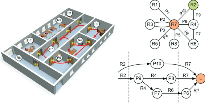
Real-time processing requires dramatic reduction of complexity on several levels. At first, the model geometry must be kept as simple as possible but also as accurate as possible. Therefore not only the physical but the psychoacoustic evaluation is important as well to evaluate the degree of complexity necessary. If this problem is to be solved, the data handling concerning scene and object management must be very efficient. Finally, the filter representing the sound and vibration trans-mission system is the basis for convolution of the source signal of choice. Usually we talk about a dry source signal (recording), but generally it can be also a force or vibration source signal, as described above. In the following, data management and convolution problems are briefly discussed in the light of real-time performance.

Figure 5. An example of an office building and the corresponding acoustical scene graph describing the topological structure of a room acoustic scene and acoustic coupling of interconnected rooms via portals

(after Wefers and Schröder [31]), see also Fig. 6.

5.1 Data management

Imagine a ray tracing algorithm and a scene with many (more than 100) polygons, where the actual ray intersection point with the right wall polygon must be found (the same by the way is a task in image source models). In a brute-force approach the polygons are listed in serial order, and on average half the list must be checked until the right candidate is found. This is far too slow. Therefore in acoustic ray tracing as well as in computer graphics methods for speed-up were developed, and these consist of clever data structures for fast search algorithms.

5.2 Fast convolution

For rendering of complex scenes, a partitioned fast convolution must be created. The general principle of such an algorithm for one channel consists of two main parts: Stream processing and filter processing. The algorithm can be split into four major parts:

1. Packing and FFT transformation of the input data (source signal) 2. Packing and FFT transformation of the filter data (transmission system) 3. Spectral convolution (complex-valued multiplication and accumulation 4. IFFT transformation and unpacking of the output data

Now, it is crucial how this kind of block processing is organized. With large blocks the gain of processing speed due to FFT algorithms is large, but the large block requires the time of the block length to be loaded into the convolution buffer. This is simply due to the running (continuous) audio stream from the source file. This waiting time to feed the block with data causes “latency”, a very important effect in real-time systems. It simply means that the output has a delay related to the input. The critical range is already found at several ten milliseconds. Imagine the user knocking a virtual door and the knocking sound does not coincide with the visual and haptic perception.

Figure 6. An example of the filter chain for acoustical scene graph for the topological structure described in Fig. 5 (after Wefers and Schröder [31]).

The processing time for interaction is relevant as well. Partly special processors and filter partitioning were used to speed up the convolution ([32, 33]). In dynamic situations the user can freely move. Other receiving points may require new transmission system filters. The filters must be changed without fading arte-facts. The key methods to achieve real-time performance are grouping of signal transmission paths and connecting through portals. The subsystems are characterized by their impulse responses between source, receivers and interfaces. Interfaces such as portals typically have insulating properties which can be modelled by simple equalizers effects. Binaural processing is only required in the last filter for modelling the listener.

6. CONCLUSIONS

After some decades of development in room acoustics simulation, progress was made indeed. This fact is related to the results of the “round robins” and on success in numerous applications for room acoustics design. User guides, however, are still uncertain and they do not generally provide a good basis for using any software. Software specifications differ particularly in the transition of early / late response modelling, and in treatment and combination of both specular and diffuse reflections. As long as the user is not sure how many rays shall be chosen, how the resolution of the geometrical CAD model is to be defined, how the scattering coefficients are found and the transitions order between early and late parts is chosen, uncertain results may occur. It is not, however, a task of research to find out those differences, it should be a clear user guideline for each simulation software applied.

7. REFERENCES

[1] M. Kleiner et al., “Auralization – an overview”, J. Audio Eng. Soc. 41, 861 (1993)

[2] M. Vorländer, “Engineering Acoustics meets Annoyance Evaluation”, Proc. Internoise 2005, Rio de Janeiro (2005)

[3] M. Vorländer, Auralization, Springer 2007

[4] A. Krokstad, S. Strøm and S. Sørsdal, “Calculating the acoustical room response by the use of a ray tracing technique”. J. Sound Vib. 8, 118-125 (1968)

[5] J.-P. Vian and D. van Maerke, “Calculation of the Room Impulse Response Using a Ray- Tracing Method”, Proceedings of the Symposium on Acoustics and Theatre Planning, Vancouver, 74-75 (1986)

[6] J.B. Allen et al., “Image Method for Efficiently Simulating Small-Room Acoustics”, J.Acoust. Soc. Am. 65, 943 (1979)

[7] M. Vorländer, “Simulation of the transient and steady state sound propagation in rooms using a new combined sound particle - image source algorithm”. J. Acoust. Soc. Am. 86, 172-178 (1989)

[8] T.A. Funkhouser, I. Carlbom, G. Elko, G. Pingali, M. Sondhi and J. West, “A Beam Tracing Approach to Acoustic Modelling for Interactive Virtual Environments”. Computer Graphics, SIGGRAPH ‘98, 21-32 (1998)

[9] M. Vorländer, “International Round Robin on Room Acoustical Computer Simulations”. Proceedings 15th ICA 95, Trondheim, 689-692 (1995).

[10] A. Lundeby, M. Vorländer, T.E. Vigran, H. Bietz, “Uncertainties of Measurements in Room Acoustics”. Acustica 81, 344-355 (1995)

[11] I. Bork, “A Comparison of Room Simulation Software - the 2nd Round Robin on Room Acoustical Computer Simulation”. Acustica united with Acta Acustica 84, 943-956 (2000) [12] I. Bork, “Report on the 3rd round robin on room acoustical computer simulation - : Part II:

Calculations”. Acta Acustica united with Acustica 91, 753-763 (2005)

[13] S. Pelzer et al., “Room Modeling for Acoustic Simulation and Auralization Tasks: Resolution of Structural Details”, Proc. DAGA Berlin (2010)

[14] S. Pelzer et al., “Quality assessment of room acoustic simulation tools by comparing binaural measurements and simulations in an optimized test scenario”, Proc. FORUM ACUSTICUM Aalborg (2011)

[15] H. Kuttruff, “Some remarks on the simulation of sound reflection from curved walls”. Acustica 77, 176-182 (1993)

[16] E. Mommertz, Investigation of acoustic wall properties and modelling of sound reflections in binaural room simulation. Doctoral thesis (in German), RWTH Aachen University, Germany (1996)

[17] M. Vercammen, “Sound Reflections from Concave Spherical Surfaces. Part I: Wave Field Approximation”. Acta Acustica united with Acustica 96, 82-91 (2010)

[18] M. Vercammen, “Sound Reflections from Concave Spherical Surfaces. Part II: Geometrical Acoustics and Engineering Approach”. Acta Acustica united with Acustica 96, 92-101 (2010) [19] R. Kouyoumjian, P. Pathak, “A Uniform Geometrical Theory of Diffraction for an Edge in a

Perfectly Conducting Surface”. Proc. IEEE 62, No. 11 (1974)

[20] U.P. Svensson, R.I. Fred, J. Vanderkooy, “An analytic secondary source model of edge diffraction impulse responses”. J. Acoust. Soc. Am 106, 2331-2344 (1999)

[21] M.A. Biot, I Tolstoy, “Formulation of wave propagation in infinite media by normal coordinates with an application to diffraction”. J. Acoust. Soc. Am. 29, 381-391 (1957) [22] U. M. Stephenson, “Simulation of diffraction within ray tracing”, Acta Acustica united with

Acustica, 96, 516 (2010)

[23] D. Schröder, A. Pohl, “Real-Time Hybrid Simulation Method Including Edge Diffraction”, Proc. EAA Symposium on Auralization, Espoo, Finland (2009)

[24] D. Schröder, M. Vorländer and P.U. Svensson, “Open acoustic measurements for validating edge diffraction simulation methods”. Proc. BNAM 2010, Bergen, Norway (2010) and “Edge Diffraction Toolbox” (2011). See Website (http://www.iet.ntnu.no/~svensson/software/index.html)

[25] E. Mommertz, M. Vorländer, “Definition and Measurement of Random-Incidence Scattering Coefficients”. Applied Acoustics 60, 187-199 (2000)

[27] M. Aretz et al., “Sound field simulations in a car passenger compartment using combined finite element and geometrical acoustics simulation methods”, Proc. Aachen Acoustics Colloquium (2009)

[28] T. Otsuru et al., “Ensemble averaged surface normal impedance measured in-situ; a trial application onto finite element sound field analysis”, Proc. Internoise Lisbon (2010)

[29] S. Siltanen et al., “Room Acoustics Modeling with Acoustic Radiance Transfer”, Proc. ISRA Melbourne (2010)

[30] N. Tsingos et al., “Perceptual audio rendering of complex virtual environments”. ACM Transactions on Graphics, Proc. SIGGRAPH 3 (2004)

[31] F. Wefers et al., “Real-time auralization of coupled rooms”, Proc. EAA Symposium Espoo (2009)

[32] L. Savioja, D. Manocha, M. C. Lin, “Use of GPUs in room acoustic modeling and auralization”, Proc. ISRA Melbourne (2010)

[33] F. Wefers et al., “Optimal filter partitions for real-time FIR filtering using partitioned FFT-based convolution in the frequency domain”, Proc. DAFX Paris (2011)