ACOUSTICAL ANALYSIS OF PIPES WITH FLOW USING INVARIANT FIELD FUNCTIONS

ACOUSTICAL ANALYSIS OF PIPES WITH FLOW

USING INVARIANT FIELD FUNCTIONS

PACS REFERENCE: 43.60

Pavic Goran LVA, INSA de Lyon

25 bis, avenue Jean Capelle Villeurbanne

France

Tel: +33 4 72438707 Fax: +33 4 72438712

E-mail: [email protected]

ABSTRACT

Acoustic waves in pipes below first cut-on frequency are analyzed. Three invariant functions of the internal acoustic pressure field are evaluated. These functions allow for the determination of the following quantities: spatial mean RMS value of pressure spectrum, lower and upper bounds of the pressure spectrum for the entire pipe, pressure spectrum at an arbitrary position, speed of sound in the contained fluid and fluid flow velocity.

Experimental identification of these quantities requires simultaneous pressure measurement in three points. Several measurements carried out on one air-filled and one water filled pipe have demonstrated the potential of pipe invariant functions for acoustical analysis.

INTRODUCTION

At lower frequencies, well below the ring frequency, pipe vibrations are similar to that of a beam of deformable cross section which not only can move in flexure but also axially and can expand in radius. Pressure pulsations create wall vibrations and, inversely, wall motions create pressure pulsations. Due to such coupling the speed of sound in the fluid will change in comparison to the speed in the same but unbounded fluid. Unless the pipe wall is thin, the wall vibration will be rather little affected by pressure pulsations and vice versa. Still, even the minor coupling can produce some discernible change of sound speed in the fluid. This phenomenon can play some role in measurements where the precise speed of sound is needed as the input data.

Verheij has demonstrated that simple measurements on fluid-filled pipes are feasible, [1-2]. Some original measurement techniques were further reported by de Jong and Verheij [3-4] and later by Trdak, [5], which account for simultaneous propagation of different modes of vibration. By analysing pipe vibration from the point of noise radiation Feng has found that the pulsatory pipe motion can be an efficient sound radiator, [6]. In [7] this author has outlined some practical techniques for the analysis of pressure pulsations in pipes of small diameter.

In most of the works on pipe acoustics the flow of fluid within the pipe was neglected, assuming that the speed of sound is much higher than that of the fluid flow. In many circumstances which involve a gas as the internal fluid such an assumption will not be fulfilled.

of sound. The pressure fluctuations are supposed to originate from hydraulic sources, such as pumps in regular operation, which create pressure waves of plane wave type uncontaminated by cavitation or flow-generated turbulence.

GOVERNING RELATIONSHIPS

The acoustic pressure p at an arbitrary position x will be contributed by two waves propagating

in opposite directions along the pipe. Due to the fluid flow a Doppler shift will take place, making the wavenumbers of fluid waves propagating in opposite directions unequal.

At a given frequency ω the spatial pressure distribution takes the well known form:

x jk x jk

e

e

x

+ −

− +

+

=

A

A

p )

(

(1)

(bold symbols denote complex quantities) where + denotes propagation in positive x direction.

The two wavenumbers read:

〈〈

=

+

≈

−

=

−

=

−

≈

+

=

+

=

− +

M

c

k

M

k

M

k

v

c

k

M

k

M

k

v

c

k

(

1

),

,

1

),

1

(

1

ω

ω

ω

M standing for the Mach number. This enables factorisation of (1) by a term containing Mach

number:

)

(

)

(

x

=

e

jkMx

A

₊

e

−jkx

+

A

₋

e

jkx

p

(1a)

The pressure cross-spectrum between two points, xa and xb, is then obtained as follows:

{

}

(

2 ( ) 2 ( ) ( )

)

) ( *

2

)

(

)

(

jkM xb xa jk xb xa jk xb xa jk xb xa

b a

ab

x

x

e

e

e

e

+ − + − − − − + −

₊

₊

_ℜ

=

=

*

-A

A

A

A

p

p

S

where asterisk stands for complex conjugate and ℜ for real part. By modifying the phase of the

cross-spectrum proportionally with frequency as: ) (x_a x_b M jk ab ab

e

−

=

S

S

)

(2)

a modified cross-spectrum is obtained, denoted by a hat. It representing physically the spectrum

which would have been obtained if the observation points at xa and xb were moving relative to

each other with the flow speed v. The moving cross-spectrum can be easily obtained by phase

shifting the ordinary cross-spectrum by a function of the actual Mach number, as defined by (2).

It follows that the frequency dependent quantity Θ:

{

}

[

(

)

]

2 2

sin

)

,

(

− +

−

=

−

ℑ

=

Θ

S

A

A

b a b a ab ab

x

x

k

x

x

)

ℑ - imaginary part (3)

is an invariant of space as the right-hand side part of (3) does not depend on x. In other words,

the function Θab remains the same whatever are the positions of points xa and xb.

SPEED OF SOUND AND FLOW VELOCITY

Since Θ is invariant with respect to the positions of two observation points, the following function

defined for three observation points xa, xb and xc :

{ }

_ab

sin

[

(

_{a c}

)

]

{ }

_ac

sin

[

(

_{a b}

)

]

abc

=

ℑ

k

x

−

x

−

ℑ

k

x

−

x

Ζ

S

S

)

)

(4)

should theoretically be zero at any frequency. The Z function contains two distinct variables:

speed of sound in the fluid c, contained in the wavenumber k, and Mach number M, contained in

the exponential term of the moving cross-spectrum.

To compute sound speed in the fluid and flow velocity the function Zabc as defined by (4) is used.

The values of sound speed c and Mach number M are considered as input parameters. Zabc

should theoretically vanish at all frequencies provided the true c and M are supplied. However,

measurement imperfections and simplifications made in evaluating this function will never reduce it to zero at all frequencies simultaneously.

One way to make a sensible estimate of c and M would thus be to integrate the absolute

∫

=

2

1

(

;

,

)

)

,

(

ω

ω

ω

ω

M

c

Z

d

M

c

C

abc

(5)

and find particular values c0 and M0 at which C is at maximum. This can be done by using an

iteration procedure whereby c0 and M0 are given different values until a best fit of measurement

data is found. The values of c0 and M0 identified in this way then represent the actual speed of

sound and Mach number defined in the best-fit sense.

Initial values of sound speed can be estimated from (3) and entered a search loop which scans the range of sound speed and Mach number values to find the maximum of the cost function.

MEASUREMENTS

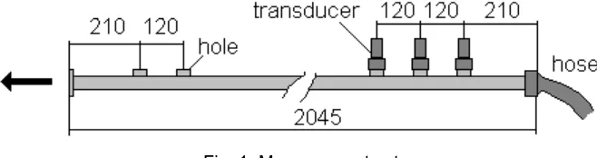
A few measurements were done on a φ27mm, 2mm thick steel pipe connected by a flexible

[image:3.595.125.454.308.395.2]

hose to a vibrator cooler fan (Goodmans V50). The free end of the pipe had 3 flute-like holes which could be individually opened or closed to control the flow of air through the pipe, Fig. 7. Three piezoelectric pressure transducers PCB 106B spaced by 120 mm were flush-mounted close to the pipe inlet. A 4-channel FFT card OROS 25 connected to a PC was used for spectrum analysis.

Fig. 1: Measurement set up

Measurements were done in five regimes resulting from different combinations of open holes:

regime end opening hole 1 hole 2

1 closed open closed

2 closed closed open

3 closed open open

4 open closed closed

5 closed closed closed

Table 1: Measurement regimes

Figure 2 show the RMS spectrum of pressure pulsations in regime 2, energy-averaged over 3 measurement positions. The tonal peak is at the blade passing frequency of the source.

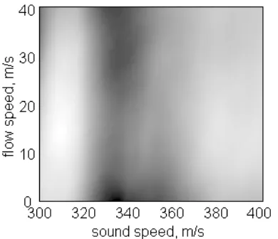
[image:3.595.166.430.568.743.2]

[image:4.595.107.485.112.308.2]

Fig. 3 shows the cost function C obtained from measurement data in regime 2, evaluated for the range of sound speed and flow velocity values. A distinct single peak is noticeable. The form of the function shows that clear identification of the sound speed and flow velocity is possible.

Fig. 3: Cost function C, regime 2

Fig. 4 shows the cost function for the first 4 regimes using the grey scale representation. The scale is normalized to 1, ranging from 1/25 to 1 on graphs 1-3 and from 1/18 to 1 on 4. The maximum, indicated by the crossing of the two dotted lines, shows the best fit value.

[image:4.595.89.507.386.725.2]

In parallel with acoustic measurements, the flow velocity was estimated using a hand-held anemometer, Testoterm 4400, complemented by an adapter to fit the holes and end opening. The temperature of the air inside the pipe was monitored by a small thermo probe. This enabled an estimation of sound speed in the pipe.

Table 2 gives the comparison of two groups of measurements. The discrepancy in flow velocity measurement could be attributed to some extent to errors induced by the anemometric technique used. The overall matching achieved between the acoustical and traditional measurements is seen to be very good, indicating the robustness of the developed method.

re g im e te m p e ra tu re ° C s p e e d o f s o u n d v ia t e m p e ra tu re r e a d in g s , m /s s p e e d o f s o u n d v ia a c o u s ti c m e a s u re m e n t, m /s fl o w v e lo c it y v ia a n e m o m e te r re a d in g s , m /s fl o w v e lo c it y v ia a c o u s ti c m e a s u re m e n t, m /s

1 25 347 346 18 17

2 25 347 348 18 17.5

3 27 348 349 26 26

[image:5.595.97.493.186.391.2]

4 27 348 348 36 34.5

Table 2: Comparison of measurement results on air-filled pipe.

By looking at Eq. (3), one can see that the function Θ becomes more and more error sensitive

the smaller the difference of the amplitudes of oppositely propagating waves. Thus conditions close to total acoustic reflection in the pipe will unfavourably affect results. This can be seen on

Fig. 4 which shows the C function plot for regime 5 where the pipe was fully closed. No distinct

[image:5.595.202.397.511.679.2]

maximum can be seen, the C function pattern being unevenly spread all over the parameter range. In fact, the difference between maximum and minimum values of the cost function is in this case a trivial 3,6% which is quite an unusable value.

Fig. 4: cost function for regime 5 (fully closed pipe)

While the first three regimes, i.e. the ones with closed end opening, produced sharp maxima, regime 4 produced instead a fairly smeared arc which peaked nevertheless at correct values of

c and v. The reason for this peculiarity can be seen on Fig. 5 showing the amplitude spectra of

Unlike in regimes 1-3, in regime 4 the difference of the amplitudes of oppositely propagating waves, obtained by a method described in [9], is small, thus ill conditioning the processing.

It should be pointed out that the use of a transducer array, as done in present measurements, generates undesirable coincidence effects at frequencies where the transducer spacing matches half the wavelength. Pressure spectra at frequencies at and close to the coincidence

frequencies, which at the transducer spacing of 0.12m were at ≈1450 Hz and ≈2900 Hz, were

[image:6.595.164.429.174.349.2]

consequently deleted from the processing.

Fig. 5: RMS spectra of positive (thick) and negative (thin line) propagating waves, regime 4.

CONCLUSIONS

A signal processing procedure is developed using the notion of a moving cross spectrum and a specific cost function. Experiments have demonstrated that this procedure is suitable for the identification of sound speed and flow velocity in fluid filled pipes.

REFERENCES

1. J.W. Verheij 1982, Multipath sound transfer from resiliently mounted shipboard machinery. Doctoral Thesis - Technische Physische Dienst TNO-TH, Delft.

2. J.W. Verheij 1990, Noise Control Engineering Journal 35, 69-76. Measurement of

structure-borne wave intensity on lightly damped pipes.

3. G. Pavic 1992, Journal of Sound and Vibration 154, 411-429. Vibroacoustical energy flow

through straight pipes.

4. C.A.F. de Jong and J.W. Verheij, 1993 Proceedings of the 4th International Congress on

Intensity Techniques, Senlis (France), 111-117. Measurement of vibrational energy flow in

straight fluid-filled pipes: a study of the effect of fluid-structure interaction.

5. C.A.F. de Jong 1994, Analysis of pulsations and vibrations of fluid-filled pipe systems. Doctoral Thesis - Technische Physische Dienst TNO-TH, Delft.

6. K. Trdak 1995, Vibration and acoustic intensity in pipes. Doctoral Thesis - Université de Technologie de Compiègne (in French).

7. L. Feng 1994, Journal of Sound and Vibration 176, 399-413. Acoustic properties of

fluid-filled elastic pipes.

8. L. Feng 1996, Journal of Sound and Vibration 189, 511-524. Experimental study of the

acoustic properties of a finite elastic pipe filled with water/air.

9.

G. Pavic 1997, Proceedings of Inter-Noise 97, Budapest, 2, 1513-1518. Analysis of