Probabilistic Graphical Models applied to Road Segmentation

Texto completo

(1)UAH. Probabilistic Graphical Models applied to Road Segmentation. Master Degree in Advanced Electronic Systems. Intelligent Systems Departament of Electronics Presented by: Mario Passani Montero. Advisor: Luis Miguel Bergasa Pascual. Alcalá de Henares, September 23th, 2015.

(2)

(3) A la memoria de María José Montero. “Hoy es siempre todavia.” Antonio Machado.

(4)

(5) ACKNOWLEDGEMENTS. En este punto, me gustaría dar las gracias a todas las personas que de una forma u otra han estado a mi lado, ayudándome a cumplir mis metas. Como soy un poco desastre y vosotros sois muchos, seguramente me olvide de alguien, confió en que no me lo tengáis en cuenta. A las primeras personas a las que debo mostrar mi más profundo agradecimiento son mi familia, especialmente a mi madre. Aunque me pesé bastante tu ausencia, pensar que estarías orgullosa de mi fue el importante aliento para trabajar, ir de un sitio para otro todo el día y estudiar una carrera (aunque me tiré algún que otro año de más y procastiné bastante, siendo sinceros). Muchas gracias a Luis Miguel Bergasa por lograr que entregue este trabajo y por contar conmigo para formar parte de un grupo de investigación puntero a nivel mundial, permitiéndome publicar en los principales congresos internacionales en el campo de los sistemas de transporte inteligente. Espero que no tengas en cuenta algún que otro deadline que me salté... Este agradecimiento se extiende a mis compañeros del grupo Robesafe: Roberto, Sergio, Edu y Javi. Vaya lata os he dado durante el año, seguro que ahora mejora la productividad a la par que disminuye el consumo de palmeras. Especial agradecimiento se merece Javi por las recomendaciones que me realizó para el paper del IV 2015, que fueron clave para que ganáramos el Best student paper award. Muchas gracias al resto de profesores del Departamento, especialmente a Felipe Espinosa por ser un crack como profesor, y a Rafa Barea por amenizarnos las mañanas con sus instructivas charlas futboleras. Este año he tenido varios trabajos, así que también tengo mucha gente a la que mostrar mi agradecimiento. Gracias a mis compañeros de la OTEC por el buen trato que siempre nos han dado, espero tener más desayunos y cañas con vosotros; a mis compañeros de CYTSA por darme la oportunidad de colaborar en un proyectos de ámbito internacional, por las catas de tartas y por el buen ambiente pese a la de horas y horas que echábamos; gracias a la gente de Telefónica por proponerme un trabajo tan interesante y por su buen ojo escogiendo a mis compañeros. Me queda mucha gente a la que mostrar mi agradecimiento: V.

(6) Acknowledgements. VI. A Andreas Geiger, Justin Domke, Jannik Fristch y Vladimir Haltakov por el intercambio de correos, que me ha permitido realizar un trabajo de mucha más calidad. A la gente de IEEE-ITSS por su reconocimiento a mi trabajo en el IV 2015. Muchas gracias también a José Alvarez por proponerme dar una minitalk y por su carta de apoyo. A Llorch, Mila, Maroto y demás universitarios con los que no coincide en ninguna clase. A David, Emilio, Miguel y demás universitarios con los que compartí demasiadas clases. A Blanca, por hacerme fan de Gran Hermano y a Roberto, por la compañía en las largas noches realizando trabajos (con la de tintos que tomábamos al final no han salido muy mal...). A Jacqueline, por seguir acordándose de mi pese estar en la otra punta del globo. A Esther, por sacar siempre un rato para quedar conmigo. A César por aguantar mis cosas de ni-ni. A Paco por preocuparte continuamente por mi pese a la distancia. A Luis por tus consejos de escalada y por el cariño que me ha mostrado siempre tu familia. ... Gracias a todos..

(7) RESUMEN. El futuro de los vehículos autónomos y de los sistemas avanzados de asistencia al conductor se sustenta en el desarrollo de sistemas de percepción capaces de proporcionar una detección rápida y precisa del entorno que rodea al vehículo. A pesar del largo trecho recorrido en el campo de detección de carretera, existe todavía un trecho importante en investigación para lograr incorporar capacidades de entendimiento de escena a los vehículos inteligentes. Este trabajo de fin de máster presenta un sistema de segmentación de carreteras a nivel de bit a partir de imágenes monoculares. La propuesta se basa en un modelo gráfico probabilístico y una serie de algoritmos y configuraciones seleccionadas oportunamente para acelerar el proceso de inferencia. En breve, el método propuesto emplea Conditional Random Fields y Uniformly Reweighted Belief Propagation. Por otro lado, el algortimo se valida en el dataset KITTI ROAD, alcanzando resultados en la línea del estado del arte pero con el tiempo de cómputo por imagen más bajo usando un PC estándar. Palabras clave: Probabilistic Graphical Models, Computer Vision, Conditional Random Fields, Machine Learning, Pater Recognition..

(8)

(9) ABSTRACT. The future of autonomous vehicles and driver assistance systems is underpinned by the need of fast and efficient approaches for road scene understanding. Despite the large explored paths for road detection, there is still a research gap for incorporating image understanding capabilities in intelligent vehicles. This Master thesis presents a pixelwise segmentation of roads from monocular images. The proposal is based on a probabilistic graphical model and a set of algorithms and configurations chosen to speed up the inference of the road pixels. In brief, the proposed method employs Conditional Random Fields and Uniformly Reweighted Belief Propagation. Besides, the approach is ranked on the KITTI ROAD dataset yielding stateof-the-art results with the lowest runtime per image using a standard PC Keywords: Probabilistic Graphical Models, Computer Vision, Conditional Random Fields, Machine Learning, Pattern Recognition..

(10)

(11) CONTENTS. Resumen. VII. Abstract. IX. Contents. XI. List of Figures. XV. List of Tables. XIX. List of Acronyms. XXII. List of Symbols. XXIV. 1. Introduction. 1. 1.1. Motivation . . . . . . . . . . . . . . . . . . . . . . . . . . . . . . . . . . . . . . . . .. 1. 1.2. Problems Associated . . . . . . . . . . . . . . . . . . . . . . . . . . . . . . . . . . .. 4. 1.3. Proposed Objectives . . . . . . . . . . . . . . . . . . . . . . . . . . . . . . . . . . .. 5. 1.4. Organization . . . . . . . . . . . . . . . . . . . . . . . . . . . . . . . . . . . . . . . .. 6. 2. State of Art. 7. 2.1. Marked Road Segmentation . . . . . . . . . . . . . . . . . . . . . . . . . . . . . . .. 9. 2.2. Unmarked Road Segmentation . . . . . . . . . . . . . . . . . . . . . . . . . . . . .. 14. 3. Graphical Models. 21. 3.1. Directed Models . . . . . . . . . . . . . . . . . . . . . . . . . . . . . . . . . . . . . .. 22. 3.2. Markov Random Fields. 24. . . . . . . . . . . . . . . . . . . . . . . . . . . . . . . . . ..

(12) CONTENTS. XII. 3.2.1. Conditional Random Fields . . . . . . . . . . . . . . . . . . . . . . . . . . .. 27. 3.2.1.1.. Parameterization . . . . . . . . . . . . . . . . . . . . . . . . . . . .. 28. 3.2.1.2.. The Three Basic Problems for Conditional Random Fields . . . .. 28. 3.3. Factor Graphs . . . . . . . . . . . . . . . . . . . . . . . . . . . . . . . . . . . . . . .. 29. 3.3.1. Inference in Factor Graphs . . . . . . . . . . . . . . . . . . . . . . . . . . . .. 31. 4. Preprocessing. 35. 4.1. Vanishing Point on the Horizon Detection . . . . . . . . . . . . . . . . . . . . . . .. 36. 4.1.1. Confidence-Weighted Texture Orientation Estimation . . . . . . . . . . . .. 36. 4.1.2. Locally Adaptive Soft-Voting . . . . . . . . . . . . . . . . . . . . . . . . . .. 39. 4.2. Determination of the ROI . . . . . . . . . . . . . . . . . . . . . . . . . . . . . . . .. 41. 5. CRF Model. 43. 5.1. Model Description . . . . . . . . . . . . . . . . . . . . . . . . . . . . . . . . . . . .. 44. 5.2. Software Structures Associated with the CRF Model . . . . . . . . . . . . . . . . .. 45. 6. Inference. 49. 6.1. Maximum Posterior Marginal Inference . . . . . . . . . . . . . . . . . . . . . . . .. 49. 6.2. Exponential Family . . . . . . . . . . . . . . . . . . . . . . . . . . . . . . . . . . . .. 51. 6.3. Variational Inference . . . . . . . . . . . . . . . . . . . . . . . . . . . . . . . . . . .. 52. 6.4. Tree-Reweighted Belief Propagation . . . . . . . . . . . . . . . . . . . . . . . . . .. 54. 6.4.1. Theoretical Basis . . . . . . . . . . . . . . . . . . . . . . . . . . . . . . . . .. 54. 6.4.2. Computation of Approximate Marginals . . . . . . . . . . . . . . . . . . .. 56. 7. Learning. 61. 7.1. Learning as Minimization of Empirical Risk . . . . . . . . . . . . . . . . . . . . . .. 62. 7.1.1. Loss functions . . . . . . . . . . . . . . . . . . . . . . . . . . . . . . . . . . .. 62. 7.1.1.1.. Univariate Logistic Loss . . . . . . . . . . . . . . . . . . . . . . .. 63. 7.1.1.2.. Univariate Conditional Quadratic Loss . . . . . . . . . . . . . . .. 63. 7.1.1.3.. Clique Logistic Loss . . . . . . . . . . . . . . . . . . . . . . . . . .. 64. 7.2. Back Tree-Reweighted Belief Propagation . . . . . . . . . . . . . . . . . . . . . . .. 64.

(13) CONTENTS 8. CRF Potentials. XIII. 67. 8.1. Introducing Features in the Model . . . . . . . . . . . . . . . . . . . . . . . . . . .. 67. 8.2. Node Features . . . . . . . . . . . . . . . . . . . . . . . . . . . . . . . . . . . . . . .. 70. 8.2.1. Color Patches . . . . . . . . . . . . . . . . . . . . . . . . . . . . . . . . . . .. 70. 8.2.2. Position . . . . . . . . . . . . . . . . . . . . . . . . . . . . . . . . . . . . . .. 72. 8.2.3. Histogram of Oriented Gradients . . . . . . . . . . . . . . . . . . . . . . . .. 72. 8.2.4. Local Binary Patterns . . . . . . . . . . . . . . . . . . . . . . . . . . . . . . .. 76. 8.2.5. Summary . . . . . . . . . . . . . . . . . . . . . . . . . . . . . . . . . . . . .. 77. 8.3. Edge Features . . . . . . . . . . . . . . . . . . . . . . . . . . . . . . . . . . . . . . .. 78. 8.3.1. Bias Feature . . . . . . . . . . . . . . . . . . . . . . . . . . . . . . . . . . . .. 79. 8.3.2. Difference Intensities Discretized . . . . . . . . . . . . . . . . . . . . . . . .. 79. 8.3.3. Different Parametrization of Vertical and Horizontal Links . . . . . . . . .. 79. 8.3.4. Summary . . . . . . . . . . . . . . . . . . . . . . . . . . . . . . . . . . . . .. 80. 9. Post-processing. 81. 9.1. Elimination of small specks misclassified as “road” . . . . . . . . . . . . . . . . .. 82. 9.2. Elimination of small specks misclassified as “off-road” . . . . . . . . . . . . . . .. 85. 10. Experimental Results. 87. 10.1. KITTI Road Dataset . . . . . . . . . . . . . . . . . . . . . . . . . . . . . . . . . . . .. 87. 10.2. Set Up the Classification Model . . . . . . . . . . . . . . . . . . . . . . . . . . . . .. 89. 10.2.1. Semantic Labeling in Miniaturized Scenes . . . . . . . . . . . . . . . . . .. 91. 10.2.2. Selection of Optimal Edge Appearance Probability Parameter . . . . . . .. 92. 10.2.3. Influence of Loss Functions . . . . . . . . . . . . . . . . . . . . . . . . . . .. 93. 10.2.4. Influence of Pre- and Post-processing stages . . . . . . . . . . . . . . . . .. 94. 10.3. Comparative with State of Art . . . . . . . . . . . . . . . . . . . . . . . . . . . . . .. 94. 10.3.1. Urban Marked Lanes . . . . . . . . . . . . . . . . . . . . . . . . . . . . . . .. 95. 10.3.2. Urban Unmarked Lanes . . . . . . . . . . . . . . . . . . . . . . . . . . . . .. 95. 10.3.3. Urban Multiple Marked Lanes . . . . . . . . . . . . . . . . . . . . . . . . .. 95. 11. Conclusions and Future Works. 101. 11.1. Conclusions . . . . . . . . . . . . . . . . . . . . . . . . . . . . . . . . . . . . . . . . 101 11.2. Future works . . . . . . . . . . . . . . . . . . . . . . . . . . . . . . . . . . . . . . . . 102 Bibliography. 105.

(14)

(15) LIST OF FIGURES. 1.1. Annual number of fatalities, injury accidents and injured people in EU-27, 20012010. . . . . . . . . . . . . . . . . . . . . . . . . . . . . . . . . . . . . . . . . . . . .. 2. 1.2. Share of fatalities by area type in EU-21, 2010. . . . . . . . . . . . . . . . . . . . . .. 2. 1.3. Car equipped with various ADAS. . . . . . . . . . . . . . . . . . . . . . . . . . . .. 4. 1.4. System block diagram showing the main steps in our road extractor. Down and up arrows correspond with the downsample and upsample performing with superpixels . . . . . . . . . . . . . . . . . . . . . . . . . . . . . . . . . . . . . . . . .. 5. 2.1. Example of a urban marked road with its associated ground truth . . . . . . . . .. 8. 2.2. Example of a “harder” urban marked road with its associated ground truth . . .. 8. 2.3. Example of a urban unmarked road with its associated ground truth . . . . . . .. 8. 2.4. Marked road vs. unmarked road. . . . . . . . . . . . . . . . . . . . . . . . . . . . .. 9. 2.5. Images illustrating an example of the difference between lane and road detection. 10 2.6. Example of lane-marking detection using HSV color model. . . . . . . . . . . . .. 10. 2.7. Example of lane-marking algorithm output using a camera mounted on top of a truck cabin. . . . . . . . . . . . . . . . . . . . . . . . . . . . . . . . . . . . . . . . . .. 11. 2.8. Result of road detection in a curved roads in color-based road segmentation. . .. 11. 2.9. The camera, road and image co-ordinate systems. . . . . . . . . . . . . . . . . . .. 12. 2.10. Results of lane segmentation based on steerable filters. . . . . . . . . . . . . . . .. 13. 2.11. Image with bad contrast but well marked lane boundaries using splines. . . . . .. 13. 2.12. B-Snake based lane model. . . . . . . . . . . . . . . . . . . . . . . . . . . . . . . . .. 13. 2.13. Example of lane detection process at night with DriveSafe . . . . . . . . . . . . . .. 14. 2.14. Nonhomogenous and complex road shape example. . . . . . . . . . . . . . . . . .. 15. 2.15. Road detection examples. . . . . . . . . . . . . . . . . . . . . . . . . . . . . . . . .. 16.

(16) XVI. LIST OF FIGURES. 2.16. Several examples of vanishing point estimation and road model extraction. . . .. 16. 2.17. Road segmentation using the vanishing point. . . . . . . . . . . . . . . . . . . . .. 16. 2.18. Blocks generated of frame of road scene. . . . . . . . . . . . . . . . . . . . . . . . .. 17. 2.19. Segmentation unmarked road based on optical flow. . . . . . . . . . . . . . . . . .. 17. 2.20. System block diagram showing the main processing steps in the SPRAY ego-lane extractor. . . . . . . . . . . . . . . . . . . . . . . . . . . . . . . . . . . . . . . . . . .. 18. 2.21. Distribution of base points over the metric space (left) and the SPRAY feature generation procedure illustrated for one base point (right). . . . . . . . . . . . . .. 18. 2.22. Block diagram of a probabilistic distribution approach to road segmentation. . .. 19. 2.23. Stanley, the robot who won the DARPA challenge. . . . . . . . . . . . . . . . . . .. 20. 3.1. Examples of directed graphical model and undirected graphical model . . . . . .. 23. 3.2. Example of a direct graphical model. . . . . . . . . . . . . . . . . . . . . . . . . . .. 23. 3.3. Example of a undirect graphical model. . . . . . . . . . . . . . . . . . . . . . . . .. 25. 3.4. Example of conditional independence . . . . . . . . . . . . . . . . . . . . . . . . .. 26. 3.5. The concept of parameterization . . . . . . . . . . . . . . . . . . . . . . . . . . . .. 28. 3.6. Example of a factor graph. . . . . . . . . . . . . . . . . . . . . . . . . . . . . . . . .. 30. 3.7. Factor graph associated to a undirected graphical model . . . . . . . . . . . . . .. 30. 3.8. A factor graph specifying a conditional distribution . . . . . . . . . . . . . . . . .. 30. 3.9. Examples of message flows associated with the inference process . . . . . . . . .. 32. 3.10. One possible leaf to root message schedule in the sum-product algorithm. . . . .. 33. 3.11. One possible root to leaf message schedule in the sum-product algorithm. . . . .. 33. 4.1. Rectangular mask filters out non-road expected pixels and the ROI contains the road. The horizon line is estimated from a set of training images. . . . . . . . . .. 35. 4.2. Gabor wavelets with 5 scales and 36 orientations. . . . . . . . . . . . . . . . . . .. 37. 4.3. Response of a Gabor filter for an input gray image. . . . . . . . . . . . . . . . . . .. 37. 4.4. Illustration of the problem in vanishing point estimation by conventional voting strategy . . . . . . . . . . . . . . . . . . . . . . . . . . . . . . . . . . . . . . . . . . .. 40. 5.1. Portion of the a pairwise grid-like Conditional Random Field in a 4 neighbor system. . . . . . . . . . . . . . . . . . . . . . . . . . . . . . . . . . . . . . . . . . . .. 44. 5.2. Graph of the CRF model aligned with the ROI. . . . . . . . . . . . . . . . . . . . .. 44. 5.3. Simplified structure of the random field to implement message passing algorithms. 45 5.4. Absorption of observed random variables . . . . . . . . . . . . . . . . . . . . . . .. 45. 6.1. Pipelines corresponding to training and inference. . . . . . . . . . . . . . . . . . .. 50.

(17) LIST OF FIGURES. XVII. 6.2. Differences between graph, tree and spanning tree. . . . . . . . . . . . . . . . . .. 55. 6.3. Illustration of the spanning tree polytope . . . . . . . . . . . . . . . . . . . . . . .. 56. 6.4. Pairwise grid like CRF and one example of spanning tree associated with it. . . .. 56. 6.5. Flow of messages between variable nodes to factor nodes and vice versa. . . . . .. 57. 8.1. Portion of the proposed graphical model. The node and edge features are overlaid in blue and red, respectively. . . . . . . . . . . . . . . . . . . . . . . . . . . . .. 68. 8.2. Example of a pairwise CRF aligned with the ROI of a road scene. . . . . . . . . .. 68. 8.3. Concatenation of node feature functions to obtain the matrix F . . . . . . . . . . .. 69. 8.4. The node features in each node are calculated on the observation in the same node. 70 8.5. Examples of an scene splitting in their RGB channels . . . . . . . . . . . . . . . .. 71. 8.6. Cone model of HSV space. . . . . . . . . . . . . . . . . . . . . . . . . . . . . . . . .. 72. 8.7. Examples of an scene splitting in their HSV channels . . . . . . . . . . . . . . . .. 73. 8.8. Normalized position feature . . . . . . . . . . . . . . . . . . . . . . . . . . . . . . .. 73. 8.9. An overview of the HOG features extraction chain. . . . . . . . . . . . . . . . . .. 74. 8.10. Calculation of the gradients in the HOG algorithm. . . . . . . . . . . . . . . . . .. 75. 8.11. Orientation binning in HOG . . . . . . . . . . . . . . . . . . . . . . . . . . . . . . .. 75. 8.12. Blocks and cells in HOG . . . . . . . . . . . . . . . . . . . . . . . . . . . . . . . . .. 75. 8.13. The result of applying the HOG algorithm to a road scene . . . . . . . . . . . . .. 76. 8.14. An example of local binary pattern computation. . . . . . . . . . . . . . . . . . . .. 76. 8.15. Examples of different combinations of P and R in LBP. . . . . . . . . . . . . . . .. 77. 8.16. The result of applying the LBP algorithm to a road scene . . . . . . . . . . . . . .. 77. 8.17. The edge features are calculated between nodes associated with the latent variables. . . . . . . . . . . . . . . . . . . . . . . . . . . . . . . . . . . . . . . . . . . . .. 78. 8.18. Bias and variance contributing to total error. As the model complexity is increased, the variance tends to increase and the squared bias tends to decrease in a bias-variance tradeoff . . . . . . . . . . . . . . . . . . . . . . . . . . . . . . . . . .. 79. 9.1. Labeling of a road scene with some pixel misclassified . . . . . . . . . . . . . . . .. 81. 9.2. Use of morphological erosion for removing salt noise. . . . . . . . . . . . . . . . .. 84. 9.3. Example of morphological dilation. . . . . . . . . . . . . . . . . . . . . . . . . . . .. 84. 9.4. Removal of false positives using a morphological opening. . . . . . . . . . . . . .. 85. 9.5. Use of morphological dilation for eliminating holes. . . . . . . . . . . . . . . . . .. 86. 9.6. Removal of false negatives using a morphological closing . . . . . . . . . . . . . .. 86. 10.1. KITTI Vision Benchmark Suite submission process . . . . . . . . . . . . . . . . . .. 88.

(18) XVIII. LIST OF FIGURES. 10.2. Visualization of state-of-the-art evaluation metrics. . . . . . . . . . . . . . . . . . .. 88. 10.3. Randomization of the location of the samples in k-fold cross validation. . . . . .. 90. 10.4. 5-fold cross validation . . . . . . . . . . . . . . . . . . . . . . . . . . . . . . . . . .. 90. 10.5. Example of road detection in the same road scene by using different loss functions. 93 10.6. Examples of images illustrating the performance of the method in the category UM Road. . . . . . . . . . . . . . . . . . . . . . . . . . . . . . . . . . . . . . . . . .. 96. 10.7. Example of images in BEV illustrating the performance of the method in the category UM Road. . . . . . . . . . . . . . . . . . . . . . . . . . . . . . . . . . . . .. 96. 10.8. Example of images in perspective view illustrating the performance of the method in the category UU Road. . . . . . . . . . . . . . . . . . . . . . . . . . . . .. 97. 10.9. Example of images in BEV illustrating the performance of the method in the category UU Road. . . . . . . . . . . . . . . . . . . . . . . . . . . . . . . . . . . . .. 97. 10.10.Example of images in perspective view illustrating the performance of the method in the category UMM Road. . . . . . . . . . . . . . . . . . . . . . . . . . .. 98. 10.11.Example of images in BEV illustrating the performance of the method in the category UMM Road . . . . . . . . . . . . . . . . . . . . . . . . . . . . . . . . . . .. 99.

(19) LIST OF TABLES. 10.1. Road estimation results obtained for different sizes of the validation images. All results are in %. . . . . . . . . . . . . . . . . . . . . . . . . . . . . . . . . . . . . . .. 91. 10.2. Sweep of values for the ρ parameter in the TRW inference. KITTI ROAD images at 20% resolution. . . . . . . . . . . . . . . . . . . . . . . . . . . . . . . . . . . . . .. 92. 10.3. Comparison of loss functions on KITTI ROAD. . . . . . . . . . . . . . . . . . . . .. 93. 10.4. Influence of pre- and post-processing stages. . . . . . . . . . . . . . . . . . . . . .. 94. 10.5. Road estimation results on the test set images . . . . . . . . . . . . . . . . . . . . .. 95. 10.6. Comparison of KITTI URBAN-ROAD state-of-the-art . . . . . . . . . . . . . . . .. 95.

(20)

(21) LIST OF ACRONYMS. ADAS. Advanced Driver Assistance Systems.. ANN. Artificial Neural Network.. Back TRW. Back Tree-Reweighted Belief Propagation.. BEV. Bird’s Eye View.. BFGS. Broyden Fletcher Goldfarb Shanno algorithm.. BN. Bayesian Network.. CRF. Conditional Random Field.. DGM. Directed Graphical Model.. FFT. Fast Fourier Transform.. FG. Factor Graph.. FN. False Negative.. FP. False Positive.. GPU. Graphical Processor Unit.. HOG. Histogram of Oriented Gradients.. IPM. Inverse Perspective Mapping.. ITS. Intelligent Transport Systems.. IU. Image Understanding.. LASER. Light Amplification by Stimulated Emission of Radiation.. LBP. Local Binary Pattern..

(22) List of Acronyms. XXII. LDWS. Lane Departure Warning System.. LIDAR. LIght Detection And Ranging.. LKAS. Lane Keeping Assist Systems.. LUT. Look Up Table.. MAP. Maximum A Posteriori.. MPM. Maximum Posterior Marginals.. MRF. Markov Random Field.. NP. Non-deterministic Polynomial-time.. PGM. Probabilistic Graphical Model.. RADAR. RAdio Detection And Ranging.. ROI. Region of Interest.. SIFT. Scale Invariant Feature Transform.. SPRAY. Spatial Ray.. SVM. Support Vector Machines.. TN. True Negative.. TP. True Positive.. TRW. Tree-Reweighted Belief Propagation.. UGM. Undirected Graphical Model.. UM. Urban Marked Two-way Road.. UMM. Urban Marked Multi-Lane Road.. UU. Urban Unmarked..

(23) LIST OF SYMBOLS. ψi. Unary potential.. ψij. Pairwise potential.. A. Log partition function.. ⊥⊥. Conditional independence.. D ∆. Dataset.. ∅. The empty set.. F. Matrix consist of all observation feature function for nodes.. fj. Factor j from a factor graph.. fk. Observation feature function k − th for nodes.. f k (yv , x). Node feature function k − th for node yv .. G. Matrix consist of all observation feature function for edges.. gk. Observation feature function k − th for edges.. gk ( y u , y v , x ). Edge feature function k − th for nodes yu and yv .. H. Entropy.. [[·]]. Function evaluating to 1 if its argument is true, to 0 otherwise.. J. Unit matrix or number or edges features (according to the context).. Loss functions..

(24) List of Symbols. XXIV. K. Number of observation feature function for nodes.. L. Local polytope.. M. Marginal polytope.. nC. Number of cliques in the graph.. Ni. The set of neighbors of Xi .. Ω. Null matrix.. P. Number of samples in a dataset.. πi. The parents index of node i in a directed graphical model.. ψc. Clique potential.. U (y, y0 ). Utility function measuring the satisfaction of a output predicted.. w. Parameters of the graphical model.. X Xi xi x. Input domain (a set of images). A random variable, or the node for Xi in a graph. A realization of random variable Xi . A realization of the random variable X = ( X1 , X2 , . . . , Xn ) (observed superpixels in an image).. Y y. Output domain (labels assign to the superpixels). A realization of the random variable Y = (Y1 , Y2 , . . . , Yn ) (classes asigned to the superpixels in an image).. Z. The partition function..

(25) CHAPTER. 1 INTRODUCTION. This work is framed with the research line of the Intelligent Transport Systems (ITS) developed by the Robesafe group at the University of Alcalá comprised of professors and researchers ascribed to the Department of Electronics. More specifically, the work is inscribed within the domain of real-time computer vision for Advanced Driver Assistance Systems (ADAS) and autonomous driving, being a contribution to initiatives trying to avoid that a vehicle get out of its ego-lane involuntary. In brief, this project presents an approach to semantic interpretation of scene, Image Understanding (IU), using a embedded system on-board vehicle to classify objects in real time. The core task of our proposal can be regarded as pixel labeling problem. Labeling, just as name implies, labels each pixel (or pixel block) in its category. In our case, the label set has two elements: road and off-road, so the systems performs real time road detection. Road detection is a key requirement for the successful development and use of intelligent vehicles due to its many potential practical applications, especially in ADAS (example of such ADAS are Lane Departure Warning System (LDWS), Lane Keeping Assist Systems (LKAS), automatic parking, etc.) and autonomous driving. In order to carry out the proposal, we apply an innovative technique of machine learning, namely Conditional Random Fields (CRFs) [1]. Recent advances in discrete optimization and probabilistic graphical models have become CRFs in a standard tool for segmenting and labeling task.. 1.1.. Motivation. Road transport plays a vital role in the modern society, allowing economic growth, social development and prosperity. According to official data by European Union [2] people travel mainly by road, with private cars accounting for 73% of passenger traffic and about 44% of goods transported in the EU go by road..

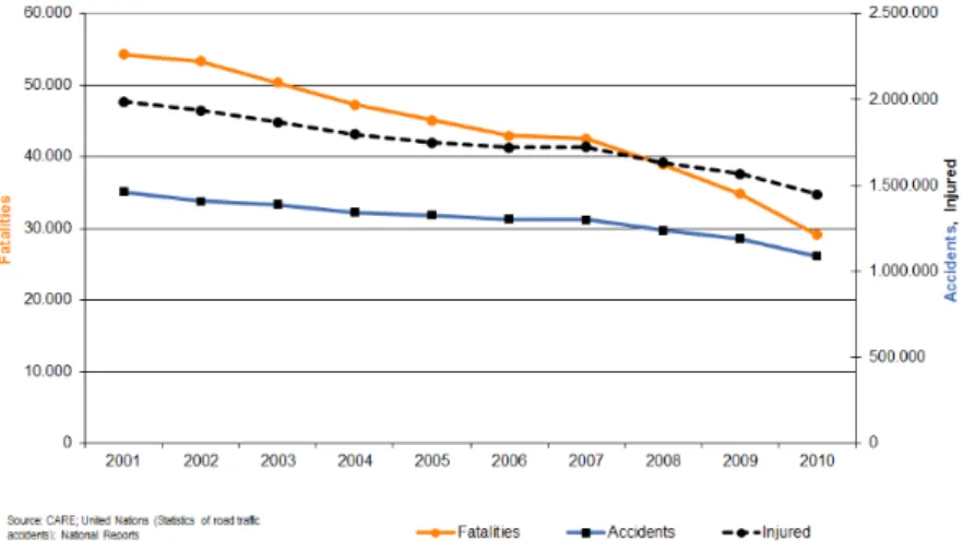
(26) 2. Chapter 1. Introduction However, the road transport is facing a number of challenges. Examples include but no are. limited to: traffic accidents, congested roads, the constant rise in the price of fuel, air pollution, etc. Even though there have been advances to address the above-mentioned challenges, the numbers are startling. Thus, there were still more than 31,000 deaths on European Roads in 2010 [3]. In the Figure 1.1 we show the annual number of fatalities, injury accidents and injured people in the European Union [4].. Figure 1.1: Annual number of fatalities, injury accidents and injured people in EU-27, 20012010. According to the Figure 1.2, most accidents do no occur in motorways, but they occur in urban area and rural roads. In both cases, drivers can benefit from a road detection system due to the worse signaling conditions of rural roads and the challenging urban traffic with continuous lane changes.. Figure 1.2: Share of fatalities by area type in EU-21, 2010. In the last years, due to these alarming facts, the automotive industry is introducing different systems, including systems for active and passive safety to improve the security conditions and achieve a more efficient driving. Perhaps one of the most representative examples are the ADAS [5] that provide real time help to the driver. According to several surveys [6], ADAS can prevent up to 40% of traffic accidents, depending on the type of ADAS and the type of accident scenario. The ADAS can cover a wide range of systems, from systems that provide information or warnings, to system involved in the vehicle control and manoeuvrings tasks. Examples of.

(27) 1.1 Motivation. 3. ADAS are: Adaptive cruise control. Adaptive light control. Automatic parking. Blind spot detection. Collision avoidance system, also knows as pre-cash system. Driver drowsiness detection. Electric vehicle warning sounds. Hill descent control. Intelligent speed adaptation. Lane change assistance. Lane departure warning system. Night vision. In the Figure 1.3 we show an example of a car equipped with some of the ADAS listed above. Nonetheless, the introduction of ADAS on the market is slow. In our opinion, the primary cause of low market penetration is the economic added cost together with the lack of information about these systems. If we look carefully the ADAS listed above, we note that the most of them use computer vision techniques to detect the presence of possible objects and classify them. Therefore, we can conclude that a way to enhance the use of ADAS can involves to develop cheaper systems capable to perform IU easily installed on different vehicles. In research and development these systems based on computer vision have grown significantly in importance, due to their advantages over other detection sensors or location technologies. The following are the main advantages identified by Guan [7]: They are relatively inexpensive and can be easily installed on a vehicle, and they can detect and identify objects without the need for complementary companion equipment. These systems can capture a tremendous wealth of visual information over wide areas, often beyond the longitudinal and peripheral range of other sensors such as RAdio Detection And Ranging (RADAR) or Light Amplification by Stimulated Emission of Radiation (LASER)..

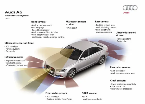
(28) 4. Chapter 1. Introduction. Figure 1.3: The Audi A6 is an example of premium car equipped with several moderns ADAS. The continuous innovations in computer vision processing algorithms allows to exploit the wealth of visual data captured by cameras, identifying more subtle changes and distinctions between objects, enabling a wide range of ever more driving safety systems. Besides, the use of a monocular system, despite the obvious limitations to geometric reconstruction, has significant advantages over stereoscopic systems due to lower cost, computational requirements and technical complexity.. 1.2.. Problems Associated. The general problem of detecting objects in images is very complex because it involves the development of a system capable of distinguishing a particular class of objects from the rest. Our system shall operate correctly over marked roads, like highways, and over unmarked road, that are common in rural areas and inner-city. Therefore, due to the great diversity of environments in which our system must work, we have to deal with a number of issues: Low visibility due to inclement weather, including overcast sky, heavy rain, etc. Presence of noise in the images. Occlusions produced by obstacles such other vehicles. Extensive shady zones..

(29) 1.3 Proposed Objectives. 5. Variations in the appearance of the material of the road (asphalt, gravel, etc.) and possible wear down. The mobile nature of the work platform adds complexity to the problem.. Furthermore, road detection must be not only as accurate as possible but also prompt. In order to have a practical system, classification in real time is mandatory.. 1.3.. Proposed Objectives. The objectives pursued that we wish to achieve in this work are the followings:. Development of an algorithm for road segmentation based on CRFs introduced by Lafferty et al. [1]. Selection of the most appropriate model for the CRF. Selection of the best visual descriptors for the segmentation road problem. Validation of the proposed using the KITTI Road dataset, the most known public dataset for evaluating road area and ego-lane detection approaches [8]. Documentation of the method developed. Report conclusions and propose future works.. A overall description of the system designed is depicted in the Figure 1.4. The remainder of the book explains in detail each one of the different stages.. Figure 1.4: System block diagram showing the main steps in our road extractor. Down and up arrows correspond with the downsample and upsample performing with superpixels.

(30) 6. Chapter 1. Introduction. 1.4.. Organization. This dissertation is structured as follow: Chapter 2 : Reviews related state of art on road segmentation. Chapter 3: This chapter presents a basic introduction to graphical models. Directed and undirected graphical models are described, giving particular emphasis to CRFs. It also described the tool factor graphs. Chapter 4: This chapter describes the preprocessing followed to obtain the Region of Interest (ROI) in where the CRF will be built. Chapter 5: We justify the choice of the implemented model and describe in detail the skeleton of our CRF, showing some of the required structures for its implementation. Chapter 6: This chapters concerns the necessary process to inference the road in a given image. In our case, the graph of the CRF is not tree-structured, which implies that probabilistic inference is NP-hard. However, we can effectively approximate by some message passing algorithm. Chapter 7: Here we detailed the learning task. That is, the process required to obtain the parameters of the model. In this work we use a recent approach presented by Justin Domke [9] to do parameter learning using approximate marginal inference instead the usual approach based in approximations of the likelihood. Chapter 8: Describes the feature functions used in our model distinguishing between node and edge features. This chapter is key due the choice of appropriate features that determine the success or failure of the classifier. Chapter 9: This chapter describes the post-processing based on morphological operations to slightly increase the overall accuracy. Chapter 10: We present and discuss the results of the segmentation on the KITTI Road datasets presented above, carrying out an comparative evaluation against the state of art. Chapter 11: Concludes the dissertation and discusses possible future directions that are not covered by this work..

(31) CHAPTER. 2 STATE OF ART. Road segmentation is a well-known problem in ITS that has been studied for decades [10]. However, the emergence of new systems such as ADAS (e.g., lane departure warning, adaptative cruise control, lane keeping, lane centering, turn assist), personal navigators, autonomous driving, etc. has caused a renewed interest in this issue because most of these systems need to detect the road surface ahead the ego-vehicle. The potential uses for road scene segmentation are very varied [11] such as discard large image areas, impose geometrical constraints on objects in the scene, etc. Thus, a variety of systems has been developed to detect the road in some kind of environment. They used different sensors to acquire the information of the environment, such as, monocular vision, stereo vision, laser range finders and fusion of some of them [12]. Although the road detection problem, does not look like a hard one, this impression is misleading. The significant gaps in research, high reliability demands and large diversity in case conditions make that the building a useful road segmentation system is a large scale research and development effort [10]. On well marked roads, especially highways, road detection can easily been done by detecting the lane marking. However, general road detection is much more challenging due to many reasons, some of which are: Arbitrary road shape. Absence of lane markings. Occlusions with other vehicles and objects. Variations in the type and shape of the road. Variations in lighting conditions with the daytime. It also can occur when the vehicle is passing through a tunnel..

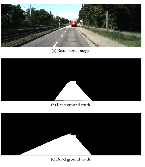
(32) 8. Chapter 2. State of Art Variations in the appearance of the material asphalt, gravel, etc.. Its includes phe-. nomenons like wear down and switch from one road to another. Variations depending on acquisition conditions. The clutter of background. In order to show the variability of some of the conditions mentioned above we show some road scenes in Figures 2.1, 2.2 and 2.3. The road segmentation, as we can see, is an easy task only in some specific cases.. (a) Road urban scene image. (b) Ground truth. Figure 2.1: Example of a urban marked road and its associated ground truth taken from [8]. In this case the road segmentation is relatively straightforward.. (a) Road urban scene image. (b) Ground truth. Figure 2.2: Example of a “harder” urban marked road and its associated ground truth taken from [8]. In this case the road segmentation is further complicate.. (a) Road urban scene image. (b) Ground truth. Figure 2.3: Example of a urban unmarked road and its associated ground truth taken from [8]. The case is more complex due to the absence of lane marks and the presence of shadows. For these reason, when addressing the study of state of art in road segmentation is appropriate to distinguish two types of roads because there are different approaches most appropriated for each case, namely: 1. Marked, like highways and highway-like roads (Figure 2.4a). 2. Unmarked, that are common in rural areas and inner-city (Figure 2.4b). A particular case of road segmentation is the ego-lane segmentation that involves detect and extract the lane in which the vehicle is currently driving on. This is an important question in.

(33) 2.1 Marked Road Segmentation. 9. (a) Marked road. (b) Unmarked road. Figure 2.4: Marked road vs. unmarked road. the design of ADAS because these systems should avoid to invade the opposite lane. In the Figure 2.5 we show the difference between lane and road detection for the same road scene.. 2.1.. Marked Road Segmentation. In order to segment the marked road scenes there are highly diverse techniques. However, the localization of road markings is the most used approach [13–16]. Methods based upon segmenting the road using the color cue have also been proposed but they do not work well for general road image, specially when the roads have little difference in colors between their surface and the environment. In addition, laser, radar and stereovision have also been used for structured-road detection. For example, [14] Sun et al. propose a method for lane-marking detection which is carried out by color analysis of road scene images using hue-saturation-intensity [17] color model achieving better results that using RGB color model. A example is depicted in Figure 2.6. The approach of Felisa and Zani [13] produces reliable results exploiting a robust polyline matching technique capable of running at soft real-time rates. They employs an Inverse Perspective Mapping (IPM) transformation [18]. The Figure 2.7 shows a example of lane-marking using this approach. Kuo-Yu and Sheng-Fuu Lin [19] use similar ideas. Firstly, they choose a ROI to find out a threshold using statistical method in a color image. Then, this threshold will be used to distinguish possible lane boundaries from the road. They use a color-based segmentation to find out the lane boundary. Since in the real world, lane marking is extensional vertically, they propose use a quadratic function to approach the lane marking because it may be interpreted as a kind of parabolic. This algorithm can deal with solid or broken line, straight or curved line, obstacle on lane marking, other traffic signs drawn on the road, road pavement, shadow,.

(34) 10. Chapter 2. State of Art. (a) Road scene image.. (b) Lane ground truth.. (c) Road ground truth.. Figure 2.5: Images illustrating an example of the difference between lane and road detection.. (a) Example of input image.. (b) Final result.. Figure 2.6: Example of lane-marking detection using HSV color model taken from [14]..

(35) 2.1 Marked Road Segmentation. 11. Figure 2.7: Example of lane-marking algorithm output using a camera mounted on top of a truck cabin taken from [13]. and sun light reflection. The system proposed demands low computational cost and memory requirements and is robust in the presence of noise, shadows, pavement and obstacles like cars, motorcycles and pedestrians. Yingua He et al. [20] present a road-area detection algorithm based on color images. Their algorithm is composed of two modules: In the first module, an edge image of the road scene is analyzed to obtain the candidates for road borders and to delimit the area that will subsequently be used to compute the mean and variance of the Gaussian distribution, assumed to be obeyed by the color components of road surfaces. The second module effectively extracts the road area and reinforces boundaries that most appropriately fit the road-extraction result. The combination of these modules can overcome basic problems due to inaccuracies in edge detection based on the intensity image alone and due to the computational complexity of segmentation algorithms based on color images. Figure 2.8 depicts an example of road detection.. Figure 2.8: Result of road detection in a curved roads in color-based road segmentation [20]. Southall and Taylor [21] present a method for estimating road shape using a single on board color camera, together with inertial and velocity information. They use a six-dimensional state vector s[k] to describe both the position of the vehicle and the geometry of the road:.

(36) 12. Chapter 2. State of Art. s(t) = [y0 (t), tan e(t), C0 (t), C1 (t), W (t), θ (t)] T. (2.1). where y0 denotes the lateral offset and e the bearing of the vehicle with respect to the centreline of the lane, C0 and C1 the curvature and rate of change of curvature of the lane ahead of the vehicle, W the width of the lane, and θ the pitch of the camera to the road surface, which is assumed to be locally flat. Then, given a state s(t) Equation (2.2) describes the shape of the road ahead of the vehicle: y( x ) = y0 + tan (e) x +. C0 2 C1 3 x + x 2 6. (2.2). where y is the lateral position of the road centre with respect to the vehicle, and x the distance ahead, as illustrated in Figure 2.9.. Figure 2.9: The camera, road and image co-ordinate systems in [21]. To extract the lane marks they run a Hough transform [22] algorithm whereas the road shape is estimated using a particle filter [23]. Bin and Jain[24] also use a Hough transform to extract the lane-markings. Another quite different approach is presented by McCall and Trivedi [16], they propose to use steerable filters [25] for robust and accurate lane-marking detection. According to the experiments carried out by the authors, steerable filters provide an efficient method for detecting a wide variety of lane markings under varying lighting and road conditions. In this way, steerable filters help in providing robustness to complex shadowing, lighting changes from overpasses and tunnels, and road-surface variations. Moreover, steerable filters are computational simples, allowing a a fast implementation. Figure 2.10 depicts some examples of lane segmentations. An alternative approach is based on the use of splines [26] to fit the limits of the roads. For example, Kaske et al [27] propose using Chi-Square fitting combined with random search to obtain the best set of parameters of a deformable template corresponding with the lane boundaries; an example of lane segmentation can be found in Figure 2.11. A similar approach is presented by Jung and Kelber [28] but using linear-parabolic splines. Finally, Wang et al. [15] proposed a lane detection and tracking algorithm able to describe a wide range of lane structures using B-snakes, an economical realization of snakes (also knows as active contours) by using far fewer state variables by cubic B-Splines as is depicted in Figure 2.12. Although the cost of vehicle safety technology is dropping, most safety technologies are not available in economy vehicles and it will be a decade before the vast majority of cars on the.

(37) 2.1 Marked Road Segmentation. 13. Figure 2.10: Results of lane segmentation based on steerable filters. Scenes from dawn (row 1), daytime (row 2), dusk (row 3), and nighttime (row 4). These scenes show the environmental variability caused by road markings and surfaces, weather, and lighting.. Figure 2.11: Image with bad contrast but well marked lane boundaries using splines. Figure 2.12: The model of left image uses 3 control points and the model of the right uses 4 control points..

(38) 14. Chapter 2. State of Art. road today have these safety features built-in. contrast, smartphone solutions can be used in all vehicles (new or old) and represent a cheap and disruptive technology. This is the reason why in the last years there has been an active work on using smartphones to assist drivers. One clear example that can be cited is DriveSafe, an safety app presented by Bergasa et al. [29] that detects inattentive driving behaviors and gives corresponding feedback to drivers, scoring their driving and alerting them in case their behaviors are unsafe. This works employs a modification of the Dickmans clothoidal road model-based method [30] to evaluate drowsiness. In brief, the app detects the lane following this steps: 1. Transformation of the image to gray scale. 2. Creation of two ROIs, one for the left markings and another for the right one 3. Detection of edges in the ROIs using an adaptive Canny algorithm which maximizes the edges in each ROI. 4. Elicitation of candidate lines for each of the two ROIs using the Hough transform together with some geometrical constraints. 5. Election of a representative line per ROI maximizing the length of the line, minimizing the angle difference between the candidate and the road model and the difference between the model vanishing point and the vanishing point obtained among the candidates for the left and the right side. Figure 2.13 shows an example of these steps for a lane detection process at night.. Figure 2.13: Example of lane detection process at night with DriveSafe a) ROIs in the gray scale image, b) Canny edges, c) Segmented and winner lines, d) Marker measures and lane model.. 2.2.. Unmarked Road Segmentation. For unstructured roads and structured roads without remarkable boundaries, road segmentation must be addressed from an alternative perspective to detection based on lane-markings..

(39) 2.2 Unmarked Road Segmentation. 15. Methods based upon segmenting the road using color cue have also proposed but they do not work well when the roads have little difference in colors between their surface and the environment, may failing with strong shadows and highlights. Sotelo et al. [31] propose to use the color features of the HSI color space as the basis for performing the segmentation of nonstructured road. The HSI color space segments the image by using the cylindrical distribution of its color feature. The approach presented by Tan et al. [32] uses color classification and learning to construct and use multiple road and background models. These color models are used to segment each color image into road and background by estimating the probability that a pixel belongs to a particular model. Since the color models are constructed on a frame by frame basis. The color model proposed by the authors uses normalized R and G because they are fairly robust to changes in illumination, while at the same time being fast to calculate. An example of detection is depicted in Figure 2.14.. Figure 2.14: Nonhomogenous and complex road shape example. Upper-left shows the raw image of an intersection; bottom-left is the current road probability, bottom-right is the temporal fusion, and upper-right is the segmented road. Álvarez and López [33] propose an approach to vision-based road detection robust to shadows. Their approach relies on using a shadow-invariant feature space combined with a modelbased classifier. The model, a simple likelihood-based classifier, is built online to improve the adaptability of the algorithm to the current lighting and the presence of other vehicles in the scene. The Figure 2.15 depicts some road detection examples using this approach. When there are little difference in color between the road and offroad areas, it is hard to find a intensity change to delimit state. The most plausible solution is using the texture. For example Nieto and Salgado [34] use a steerable filter bank to extract different edge images, then an enhanced edge image is composed with these images resulting in a clear identification of the lane markings. Finally, a fast Hough transform and minimum squares fitting find the best vanishing point of the image and the lane markings that delimit the road. The approaches of Rasmussen [35] and Kong et al. [36] (see 2.17) are pretty similar to this strategy but using Gabor filters to estimate the vanishing point. In all of these cases, the road segmentation is robust to variations in the illumination and the type of road. However, may fail with curved road, heavy traffic and strong shadow edges..

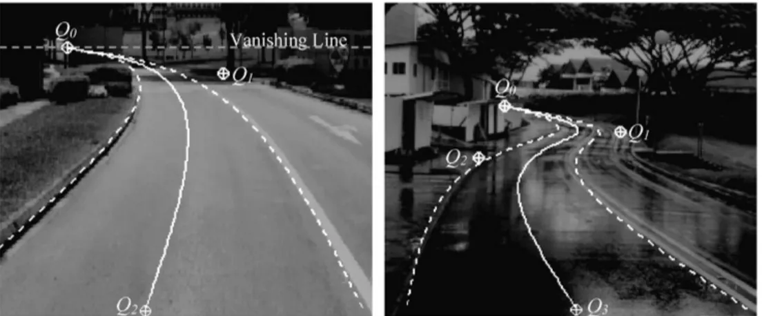
(40) 16. Chapter 2. State of Art. Figure 2.15: Road-detection examples. (Top row) Original image. (Second row) Illuminantinvariant image. (Third row) Detected road. (Bottom row) Comparison against handsegmented result. (Yellow) Correctly classified pixels. (Green) Falsely detected road pixels. (Red) False background pixels.. Figure 2.16: Several examples of vanishing point estimation and road model extraction. Example (a) shows the most simple case where the road is almost empty, while cases (b) and (c) are quite more difficult as there are overtaking traffic and road traffic signals that difficult the correct detection. Case (d) shows a particular situation where the illumination conditions have abruptly changed due to the shadow casted by a bridge on the road.. Figure 2.17: Road segmentation using the vanishing point..

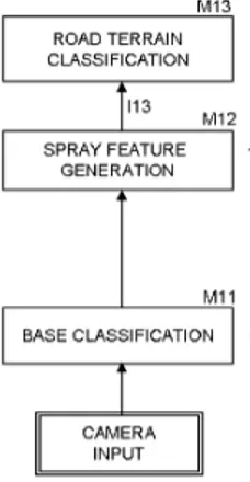
(41) 2.2 Unmarked Road Segmentation. 17. The color and texture is used in [37] employing Artificial Neural Networks (ANNs). This work employs a block-based classification method consists on dividing the image in blocks of pixels and evaluate them as a single unit. A value is generated to represent this group, this value can be the average of the RGB, entropy and others features from collection of pixels represented (see Figure 2.18. The main disadvantage of this system is that the roads can present aperiodic texture, which is hard to characterize.. Figure 2.18: Blocks generated of frame of road scene. For each block, a feature value is calculated depending on the feature chosen. This strategy has been used to reduce the amount of image elements, allowing faster processing. Lookingbill et al. [38] propose using reverse optical flow to provide an adaptive segmentation of the road scene finding examples of a ROI at previous time in the past. However, the method does not work well when the camera is unstable and the estimation of the optical flow is not robust enough. Some scene frames are depicted in Figure 2.19.. Figure 2.19: Segmentation unmarked road based on optical flow. For unstructured roads and structure road without remarkable boundaries and markings, Alon et al. [39] propose a realtime system combining Adaboost [40] classification to form an initial segmentation with the texture boundaries constrained by geometric projection to find the road area for each frame. The work of Kühnl et al. [41] is one of the approaches that achieves better results in the KITTI online evaluation website [8] (see 10) working in real time at the expense of use a powerful Graphical Processor Unit (GPU).Their proposed system aims at detecting ego-lanes in cases of both explicit (lane-markings or curbstones) and implicit (unmarked road) delimiters. For that, the system represents visual properties of both, the road surface and delimiting elements in confidence maps based on analyzing local visual features. On such confidence maps, Spatial Ray (SPRAY) that incorporate properties of the global environment are calculated. The system, depicted in the workflow of Figure 2.20, consists of three parts:.

(42) 18. Chapter 2. State of Art. Figure 2.20: System block diagram showing the main processing steps in the SPRAY ego-lane extractor. 1. Base classification. A set of three base classifiers (boundary, road and marking), which work on preprocessed camera images create three confidence maps in a metric representation (using IPM). Different training strategies are used to specialize each classifier on its specif task. 2. SPRAY feature generation. Takes a confidence map from a base classifier and extracts a spatial feature vector for a defined number of points. Using radial vectors called rays the spatial layout with respect to the confidence map is captured at each individual point. A ray vector Rα includes all confidence values along a line with a certain angular orientation α. The SPRAY features corresponds with the locations where the ray value reaches a certain threshold. All the individual features computed from the different base classifiers are merged to obtain a spatial feature vector for each base point. The Figure 2.21 shows a confidence map of one base classifier in the metric space and the SPRAY feature generation process.. Figure 2.21: Distribution of base points over the metric space (left) and the SPRAY feature generation procedure illustrated for one base point (right). 3. Road terrain classification once the classifier is trained using GentleBoost [42], the system can process input images with the learned parameters. All works that we have been mentioned rely on monocular vision. The stereo vision based approaches use disparity map acquired through stereo matching. Then the disparity map can.

(43) 2.2 Unmarked Road Segmentation. 19. be analyzed to get the free space and the road. Labayrade et al. [43] present an approach based on the construction and investigation of the “v-disparity” image which provides a good representation of the geometric content of the road scene. Vitor et al. [44] create a set of probabilistic models using an adapted version of the Joint Boosting algorithm [45] with Texton (color and 2D texture) and Diston (3D information based on disparity map) feature maps. Essentially, the method consists on a set of weak classifiers analyzing the information according to Figure 2.22. Although this work achieves state-of-the-art results for the road segmentation, the classifier requires 2.5 minutes for each frame. In general, these methods need dense stereo matching which is time consuming and the error increases with the distance.. Figure 2.22: Block diagram of a probabilistic distribution approach to road segmentation. Recently, several LIght Detection And Ranging (LIDAR) based road detection algorithms have been developed. This kind of methods use the accurate 3D location of the LIDAR points to analyze the scene and take the flat area as the road. For example, Thrun et al. incorporate LIDAR in the Stanley robot to detect nondrivable terrain a sufficient range to stop or take the appropriate evasive action [46]. Stanley is equipped with five single-scan laser range finders mounted on the roof, tilted downward to scan the road ahead. Figure 2.23a illustrates the scanning process. Each laser scan generates a vector of 181 range measurements spaced 0.5 ◦ apart. Projecting these scans into the global coordinate frame according, to the estimated pose of the vehicle, results in a 3D point cloud for each laser. Figure 2.23b shows an example of the point clouds acquired by the different sensors. Moosmann et al. [47] present a graph-based approach to segment ground and objects from 3D LIDAR scans using a ngeneric criterion based on local convexity measures. Experiments show good results in urban environments including smoothly bended road surfaces. Chen et al. presents a algorithm for real-time segmenting three-dimensional scans of various terrains. An individual terrain scan is represented as a circular polar grid map that is divided into a number of segments. A one-dimensional Gaussian Process regression with a non-stationary covariance function is used to distinguish the ground points or obstacles in each segment. Thus, the proposed approach splits a large-scale ground segmentation problem into many simple Gaussian.

(44) 20. Chapter 2. State of Art. (a) Illustration of a laser sensor: The sensor is angled downward to scan the terrain in front of the vehicle as it moves. Stanley possesses five such sensors, mounted at five different angles.. (b) Each laser acquires a threedimensional 3D point cloud over time. The point cloud is analyzed for drivable terrain and potential obstacles.. Figure 2.23: Stanley, the robot who won the DARPA challenge. Process regression problems with lower complexity, and can then get a real-time performance while yielding acceptable ground segmentation results. Moreover, a recent work by R. Mohan [48] combines Deep Deconvolutional and Convolutional Neural Networks for the general task of scene parsing. Compared to different engineered features election methods, this is an alternative technique to automatically learn features directly from the images. This method is currently ranking first on KITTI ROAD benchmark. However, this approach is computationally intensive and it requires a GPU cluster to process the data..

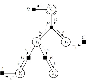
(45) CHAPTER. 3 GRAPHICAL MODELS. The theory behind this work is essentially framed in the context of IU. The purpose of IU is, as its name suggests, to enable the machine to understand the world through performing complex reasoning on useful information extracted from processing of digital signals. Mathematically, let x denote the observed data, typically the pixels or superpixels of an image, belonging to an input domain X and let y denote a vector of interest from an output domain Y that corresponds to a mathematical answer to the IU problem. Thus, IU can be formulated as finding a mapping from y to x [49]. For example, given an image, we would like to classify all objects in their class, which is essentially an inverse problem [50]. To this end, we often need to build a model of the real world that relates observed measurements to quantities of interest [51]. Unfortunately, several difficulties emerged in the modeling due to the fact that most of the vision problems are inverse, ill-posed and require a large number of latent and/or observed variables to express the expected variations of the answer [52]. Furthermore, the observed signals are usually noisy, incomplete and often only provide a partial view of the desired space in most cases. Probabilistic Graphical Models (PGMs), usually referred to simply as graphical models, can help us to facing these situations. They combine harmoniously probability theory and graph theory towards a natural and powerful formalism for modeling and solving inference and estimation problems in various engineering fields [53]. A graphical model consists of a graph where each node (also called vertices) is associated with a random variable (or group of random variables) and an edge (also known as link or arcs) between a pair of nodes encodes probabilistic interaction between the corresponding variables. The absence of an edge between two variables represents conditional independence between those variables [52]. Conditional independence [54] means that two random variables a and b are independent given a third random variable c if and only if the conditional joint can be written as a product of conditional marginals, that is: a, b ⊥⊥ c ⇔ p( a, b|c) = p( a|c) p(b|c). (3.1).

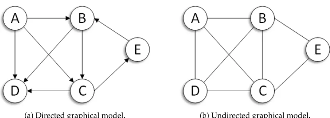
(46) 22. Chapter 3. Graphical Models. where we are using the notation a, b ⊥⊥ c to indicate that a and b are conditionally independent given c. It is noteworthy that in contrast two random variables a and b are statistically independent if and only if p( a, b) = p( a) p(b). Conditional independence is an important concept because it makes densities modular reducing the space required to represent densities, allowing us to to decompose complex probability distributions into a product of factors, each consisting of the subset of corresponding random variables. Thus, the complex computations required for inference can be carried out much more efficiently by using message-passing algorithms [51]. PGMs are powerful tools for visualizing the independence properties of complex probability models. They offers several useful properties, we can look at some of the more important ones identified by Bishop [53]: They provide a simple way to visualize the structure of a probabilistic model and can be used to design and motivate new models. Insights into the properties of the model, including conditional independence properties, can be obtained by inspection of the graph. Complex computations, required to perform inference and learning in sophisticated models, can be expressed in terms of graphical manipulations, in which underlying mathematical expressions are carried along implicitly. Two types of graphical models are popular: 1. Directed Graphical Models (DGMs), also known as Bayesian Networks (BNs), in which the edges of the graphs have a source and a target provided by the particular directionality indicated by arrows. An example is depicted in Figure 3.1a. 2. Undirected Graphical Models (UGMs), also known as Markov Random Fields (MRFs), in which the links do not carry arrows and have no directional significance. Figure 3.1b shows an example. In practice, directed graphs are better at expressing causal generative models whereas undirected graphs are better at representing soft constraints between variables. Sections 3.1 and 3.2 will provide a brief overview of both models. For the purposes of solving inference problems, it is often convenient to convert both directed and undirected graphs into a different representation called factor graph [51]. Section 3.3 introduces this kind of representation.. 3.1.. Directed Models. Directed Graphical Models (DGMs) [55] can be described using a directed graph G = (V , E ) which consists of a set V = { X1 , X2 , . . . , X N } of nodes and a set E = { Xi , X j } of edges [53]..

(47) 3.1 Directed Models. 23. (a) Directed graphical model.. (b) Undirected graphical model.. Figure 3.1: Examples of directed graphical model, also knows as Bayesian network, and undirected graphical model, also knows as Markov random field.. Each node represents a random variable Xi (for simplicity, we refer to a variable and its node interchangeably as Xi ) whose realization we denote as xi whereas edges indicate possible dependencies between these random variables. A DGM describe a family of probability distributions according to the Equation (3.2): N. p(x) =. ∏ p ( xi | x π ) i. (3.2). i =1. where πi indexes the parent nodes of Xi , that is to say, the sources of incoming edges to Xi (sometimes πi may be the empty set). This key equation expresses the factorization properties of the joint distribution for a directed graphical model.. Figure 3.2: Example of a direct graphical model. An example of directed model describing a set of five random variables is shown in Figure 3.2. This graphical structure implies the following parent relationships: π1 = ∅, π2 = {1}, π3 = π4 = {2} and π5 = {3, 4}. Using Equation (3.2) this yields the following factorization:. p ( x1 , x2 , x3 , x4 , x5 ) = p ( x1 ) p ( x2 | x1 ) p ( x3 | x2 ) p ( x4 | x2 ) p ( x5 | x3 , x4 ). (3.3). To interpret the meaning of (3.3), our starting point is the factorization produced using the standard chain rule of probabilities. The chain rule allows us to factories a joint distribution into a product of distributions. One possible factorization according to chain rule of probabilities is:.

(48) 24. Chapter 3. Graphical Models. p ( x1 , x2 , x3 , x4 , x5 ) = p ( x1 ) p ( x2 | x1 ) p ( x3 | x1 , x2 ) p ( x4 | x1 , x2 , x3 ) p ( x5 | x1 , x2 , x3 , x4 ). (3.4). This represents the joint distribution over X as the product of five distributions. When we compare (3.4) with (3.3), we notice that a number of conditioning variables are omitted in Equation (3.3). For example, the third term p( x3 | x2 ) has missed x1 from its conditioning context. This omission represents a conditional independence relation, encoding our knowledge about the lack of inter-relatedness between the variables, and thus simplifies the joint probability distribution. We can determine if a conditional independence X ⊥⊥ Y |{ Z1 , . . . , Zk } holds by appealing to a graph separation criterion called d-separation, which stands for direction-dependent separation [56]. X and Y are d-separated if there is no active path between them. Although the formal definition of active paths is somewhat involved, the set of active paths independence relations can be found using the Bayes’ Ball algorithm [57], which analyzes paths connecting these sets of variables for possible sources of dependence. Directed models are usually used to model causal relationships between random variables and have been applied in many fields such as computer vision, artificial intelligence, automatic control, etc. In computer vision, Hidden Markov Models [58] and Kalman Filters [59], two subsets of directed models, are popular in different tasks such as object tracking [60], denoising [61], motion analysis [62], sign language recognition [63], etc. due to its ability to model causal relationships. Neural networks [64] are other type of directed models that provide an important machine learning method to deal with vision problems [65].. 3.2.. Markov Random Fields. MRFs models [55,66] are useful in modeling a variety of phenomena where one cannot naturally to ascribe a directionality to the interaction between variables. For example modeling an image, it is plausible to suppose that the intensity values of neighboring pixels are correlated; however, being forced to choose a direction for the edges, as required by a DGM, is rather awkward. Furthermore, the undirected models also offer a different and often simpler perspective on directed models, in terms of both independence and structure and the inference task. Undirected models represent a different factorization of the joint distribution to that of directed models, and with different conditional independence semantics. They are described by an undirected graph G = (V , E ), where V = { X1 , X2 , . . . , X N } are the nodes and E = { Xi , X j } are the undirected edges. This graphical structure describe a family of probability distributions according to Hammersley-Clifford [67] theorem, which states that: p(x) =. 1 Z. ∏ ψc (xc ). such that ψc ( xc ) > 0 ∀c ∈ C. (3.5). c∈C. where Z is the normalizing partition function; ψc ( xc ) denotes the potential function of a clique c,.

(49) 3.2 Markov Random Fields. 25. which is a positive real-valued function on the possible configuration xc of the clique c, and C denotes a set of cliques contained in the graph G. The kind of probability distribution specified in Equation 3.5 is usually called a Gibbs (or Boltzmann) distribution [52].. Figure 3.3: Example of a undirect graphical model. The term clique describes a subset of nodes of an undirected graph such that its induced subgraph is complete; that is, every two distinct nodes in the clique are adjacent (i.e., connected by an edge). A maximal-clique is a clique that cannot be enlarged with additional nodes while still remaining fully connected. For example, the graph in Figure 3.3 contains the following cliques:. { X1 } , { X2 } , { X3 } , { X4 } { X5 } , { X1 , X2 } , { X2 , X3 } , { X2 , X4 } , { X3 , X4 } , { X3 , X5 } , { X4 , X5 } , { X2 , X3 , X4 } and { X3 , X4 X5 }. Out of these, only are maximal cliques: { X1 , X2 },{ X2 , X3 , X4 } and { X3 , X4 X5 }, in these three cliques we can subsume all the remaining cliques in the graph. If the potential functions, ψc , for each non-maximal clique is incorporated into the potential function of exactly one of its subsuming maximal cliques, the product of 3.5 can be limited to only maximal cliques without any loss of generality [68]. The partition function Z in (3.5) ensures that p(x) is correctly normalized, i.e. ∑ x p(x) = 1, being a valid probability distribution. This is achieved by summing out the numerator in (3.5) for every possible realization: Z , ∑ ∑ . . . ∑ ∏ ψc ( xc ) x1 x2. (3.6). x N c∈C. where each clique c indexes a subset of the variables in x, as defined by its edges in the graph. This large summation arises as a direct consequence of the mostly unconstrained potential functions, ψ, in (3.5). Directed graphical models use conditional probability distributions as their potential functions and thus they need no normalization (i.e., Z = 1). However, this constant is not necessarily one for undirected models, and often proves intractable to calculate. This is because it requires summing over a number of realizations which is exponential in the number of random variables (if we have n discrete nodes in our graph having k possible states, then the evaluation of the normalization term involves summing over k M states). For sparsely connected graphs, this summation can be made more efficient by dynamic programming [69]. The Hammersley-Clifford theorem applied to the graph G = (V , E ) factored in accordance to the Equation (3.5) gives two further outcomes of interest: 1. Local Markov property: If Ni is the set of neighbors of Xi (i.e., those nodes which are connected to Xi by an edge) in G, then p( xi |x\ xi ) = p( xi |N ( Xi )). Thus, we can easily see that.

(50) 26. Chapter 3. Graphical Models two nodes are conditionally independent given the rest if there is no direct edge between them. 2. Global Markov property: If we have three disjoints subsets of nodes, denoted A, B and. C , we state that A ⊥⊥ B|C when the set C separates A and B in the graphical model. In others words, all paths connecting A to B must pass through the node C . This is considerably simpler than the semantics for directed graphs, described in Section 3.1. Figure 3.4 illustrates an example of this property.. Figure 3.4: An example of an undirected graph in which every edge from any node in set A to any node in set B passes through at least one node in set C . Consequently the conditional independence property A ⊥⊥ B|C holds for any probability distribution described by this graph. An alternative representation avoids the positivity constraints in the potentials in Equation (3.5) by using the model known as the Gibbs distribution [70]. Thus, we can define an energy function expressing each potential function in Equation (3.5) as follows:. ψc ( xc ) = exp (− E( xc )). (3.7). We can now rewrite Equation (3.5): 1 p(x) = Z. 1 ∏ exp (−E(xc )) = Z exp − ∑ E(xc ) c∈C c∈C. ! (3.8). In this way, finding the state x with the highest probability can now be seen as an energy minimization problem, with the benefit that the exponential can be moved outside the product. The most used approach is to define the log-potentials as a linear function of the parameters of the model: log ψc ( xc ) , φc ( xc )T wc. (3.9). where φc ( xc ) is a feature vector derived from the values of the variables xc and wc is a vector of model parameters. It is important to note that the potentials are not probabilities. Rather, they represent the relative “compatibility” between the different assignments to the potential. This allows (3.5) to be re-parametrized over only thelog-potentials:.

(51) 3.2 Markov Random Fields. 27. p(x) =. 1 exp ∑ φc ( xc )T wc Z c∈C. (3.10). The importance of Equation (3.10) is that allows characterize the global probability by the log-potential functions defined over maximal cliques, being completely unconstrained.. 3.2.1.. Conditional Random Fields. We often have access to measurements that correspond to variables that are part of the model. In that case we can directly model the conditional distribution [51] p(y|x) where x denote the observations that are always available and y is a tuple of latent variables (usually corresponds with the labels). This can be expressed compactly using CRFs [1]. A CRF is simply a conditional distribution p(y|x) with an associated Undirected Graphical Model (UGM); it can be viewed as an MRF which is globally conditioned on the observed data x. Accordingly, CRFs inherit global and local Markov properties. The major difference between these two is that MRFs are generative, i.e. model p(y, x), while CRFs are discriminative, i.e. model p(y|x). Because the model is conditional, the dependencies among the input variables x do not need to be explicitly represented, affording the use of rich, global features of the input graphical structure [71]. In this way, we can draw our attention on modeling what we are really concern to us, namely the distribution of labels given the observations. Generally, CRFs can be written as: p(y|x) =. 1 ψc (yc , x) such that ψc (yc , x) > 0 ∀c ∈ C Z (x) c∏ ∈C. (3.11). We emphasize that the realization of random variables yi are conditioned on the input x and that the potential function depends on the entire input and not only subsets of the input. CRFs have been applied to various works in computer vision. For example, CRFs are used to model spatial dependencies in the image [72], to solve object class image segmentation [73, 74] and to jointly estimate the class category, location, and segmentation of objects/regions from 2D images [75]. Because in many computer vision problem the most common and fundamental type of interaction between pairs of variables is pairwise , the most used type of CRFs is the pairwise CRFs. In a pairwise CRF the Equation (3.11) is factorized into a sum of potential functions defined on cliques of order strictly less than three. In this way, we explicitly differentiate between types of potentials (unary and pairwise). The conditionally probability is then defined as follows: p(y|x) =. 1 ψi (yi , x) ∏ ψij (yi , y j , x) Z (x) i∏ ∈V (i,j)∈E. where ψi refers to the unary potentials whereas ψij refers to the pairwise potentials.. (3.12).