Published online: February 19, 2016
GEOMETRIC PROPERTIES OF NEUTRAL SIGNATURE METRICS ON 4-DIMENSIONAL NILPOTENT LIE GROUPS
TIJANA ˇSUKILOVI ´C
Abstract. The classification of left invariant metrics of neutral signature on the 4-dimensional nilpotent Lie groups is presented. Their geometry is ex-tensively studied with special emphasis on the holonomy groups and projec-tive equivalence. Additionally, we focus our attention on the Walker metrics. They appear as the underlying structure of metrics on the nilpotent Lie groups with degenerate center. Finally, we give complete description of the isometry groups.
Introduction
The geometry of 4-dimensional Lie groups with a left invariant metric has been studied extensively through the years. For a comprehensive treatment and for references to the extensive literature on the subject of left invariant metrics on Lie groups in small dimensions one may refer to the book [2]. Initially motivated by works of Lauret, Cordero, and Parker, we became interested in the case of the nilpotent Lie groups. The first classification type results for small dimensions in the positive definite setting are due to Milnor [31] who classified 3-dimensional Lie groups with a left invariant positive definite metric. Riemannian nilmanifolds of dimension three and four were extensively studied by Lauret [26], while for dimension five we refer to [22]. The distinction between Riemannian and pseudo-Riemannian settings is obvious from the results of Rahmani [34]. It is shown there that on the 3-dimensional Heisenberg group H3 there are three classes of
non-equivalent Lorentz left invariant metrics, one of which is flat. In the positive definite case there is only one class and it is not flat. The classification of the Lorentz 3-dimensional nilpotent Lie groups was done by Cordero and Parker [10], while the classification in the 4-dimensional case can be found in [7].
A metric g of split (2,2) signature is said to be a Walker metric if there exists a 2-dimensional null distribution which is parallel with respect to the Levi-Civita connection ofg. This type of metrics has been introduced by Walker [36], who has
2010Mathematics Subject Classification. 53B10, 53B30, 53C22, 22E25.
Key words and phrases. nilpotent Lie group, holonomy group, Walker metrics, geodesically equivalent metrics, isometry groups.
shown that they have a (local) canonical form depending on three smooth func-tions. Walker metrics appear in a natural way being associated with tangent and cotangent bundles in various constructions (for more details on geometric proper-ties of Walker metrics we refer to [8], [9] and references therein). Here they arose as the underlying structure of the metrics on the nilpotent Lie groups with degenerate center.
The other question of interest is a projective equivalence of left invariant metrics. The first examples of geodesically equivalent metrics are due to Lagrange [25]. Later, Beltrami [4] generalized this example to the metrics of constant negative curvature, and to the case of pseudo-Riemannian metrics of constant curvature. Though the examples of Lagrange and Beltrami are 2-dimensional, one can easily generalize them to every dimension and to every signature.
Intuitively, one might expect a link between projective relatedness and a holo-nomy type, since if∇= ¯∇, then (M, g) and (M,g) have the same holonomy type.¯ Indeed, holonomy theory can, to some extent, describe projective equivalence (see the work of Hall [19, 20, 37]).
Matveev gave an algorithm for obtaining a list of possible geodesically equivalent metrics to a given metric. It is interesting that the proposed algorithm does not depend on the signature of the metric. Manifolds of constant curvature allow geodesically equivalent metrics (see [25], [4], etc.). Sinjukov [35] showed that all geodesically equivalent metrics given on a symmetric space are affinely equivalent. For more comprehensive results in this area we refer to [24], [29], [30] and references therein.
Another striking difference between the Riemannian and pseudo-Riemannian set-up is apparent from the isometry group information. In particular, it can be significantly larger than in the Riemannian or pseudo-Riemannian case with non-degenerate center. It was shown that in the Riemannian case the group of isometric automorphisms coincides with the group of isometries of the 2-step nilpotent Lie groupN fixing its identity element and the distribution
T N =υN⊕ξN. (1)
These subbundles are obtained by the left translation of the splitting at the Lie algebra leveln=υ⊕ξ, wheren is the Lie algebra ofN,ξ denotes its center and υthe orthogonal complementary subspace ofξ. Further information regarding the positive definite case can be found in [14] and [23].
Lie groups acting by isometries on a fixed pseudo-Riemannian 2-step nilpotent Lie group endowed with a left invariant metric —the group of isometric automor-phisms, the group of isometries preserving the splitting (1), and the full isometry group— were investigated by Cordero and Parker in [11] and later by del Barco and Ovando in [12]. In the same paper, del Barco and Ovando also considered bi-invariant metrics on the 2-step nilpotent Lie groups, showing that there are isometric automorphisms not preserving any kind of splitting.
G4 is presented. This completes the full classification of metrics on the nilpotent
Lie groups in dimensions three and four.
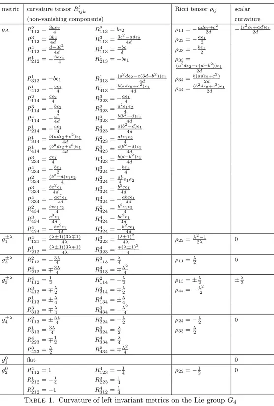
In Section 2 the geometry of the metrics is explored. The curvature tensor (Tables 1 and 2) and the holonomy groups (Table 3) were calculated. Also, we study a connection between holonomy groups and projective equivalence of metrics. It is interesting that if the center of the group is degenerate, the corresponding metric is of Walker type. We focus our attention on these metrics.
In Section 3 we find projective classes of the metrics (Theorems 3.1 and 3.2). Furthermore, we solve the problem of the projectively equivalent metrics on the 4-dimensional nilpotent Lie groups by showing that a left invariant metricgis ei-ther geometrically rigid or has projectively equivalent metrics that are also affinely equivalent (Theorem 3.3). Moreover, all affinely equivalent metrics are left invari-ant, while their signature may change.
Finally, Section 4 provides complete description of the isometry groups for both H3×RandG4.
1. Classification of non-equivalent inner products of neutral signature
Let (N, g) be a nilpotent Lie group with a left invariant metricg. If not stated otherwise, we assume thatN is 4-dimensional and that the metric g is of neutral signature (+,+,−,−).
Magnin [27] proved that, up to isomorphism, there are only two non-abelian nilpotent Lie algebras of dimension four: h3⊕Randg4, with corresponding simply
connected Lie groupsH3×RandG4.
With respect to the basis{x1, x2, x3, x4}, the Lie algebrah3⊕Ris defined by a non-zero commutator
[x1, x2] =x3.
The Lie algebrah3⊕Ris 2-step nilpotent with a 2-dimensional centerZ(h3⊕R) =
L(x4, x3) and a 1-dimensional commutator subalgebra spanned byx3.
The Lie algebrag4, with respect to the basis{x1, x2, x3, x4}, is given by non-zero
commutators
[x1, x2] =x3, [x1, x3] =x4.
The Lie algebrag4is 3-step nilpotent with a 1-dimensional centerZ(g4) =L(x4)
and a 2-dimensional commutator subalgebra
g04:= [g4,g4] =L(x3, x4).
Denote byAut(n) the group of automorphisms of the Lie algebranthat is defined by
Aut(n) :={F :n→n|F linear, bijective, [F x, F y] =F[x, y], x, y∈n}.
Denote byS(n) the set of non-equivalent neutral inner products (i.e. of signature (+,+,−,−)) of the Lie algebra n. Having a basis of the Lie algebra n fixed, the set S(n) is identified with symmetric matrices S of signature (2,2) modulo the following action of the automorphism group:
S7→FTSF, F∈Aut(n). (2)
Automorphisms of these Lie groups are described in the following two lemmas.
Lemma 1.1. [26]The groupAut(g4)of automorphisms of the Lie algebrag4, with respect to the basis{x1, x2, x3, x4}, consists of real matrices of the form
Aut(g4) =
a1 0 0 0
a2 b2 0 0
a3 b3 a1b2 0
a4 b4 a1b3 a21b2
ai ∈R, i= 1, . . . ,4, bj∈R, j= 2, . . . ,4, a1, b26= 0
.
Lemma 1.2. [26] The group Aut(h3⊕R) of automorphisms of the Lie algebra
h3⊕R, with respect to the basis {x1, x2, x3, x4}, consists of real matrices of the form
Aut(h3⊕R) =
A 0 0
b1 detA µ
b2 0 λ
A∈GL(2,R), b1, b2∈R2, λ, µ∈R, λ6= 0
.
It is interesting to notice that in the Riemannian case, up to equivalence (2), there is just one inner product for each Lie algebra (see [26]). Note that the situation in the Lorentz case is quite different — there are seven families of inner products in the case of the Lie algebra g4 and six families in the case of h3⊕R (see [7]).
Theorem 1.1. The setS(g4)of non-equivalent inner products of neutral signature on the Lie algebrag4, with respect to the basis{x1, x2, x3, x4}, is represented by the following matrices:
SA=
1 0 0 0
0 2 0 0
0 0 a b
0 0 b c
, 1, 2∈ {−1,1},
S1±λ=
∓1 0 0 0
0 0 0 1
0 0 ±λ 0
0 1 0 0
, S2±λ=
0 0 0 1
0 ∓1 0 0
0 0 ±λ 0
1 0 0 0
S3±λ=
0 0 1 0
0 ∓1 0 0
1 0 0 0
0 0 0 ±λ
, S4±λ=
∓1 0 0 0
0 0 1 0
0 1 0 0
0 0 0 ±λ
,
S10=
0 0 0 1
0 0 1 0
0 1 0 0
1 0 0 0
, S20=
0 0 1 0
0 0 0 ±1
1 0 0 0
0 ±1 0 0
,
withλ >0. MatrixA=
a b
b c
has split(+,−)signature if16=2, and(+,+) (respectively(−,−)) signature if 1=2=∓1.
Proof. The proof is entirely analogous to the case of Lorentz signature (see [7]). Denote the center ofg4 byZ =L(x4) and the commutator subalgebra byg04= L(x3, x4). Let us consider a signature ofg04.
For the signatures (+,+), (−,−) and (+,−), we get the inner productsSA (for
an appropriate choice of1, 2).
If g04 is partially degenerate, we distinguish two cases: when the center is null
(inner productsS1±λ andS2±λ) and when it is not (inner productsS±λ3 andS4±λ). Let us examine more thoroughly the case wheng0
4 is totally null. The matrixS
representing the inner product reduces to
S=
p r e f
r q g h
e g 0 0
f h 0 0
.
Since the action ofF ∈Aut(g4) cannot change the signature of the elementh, after some calculation one can show that forh= 0 one gets the inner productS10 and forh6= 0 there exist two non-equivalent inner products represented byS20.
Theorem 1.2. The set S(h3 ⊕R) of non-equivalent inner products of neutral
signature on the Lie algebra h3⊕R, with respect to the basis {x1, x2, x3, x4}, is represented by the following matrices:
Sµ± =
∓1 0 0 0
0 ∓1 0 0
0 0 ±µ 0
0 0 0 ±1
, Sλ±=
1 0 0 0
0 −1 0 0
0 0 ±λ 0
0 0 0 ∓1
,
S1=
1 0 0 0
0 −1 0 0
0 0 0 1
0 0 1 0
, S01± =
∓1 0 0 0
0 0 1 0
0 1 0 0
0 0 0 ±1
S02± =
0 0 0 1
0 ±1 0 0
0 0 ∓1 0
1 0 0 0
, S00=
0 0 0 1
0 0 1 0
0 1 0 0
1 0 0 0
,
whereλ, µ >0.
Proof. The center of the Lie algebra isZ =L(x3, x4) and the commutator
subal-gebra is L(x3). Similar to the previous case, we investigate the signature of the
centerZ and obtain the classification.
The inner producth·,·i onn gives rise to a left invariant metric g on the cor-responding Lie group. Now we find the coordinate description of those metrics defined by the inner product from Theorems 1.1 and 1.2.
IfX1, X2, X3, X4are the left invariant vector fields onG4defined byx1, x2, x3, x4∈ g4, for global coordinates (x, y, z, w) onG4 we have the relations
X1=
∂
∂x, X2= ∂ ∂y+x
∂ ∂z+
x2
2 ∂
∂w, X3= ∂ ∂z+x
∂
∂w, X4= ∂ ∂w.
Similarly, in global coordinates (x, y, z, w) on H3×R we have the left invariant vector fields
X1=
∂
∂x, X2= ∂ ∂y +x
∂
∂z, X3= ∂
∂z, X4= ∂ ∂w.
Now, by a straightforward computation, we can prove the following two theorems.
Theorem 1.3. Each left invariant metric of neutral signature on the Lie group
G4, up to an automorphism of G4, is isometric to one of the following:
gA=1dx2+2dy2+a(xdy−dz)2−b(xdy−dz)(x2dy−2xdz+ 2dw)
+c 4(x
2
dy−2xdz+ 2dw)2;
g1±λ=∓dx2+ 2dydw+xdy(xdy−2dz)±λ(xdy−dz)2; g2±λ=∓dy2+ 2dxdw+xdx(xdy−2dz)±λ(xdy−dz)2; g3±λ=∓dy2−2dx(xdy−dz)±λ
4(x
2dy−2xdz+ 2dw)2;
g4±λ=∓dx2−2dy(xdy−dz)±λ
4(x
2dy
−2xdz+ 2dw)2; g01=x2dxdy+ 2dwdx+ 2dydz−2x(dy2+dxdz);
g02= 2dxdz−2xdxdy±dy(2dw−2xdz+x2dy).
Theorem 1.4. Each left invariant metric of neutral signature on the Lie group
H3×R, up to an automorphism of H3×R, is isometric to one of the following: g±µ =∓dx2∓dy2±µ(xdy−dz)2±dw2;
g01± = 2dy(dz−xdy)±(dw2−dx2);
g02± = 2dwdx∓(dy+dz−xdy)(dz−(1 +x)dy); g00= 2dwdx+ 2dy(dz−xdy).
Remark 1.1. Note that metrics gµ±,gλ± andg01± correspond to the direct product of the Lorentz metrics onH3 (see[34]) withR.
All metrics on the Lie group H3×R are geodesically complete [18]. Unfortu-nately, this is not the case with the Lie groupG4. For example, completeness of
the metricgA depends on various choices of parametersa,b andc.
2. Curvature and holonomy of metrics
Let g be a left invariant metric of neutral signature on a nilpotent Lie group of dimension four. To calculate a Levi-Civita connection ∇ of a metricg we use Koszul’s formula
2g(∇XY, Z) =X.g(Y, Z)−Y.g(Z, X)−Z.g(X, Y)
+g([X, Y], Z)−g([Y, Z], X) +g([Z, X], Y).
Since the metric on the Lie group is left invariant, the components in the first row of Koszul’s formula vanish when evaluated on left invariant vector fields.
With respect to the left invariant basis {X1, X2, X3, X4} the metricg is
repre-sented by a symmetric matrixS in every point on the Lie group. Let [v] denote the column of coordinates of the vectorv =∇XiXj, i, j = 1, . . . ,4, with respect
to the basis{X1, X2, X3, X4}. Then we have
[v] =S−1(α1, α2, α3, α4)T,
where
αk:=g(v, Xk) =
1
2(g([Xi, Xj], Xk)−g([Xj, Xk], Xi) +g([Xk, Xi], Xj)). For the curvature tensor we use the formula
R(X, Y)Z =∇X(∇YZ)− ∇Y(∇XZ)− ∇[X,Y]Z.
The Ricci curvature is defined as the trace of the operator
ρ(X, Y) =T r(Z7→R(Z, X)Y),
with components ρij =ρ(Xi, Xj). The scalar curvature is the trace of the Ricci
operator
Scal=X
i
ρii=X
i,j
gijρji,
where we have used the inverse{gij}=S−1 of the metric to raise the index and
Recall that, in the case of neutral signature in dimension four, the curvature tensor R : Λ2T
pN → Λ2TpN, considered as a mapping of two forms, can be
decomposed as
R=
W+ B
B∗ W−
+Scal
12 I, (3)
whereW+ andW− are respectively the self-dual and the anti-self-dual part of the Weyl tensor W, andB is the Einstein part. The Weyl tensorW =W+⊕W− is conformal invariant.
Remark 2.1. From the next two tables it is obvious that none of the metrics is Einstein, since ρij 6= Scal4 gij or, equivalently, B 6= 0. Moreover, it is an easy exercise to show that the metricg1on the groupH3×Ris conformally flat(W = 0),
metrics g0
2 on G4 are self-dual (W− = 0) and none of the others is anti-self-dual
(W+= 0).
Remark 2.2. Milnor proved in [31]that in the Riemannian case if the Lie group
G is solvable, then every left invariant metric on G is either flat, or has strictly negative scalar curvature. Note that in the pseudo-Riemannian setting this does not hold since we have found examples of metrics with strictly positive scalar curvature as well as non-flat metrics with zero scalar curvature.
Remark 2.3. The Lie group H3×R can be realized as the group of matrices of
the form
1 z w
0 1 z
0 0 1
, z, w∈C.
Therefore, H3×R carries invariant complex structures. On the other hand, no
compact quotient ofG4 can have a complex structure (homogeneous or otherwise). Consequently,G4cannot have a left invariant complex structure. The proof of this fact can be found in[15].
Although none of our two algebras admits a hypercomplex structure, it was proven by Blaˇzi´c and Vukmirovi´c in[6]that the algebrah3⊕Radmits an integrable
para-hypercomplex structure if its center is totally null. The corresponding metric is flat and it is exactly our metricg0
0.
2.1. Case of group G4. See Table 1.
Remark 2.4. Note that for the metricgA we denoted byd=ac−b2= detA.
Remark 2.5. Metricg1−λ is flat for λ= 1.
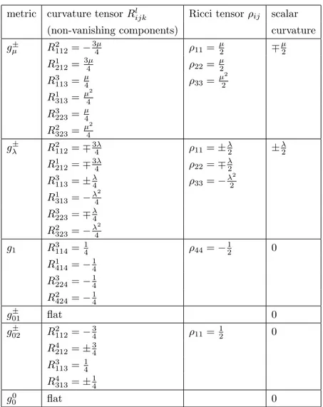
2.2. Case of group H3×R. See Table 2.
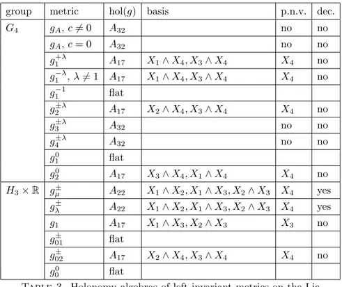
2.3. Holonomy. Now we calculate holonomy algebras hol(g) of each metricgfrom Theorems 1.3 and 1.4. Note that, since the nilpotent Lie group is simply connected, the restricted holonomy groupHol0(N, g) coincides with the full holonomy group
metric curvature tensorRl
ijk Ricci tensorρij scalar
(non-vanishing components) curvature
gA R2112= 3a2
4 R
2
113=b2 ρ11=−ad2+c
2
2d −
(c22+ad)1
2d
R3
112=34bcd R 3 113=
3c2−ad2
4d ρ22=− a1
2
R4112=d
−3b2
4d R
4 113=
−bc
d ρ23=−
b1
2
R1 212=−
3a1
4 R1213=−b1 ρ33=
(a2d2−c(d−b2))1
2d
R1
312=−b1 R1313=
(a2d2−c(3d−b2))1
4d ρ34=
b(ad2+c2)
2d
R1 412=−
c1
4 R
1 413=
b(ad2+c2)1
4d ρ44=
(b2d2+c3)1
2d
R2114= c2
4 R
3 223=−
a1
4
R3 114=−
b2
4 R
2 323=
a2 12
4
R4 114=−c
2
4d R
3 323=
b(b2−d)1
4d
R1 214=−
c1
4 R
4 323=
a(b2−d)1
4d
R1 314=
b(ad2+c2)1
4d R 2 423=
ab12
4
R1 414=
(b2d2+c3)1
4d R 3 423=
c(b2−d)1
4d R3 234= c1 4 R 4 423=
b(d−b2)1
4d
R4 234=−
b1
2 R
3 224=−
b1
4
R2 334=
(b2−d)12
4 R
2 324=
ab 412
R3 334=
bc21
4d R
3 324=
b2c1
4d
R4 334=−
ac21
4d R
4 324=−
abc1
4d
R2434= bc12
4 R
2 424=
b212
4
R3 434=
c3 1
4d R4424= bc2
1
4d
R4 434=−
bc2 1
4d R
4 424=−
b2c 1
4d
g1±λ R4 121=
(λ±1)(3λ∓1)
4λ R
3 223=
(λ±1)2
4λ ρ22= λ2−1
2λ 0
R1 212=
(λ±1)(3λ∓1)
4λ R
4 323=
∓(λ±1)2 4
g2±λ R2112=−34λ R 3
113=λ4 ρ11= λ
2 0
R4 212=∓
3λ
4 R
4 313=∓
λ2 4
g3±λ R4112=12 R
2
114=−λ2 ρ13=± λ
2 ±
λ 2
R3
412=∓λ2 R3214=∓λ2 ρ44=− λ2
2
R1 113=±
λ
4 R
4 134=±
λ 4
R3 313=∓
λ
4 R
3 434=−
λ2
4
g4±λ R2 113=±
3λ
4 R
2 224=−
λ
2 ρ24=− λ 2 0 R1 313= 3λ 4 R 3 324= λ
2 ρ33=
λ 2
R4 223=∓
1 2 R 4 334= λ 4 R3
423=λ2 R 2 434=∓λ
2
4
g0
1 flat 0
g0
2 R4112= 1 R4123=− 1
4 ρ22=− 1
2 0
R1 212=−
1 4 R 3 223= 1 4 R3
212=−1 R4312= 1 4
metric curvature tensorRl
ijk Ricci tensorρij scalar
(non-vanishing components) curvature
gµ± R2112=− 3µ
4 ρ11=
µ
2 ∓
µ 2
R1 212=
3µ
4 ρ22=
µ 2
R3 113=
µ
4 ρ33= µ
2 2
R1313= µ2
4
R3 223=
µ 4
R2 323=
µ2 4
gλ± R2 112=∓
3λ
4 ρ11=±
λ
2 ±
λ 2
R1
212=∓3λ4 ρ22=∓
λ 2
R3113=±λ
4 ρ33=−
λ2 2
R1 313=−
λ2 4
R3
223=∓λ4
R2323=−λ 2 4
g1 R3114= 14 ρ44=−
1
2 0
R1 414=−
1 4
R3 224=−
1 4
R2
424=−14
g01± flat 0
g02± R2
112=−34 ρ11=
1
2 0
R4212=±34
R3 113=
1 4
R4 313=±
1 4
g0
0 flat 0
Table 2. Curvature of left invariant metrics on the Lie group H3×R
We know that the holonomy algebra is a subalgebra of an isometry algebra, i.e. hol(g)≤o(2,2). According to the Ambrose–Singer theorem the algebra hol(g) is generated by the curvature operators R(Xi, Xj) and their covariant derivatives of
any order. Since the covariant derivatives and the curvature operators are known, we use the formula
(∇XmR(Xk, Xl))(Xj) =∇Xm(R(Xk, Xl)(Xj))−R(Xk, Xl)(∇XmXj)
to calculate the derivative∇XmR(Xk, Xl) of the curvature operator. Higher order
group metric hol(g) basis p.n.v. dec.
G4 gA, c6= 0 A32 no no
gA, c= 0 A32 no no
g1+λ A17 X1∧X4, X3∧X4 X4 no
g1−λ, λ6= 1 A17 X1∧X4, X3∧X4 X4 no
g1−1 flat
g2±λ A17 X2∧X4, X3∧X4 X4 no
g3±λ A32 no no
g4±λ A32 no no
g10 flat
g0
2 A17 X3∧X4, X1∧X4 X4 no
H3×R gµ± A22 X1∧X2, X1∧X3, X2∧X3 X4 yes
gλ± A22 X1∧X2, X1∧X3, X2∧X3 X4 yes
g1 A17 X1∧X3, X2∧X3 X3 no
g01± flat
g02± A17 X2∧X4, X3∧X4 X4 no
g00 flat
Table 3. Holonomy algebras of left invariant metrics on the Lie groups G4 andH3×R. (p.n.v.: parallel null vector; dec.: decom-posable.)
For the classification of holonomy algebras, we used the notation proposed by Ghanam and Thompson in [17]. Note that the results obtained in [17] were later improved by Galaev and Leistner in [16].
From the three algebras listed in the previous table only the full holonomy alge-braA32is irreducible and therefore the corresponding metrics are indecomposable.
Let us examine the geometric structure for the other two algebras.
In the case of the algebra A17 we have an invariant 2-dimensional null
distri-bution containing a parallel null vector field. Since the holonomy algebraA17 is
2-dimensional, according to [37], all projectively equivalent metrics are also affinely equivalent.
By the results of de Rham [13] and Wu [40], A22 corresponds to the product
of an irreducible 3-dimensional Lorentzian metric and a 1-dimensional flat factor adjusted so as to obtain a neutral signature. It is easy to check thatA22is spanned
byX1∧X2, X1∧X3, X2∧X3, corresponding to the subalgebra 3(c) from [37]. In
the same paper projective equivalence of the metricgof this type was investigated under some strict assumptions on the range of the curvature mapR: Λ2T
pN →
Λ2T
2.4. Walker metrics. We can observe that Walker metrics appear as the under-lying structure of neutral signature metrics on the nilpotent Lie groups with the holonomy algebraA17. It is a well known fact that metrics on the 2-step nilpotent
Lie groups with degenerate center admit Walker metrics. Additionally, we find an example of this kind of metric with non-degenerate center. Interestingly, a metric on a 3-step nilpotent Lie group with degenerate center is not necessarily a Walker one. For example, a family of metricsgA withc= 0 has degenerate center, but it
is not Walker.
Let us recall that there exist local coordinates (x, y, z, w) such that a Walker metric, with respect to the frame{ ∂
∂x, ∂ ∂y,
∂ ∂z,
∂
∂w}, has the form
0 0 1 0
0 0 0 1
1 0 a c
0 1 c b
, (4)
wherea,b andcare smooth functions.
In [36] Walker described an algorithm for finding appropriate local coordinates. LetDbe a 2-dimensional null distribution. Since the space is 4-dimensional, we haveD=D⊥. There exist local coordinates (x
1, x2, x3, x4) such thatDis spanned
by{ ∂ ∂x1,
∂
∂x2}. SinceDis totally null, we have
g ∂
∂x1
, ∂ ∂x2
= 0.
Now, we consider the vector fields{ξi}, i∈ {1,2} defined by
g(ξi, X) =dxi+2(X).
It follows that {ξi}2i=1 are orthogonal to any X ∈ D⊥ and hence they lie in D.
Moreover, they are linearly independent. Thus we can take
∂ ∂x =ξ
j 1
∂ ∂xj
, ∂
∂y =ξ
j 2
∂ ∂xj
, ∂
∂z = ∂ ∂x3
, ∂
∂w = ∂ ∂x4
, j∈ {1, . . . ,4}
to be our new coordinate frame.
Furthermore, it can be proven that, if a Walker metric possesses parallel vector field, there exist local coordinates such that functionsa,bandc do not depend on the variablex. Since the change of coordinates preserves the canonical form (4) of the metricg, it is easy to show that the coordinate transformations are given by
e x=∂z
∂ez x+ ∂z ∂we y+S
1(z, w),
e
z=α(z, w),
e y=∂w
∂ez x+ ∂w ∂we y+S
2
(z, w), we=β(z, w),
(see [3] for details).
group metric basis of null functions from
distribution Walker form
G4 g+λ1 X1−√1λX3, X4 a=a(y) =λ+11 y2
b=λ
c=c(y) =y g−λ1 , λ6= 1 X1−√1λX3, X4 a=a(y) =−λ−11 y2
b=−λ c=c(y) =y
g±λ2 X2+√1λX3, X4 a=a(y, z) =±λ1(y+z)2
b=±λ
c=c(y) =y g0
2 X3, X4 a=a(w) =±w2
b= 2 c=c(y) =y
H3×R g1 X1+X2, X3 a= 0
b=−1
c=c(y) =y g±02 X2+X3, X4 a=a(y) =∓y2
b=∓1 c=c(y) =y
Table 4. Walker form of metrics
Remark 2.6. Note that all of the Walker metrics from the Table 4 have zero scalar curvature. Hence, the components of the self-dual part of the Weyl tensor are given by
W11+=W13+ =W33+ =aww+ayy
b2
4 , W
+ 12=W
+ 22=W
+ 23= 0,
where indexes denote the partial derivatives. If the scalar curvature is zero, then the following holds (see[8]):
a) W+ vanishes if and only if W+ 11=W
+ 12= 0,
b) W+ is 2-step nilpotent operator if and only if W11+ 6= 0, W12+= 0,
c) W+ is 3-step nilpotent operator if and only if W+ 126= 0.
We can observe that all of our Walker metrics have 2-step nilpotent operatorW+, except the metricg1 which is previously shown to be conformally flat.
Remark 2.7. If we consider the action of the curvature map R on Λ2T pN =
Λ+⊕Λ− as in (3), with the standard identification
B=
0 B
B∗ 0
,
we conclude that our metric g0
2 on the Lie group G4 satisfies conditions W− =
0, B2
Λ− = 0 (here Λ− is the bundle of anti-self-dual bivectors) and the scalar curvature is constant. Metrics with these properties are studied in [5].
Lemma 2.1. On the4-dimensional nilpotent Lie groupN, all left invariant Walker metrics are geodesically complete.
Proof. All left invariant metrics on H3×R are geodesically complete (see [18]), therefore we have to prove the statement only for the metrics on the Lie groupG4.
Letγ(t) = (x1(t), x2(t), x3(t), x4(t)) be a geodesic curve on (G4, g) withγ(0) =
(x01, x02, x03, x04) and ˙γ(0) = ( ˙x10,x˙02,x˙03,x˙04).
The Lagrangian associated with the metricg has the form:
L(t) =bx˙4(t)2+ ˙x3(t) (2 ˙x1(t) +ax˙3(t)) + 2 ˙x4(t) ( ˙x2(t) +x2(t) ˙x3(t)).
Herea=a(x2, x3, x4) andbis constant. From the Euler–Lagrange equations:
d dt
∂L
∂x˙k
− ∂L
∂xk
= 0, k= 1, . . . ,4,
we get the following system of partial differential equations:
¨ x3= 0,
2 ˙x3x˙4−2¨x4+ax2x˙ 2 3= 0,
2 (x2x¨4+ ¨x1+ ˙x2x˙4+ax4x˙3x˙4) + ˙x3(ax3x˙3+ 2ax2x˙2) = 0, −2 ( ˙x2x˙3+b¨x4+ ¨x2) +ax4x˙
2 3= 0.
A standard but long calculation leads to the conclusion that all geodesics exist for
every t∈R.
3. Projective equivalence
In this section we look for metrics on the nilpotent Lie groups H3×RandG4
that are geodesically equivalent to the left invariant metrics from Theorems 1.3 and 1.4.
We say that the metricsg and ¯g aregeodesically equivalent if every geodesic of g is a (reparameterized) geodesic of ¯g. We say that they are affinely equivalent
if their Levi-Civita connections coincide. We call a metric g geodesically rigid if every metric ¯g, geodesically equivalent tog, is proportional tog. Weyl [39] proved that two conformally and geodesically equivalent metrics are proportional with a constant coefficient of proportionality.
The two connections∇={Γi
jk}and ¯∇={Γ¯ijk}have the same unparameterized
geodesics, if and only if their difference is a pure trace: there exists a (0,1)-tensor φsuch that
¯
For a parameterized geodesic γ(τ) of ¯∇, the curve γ(τ(t)) is a parameterized geodesic of∇if and only if the parameter transformationτ(t) satisfies the following ODE:
φαγ˙α=
1 2
d dt
log
dτ dt
,
where the velocity vector ofγwith respect to the parametertis denoted by ˙γ. Suppose that ∇ and ¯∇, related by (5), are the Levi-Civita connections of the metrics g and ¯g, respectively. Contracting (5) with respect to i andj, we obtain ¯
Γα
αi= Γααi+ (n+ 1)φi. From the other side, for the Levi-Civita connection∇ of a
metricg, we have Γα αk=
1 2
∂log|det(g)| ∂xk . Thus,
φi=
1 2(n+ 1)
∂ ∂xi
log
det(¯g) det(g)
=φ,i
for the functionφ:M −→Rgiven by
φ:= 1
2(n+ 1)log
det(¯g) det(g)
. (6)
The formula (5) implies that g and ¯g are geodesically equivalent if and only if for the functionφ, given by (6), the following holds:
¯
gij;k−2¯gijφk−g¯ikφj−¯gjkφi= 0, (7)
where “semi-colon” denotes the covariant derivative with respect to the connec-tion∇.
Consider the projective Weyl tensor
Wjkli :=Rjkli −
1 n−1 δ
i
lRjk−δkiRjl
,
whereRijklandRjkare components of the curvature and the Ricci tensor of
mani-fold (Mn, g). Weyl has shown [38] that the projective Weyl tensor does not depend on the choice of a connection within the projective class. Note that the converse is not true (see [21]).
In order to find the projective class of our 4-dimensional metrics, we use the formula
−2ga(iWaklj) =gabWab[l(i δj)k], (8) proposed by Matveev in [28], where the brackets “[ ]” denote the skew-symmetri-zation without division, and the brackets “( )” denote the symmetriskew-symmetri-zation without division.
Every metricggeodesically equivalent to ¯g has the same projective Weyl tensor as ¯g. We view the equation (8) as the system of homogeneous linear equations on the components of g; every metric g geodesically equivalent to ¯g satisfies this system of equations (8).
General algorithm:
In order to find all metrics ¯g that are projectively equivalent to g we first look for the solutions of the homogeneous system of the equations (8). The condition (8) is necessary but not sufficient, so we call such metrics candidates. Then, we check if each candidate satisfies the condition (7) which is sufficient for projective equivalence. If all candidates satisfying condition (7) are proportional to g, by a result of Weyl [39] the metric g is geodesically rigid. If the function φ satisfying relations (7) is constant, then ¯g is affinely equivalent tog.
Remark 3.1. Although the proposed algorithm was presented in [28] considering only the Lorentzian metrics, it is also valid for the metrics of arbitrary signature. Note that, by computing the candidates, we find all the possible pairs of geodesically equivalent metrics, regardless of their signature.
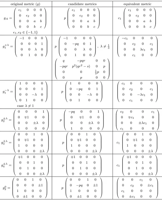
Applying the proposed algorithm, in a similar manner as in the case of Lorentz signature (see [7]) we can prove the following two theorems.
Theorem 3.1. Let g andg¯be geodesically equivalent metrics on the Lie groupG4 and letg be non-flat, left invariant. Then the following two possibilities hold:
a) If g is of typeg1±λ, g±λ2 , org0
2, then g and ¯g are affinely equivalent. The family of metrics g¯is 2-dimensional. Every metric ¯g is left invariant and of neutral signature.
b) Ifgis of typegA,g±λ3 org ±λ
4 , then it is geodesically rigid, i.e. g¯=cg, c∈
R.
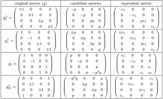
Note: In Table 5 we denote by c1, c2 ∈ R, c1 6= 0 constants and by p, q, r, s ∈
C∞(G4) functions on the Lie group.
Theorem 3.2. Let g and g¯ be geodesically equivalent metrics on the Lie group
H3×R, with g non-flat, left invariant. Then ¯g is affinely equivalent to g and left
invariant. The family of metrics ¯g is2-dimensional.
Note: In Table 6, we denote by c1, c2, c3∈R, c1, c36= 0 constants, and by p, q∈
C∞(H3×R) functions on the Lie group.
Remark 3.2. Note that if a metric g is flat and g andg¯ are geodesically equiva-lent, then their Levi-Civita connections coincide (moreover, they are equal to zero). Therefore, flat metrics were excluded from our calculations.
Our results, together with the known facts for the Riemannian and Lorentz case, give rise to the following, more general statement:
Theorem 3.3. Letg be a left invariant metric on the4-dimensional nilpotent Lie group. Ifgand¯gare geodesically equivalent, then they are either affinely equivalent or g is geodesically rigid. The metric ¯g is also left invariant, but not necessarily the same signature asg.
4. Isometry groups
Let us denote byI(N) the isometry group ofN. Set O(N) =Aut(N)∩I(N) and letIaut(N) =O(N)
original metric (g) candidate metrics equivalent metric
gA=
1 0 0 0
0 2 0 0
0 0 a b
0 0 b c
p
1 0 0 0
0 2 0 0
0 0 a b
0 0 b c
c1
1 0 0 0
0 2 0 0
0 0 a b
0 0 b c
1, 2∈ {−1,1}
g1+λ=
−1 0 0 0
0 0 0 1
0 0 λ 0
0 1 0 0
p
−1 0 0 0
0 −pq 0 1
0 0 λ 0
0 1 0 0
, λ6=13
−c1 0 0 0
0 c2 0 c1
0 0 λc1 0
0 c1 0 0
q −pqr 0 0
−pqr p2(qr2−s) 0 p
0 0 13p 0
0 p 0 0
g−1λ=
1 0 0 0
0 0 0 1
0 0 −λ 0
0 1 0 0
p
1 0 0 0
0 −pq 0 1
0 0 −λ 0
0 1 0 0
c1 0 0 0
0 c2 0 c1
0 0 −λc1 0
0 c1 0 0
caseλ6= 1
g2±λ=
0 0 0 1
0 ∓1 0 0
0 0 ±λ 0
1 0 0 0
p
−pq 0 0 1
0 ∓1 0 0
0 0 ±λ 0
1 0 0 0
c2 0 0 c1
0 ∓c1 0 0
0 0 ±λc1 0
c1 0 0 0
g3±λ=
0 0 1 0
0 ∓1 0 0
1 0 0 0
0 0 0 ±λ
p
0 0 1 0
0 ∓1 0 0
1 0 0 0
0 0 0 ±λ
c1
0 0 1 0
0 ∓1 0 0
1 0 0 0
0 0 0 ±λ
g4±λ=
∓1 0 0 0
0 0 1 0
0 1 0 0
0 0 0 ±λ
p
∓1 0 0 0
0 0 1 0
0 1 0 0
0 0 0 ±λ
c1
∓1 0 0 0
0 0 1 0
0 1 0 0
0 0 0 ±λ
g0 2 =
0 0 1 0
0 0 0 ±1
1 0 0 0
0 ±1 0 0 p
0 0 1 0
0 −pq 0 ±1
1 0 0 0
0 ±1 0 0
0 0 c1 0
0 c2 0 ±c1
c1 0 0 0
0 ±c1 0 0
original metric (g) candidate metrics equivalent metric
gµ±=
∓1 0 0 0
0 ∓1 0 0 0 0 ±µ 0 0 0 0 ±1
−p 0 0 0 0 −p 0 0 0 0 µp 0 0 0 0 q
−c1 0 0 0
0 −c1 0 0
0 0 µc1 0
0 0 0 c3
g±λ =
1 0 0 0
0 −1 0 0 0 0 ±λ 0 0 0 0 ∓1
±p 0 0 0 0 ∓p 0 0 0 0 λp 0 0 0 0 q
±c1 0 0 0
0 ∓c1 0 0
0 0 λc1 0
0 0 0 c3
g1=
1 0 0 0 0 −1 0 0 0 0 0 1 0 0 1 0
p 0 0 0 0 −p 0 0 0 0 0 p
0 0 p −p2q
c1 0 0 0
0 −c1 0 0
0 0 0 c1
0 0 c1 c2
g±02=
0 0 0 1 0 ±1 0 0 0 0 ∓1 0 1 0 0 0
−p2q 0 0 p
0 ±p 0 0 0 0 ∓p 0
p 0 0 0
c2 0 0 c1
0 ±c1 0 0
0 0 ∓c1 0 c1 0 0 0
Table 6. Projectively equivalent metrics on the Lie groupH3×R
letO(N) be the subgroup ofe I(N) that fixes the identity element ofN, then the following holds:
I(N) =O(N)e ·N. (9)
LetM be a pseudo-Riemannian manifold and letgbe the corresponding pseudo-Riemannian metric. A vector fieldX onM is called a Killing vector field if
g(∇VX, W) +g(V,∇WX) = 0 (10)
holds for any vector fieldsW andV onM.
All left invariant pseudo-Riemannian metrics onH3×Rare geodesically complete (see [18]), thus the set of all Killing fields is the Lie algebra of the full isometry group. Also, the 1-parameter groups of isometries constituting the flow of any Killing field are global. Therefore isometries produced by integration of Killing fields onH3×R are global. It is important to notice that not all metrics on the Lie groupG4 are complete.
Theorem 4.1. a) If the center of the Lie groupG4 is non-degenerate, thenO(Ge 4) is discrete and the isometry groupI(G4)of the corresponding metric is given by
b) In the case of the metrics gµ± and g±λ on the Lie group H3×R the isometry
group is given byI(H3×R) =O(He 3×R)n(H3×R), where
e
O(H3×R) =
cost −sint 0 0 sint cost 0 0
0 0 0
0 0 0 ¯
t∈R, ,¯∈ {−1,1}
, forgµ±,
e
O(H3×R) =
cosht sinht 0 0 sinht cosht 0 0
0 0 0
0 0 0 ¯
t∈R, ,¯∈ {−1,1}
, forgλ±.
c) In the case of the metric g1 on the group H3×R, the isometry group is given
byO(He 3×R)·(H3×R), where O(He 3×R)is a3-dimensional Lie group with the
corresponding Lie algebra defined by the structure equations
[ξ1, ξ2] =ξ2, [ξ1, ξ3] = 0, [ξ2, ξ3] = 0. (11)
Proof. (a) After solving the Killing equation (10), we observe that the algebra of isometries is generated only by the left translations. The group of isometries fixing the identity coincides with the group of isometric automorphisms, therefore the proposition holds.
(b) A direct calculation shows that the algebra of Killing vector fields is 5-dimensional. Also,H3×Ris a normal subgroup ofI(H3×R), thus in (9) we have the semi-direct product.
(c) Since ∇R ≡0, the metricg1 makes the simply connected groupH3×R a symmetric space. The group of isometries fixing the identity is identified with the group of linear isomorphisms ofh3⊕Rpreserving the curvature tensor. This shows that the isotropy of the identity insideI(H3×R) has dimension three, soI(H3×R) has at least seven linearly independent Killing vector fields.
Also, note that g1 is the only Walker metric corresponding to non-degenerate
center. We can change basis in such a way that the metricg1has the form presented
in Table 4.
By solving the Killing equation (10), we obtain exactly seven Killing vectors
{ξ1, . . . , ξ7} given by:
ξ1=−w 2
2 ∂
∂x+ (w−y) ∂ ∂y + 2
∂ ∂z+w
∂ ∂w, ξ
4=−e−z ∂
∂y,
ξ2=−w ∂ ∂x+
∂
∂y, ξ
5=
−ezy ∂ ∂x+
1 2e
z ∂
∂y+e
z ∂
∂w,
ξ3= ∂
∂z, ξ
6= ∂
∂x,
One can check that{ξ1, ξ2, ξ3} span the Lie algebra with the structure equations
(11). The remaining four vectors generate a Lie algebra defined by non-zero com-mutator [ξ4, ξ5] =ξ6, i.e. the Lie algebra h3⊕
R. The following relations are satisfied:
[ξ1, ξ4] =−ξ4, [ξ2, ξ4] = 0, [ξ3, ξ4] =−ξ4, [ξ1, ξ5] =ξ5, [ξ2, ξ5] = 0, [ξ3, ξ5] =ξ5, [ξ1, ξ6] = 0, [ξ2, ξ6] = 0, [ξ3, ξ6] = 0, [ξ1, ξ7] =−ξ2−ξ7, [ξ2, ξ7] =ξ6, [ξ3, ξ7] = 0. Since [ξ1, ξ7] = −ξ2−ξ7 6∈ L(ξ4, ξ5, ξ6, ξ7), H
3×Ris not a normal subgroup of I(H3×R).
On the other hand, an algebra generated by{ξ2, ξ4, ξ5, ξ6, ξ7}is a nilpotent Lie
algebra corresponding to the algebra L4
5 from the classification of Morozov [32]
or g5,1 from Magnin’s classification [27]. Therefore, the algebra of isometries is
isomorphic toR2ng5,1.
Remark 4.1. If we consider the metricgA on the Lie groupG4 whenc= 0, i.e. in the case of degenerate center, but a non-degenerate commutator subalgebra, we get that the isometry group is the same as in a non-degenerate case.
Example 1. Metricsg±01andg0
0 on the Lie groupH3×Rand metricsg10andg −λ 1
(forλ= 1) on the Lie groupG4are flat. Thus, the isometry group isO(2,2)nN.
From the above considerations, we conclude that if the center is degenerate and the holonomy algebra isA17, the corresponding metrics are Walker metrics of the
specific form given in the Table 4. Since all Walker metrics on a 4-dimensional nilpotent Lie groupN are geodesically complete (see Lemma 2.1), the Lie algebra of the isometry group coincides with the Lie algebra of the Killing vector fields.
Example 2. First, let us consider the metric g±02 on the Lie groupH3×R. The algebra of Killing vector fields is 6-dimensional and given by
ξ1= ∓6w−3yz2 ∂
∂x ∓3z(z−2) ∂ ∂y+z
3 ∂
∂w, ξ
4= ∂
∂w,
ξ2=−2yz ∂
∂x∓2(z−1) ∂ ∂y +z
2 ∂
∂w, ξ
5= ∂
∂z,
ξ3=−y ∂ ∂x∓
∂ ∂y +z
∂
∂w, ξ
6= ∂
∂x.
The subalgebra spanned by vectors {ξ3, ξ4, ξ5, ξ6} is defined by the non-zero
commutator [ξ5, ξ3] =ξ4, thus it is isomorphic toh 3⊕R.
Two remaining vectors ξ1 and ξ2 span an algebra isomorphic to
R2 and they satisfy the following relations:
The algebra of isometries is nilpotent, containing the maximal abelian ideal of the third order. Thus, it corresponds to the algebra of type 21 from the classification
of Morozov [32] (see also [27]).
Things get more complicated if we consider Walker metrics on the Lie groupG4.
Example 3. First, let us consider the metric g0
2. The algebra of Killing vector
fields is spanned by
ξ1= ∂
∂z, ξ
4=∓(z+ 1)w ∂
∂x±z ∂ ∂y +
∂ ∂w,
ξ2= ∂
∂x, ξ
5=
−e−z ∂ ∂y,
ξ3=−w ∂ ∂x+
∂
∂y, ξ
6=−ez(y±w)∂
∂x −
1∓1
2
ez ∂ ∂y +e
z ∂
∂w.
It is an easy calculation to show that the algebra of isometries is solvable and it contains the maximal nilpotent ideal generated by vectors{ξ2, ξ3, ξ4, ξ5, ξ6}. This
ideal is isomorphic tog5,4, therefore we observe that the algebra of isometries is
isomorphic tog6,84(from the the classification of Mubarakzjanov [33]).
Example 4. In the case of the metric g±λ2 , the Killing vectors have the form ξ1=
∓6λw−3yz2+3 4z
4−2z3
∂
∂x ∓3λz(z−2) ∂ ∂y +z
3 ∂
∂w,
ξ2=1
3z −6y+ 2z
2
−3z ∂
∂x ∓2λ(z−1) ∂ ∂y+z
2 ∂
∂w,
ξ3=
−y+1 2z
2
∂
∂x ∓λ ∂ ∂y +z
∂ ∂w,
ξ4= ∂ ∂w, ξ
5=w ∂
∂x − ∂ ∂y+
∂ ∂z, ξ
6= ∂
∂x.
Thus the algebra of isometries is 6-dimensional and the subalgebra spanned by
{ξ3, ξ4, ξ5, ξ6}is 3-step nilpotent.
After an appropriate change of basis vectors, we can see that the algebra of
isometries is exactly the algebra from Example 2.
Example 5. Finally, we discuss the metricsg1+λ andg1−λ (forλ6= 1).
For convenience, setµ= 1±λ1 . Note that 0< µ <1 for everyλ >0 in the case of the metricg+λ1 , while in the case ofg1−λ two possibilities may occur: µ >1 for 0< λ <1 andµ <0 forλ >1.
After a long but straightforward calculation, we obtain 6-dimensional algebras of Killing vector fields:
ξ3= (w−y) ∂ ∂x−
1 µ
∂ ∂y+z
∂
∂w, ξ
5= ∂
∂w,
ξ4= ∂
∂x, ξ
6= ∂
where
ξ1=ez
√ µ
−y√µ ∂ ∂x+
µ−√µ µ
∂ ∂y +
∂ ∂w
,
ξ2=e−z√µ
y√µ ∂ ∂x+
µ+√µ
µ ∂ ∂y +
∂ ∂w
,
whenµ >0, and
ξ1=µysin(z√−µ) ∂
∂x + (sin(z
√
−µ)−√−µcos(z√−µ)) ∂ ∂y
−√−µcos(z√−µ) ∂ ∂w,
ξ2=−µycos(z√−µ) ∂
∂x −(cos(z
√
−µ) +√−µsin(z√−µ))∂ ∂y
−√−µsin(z√−µ) ∂ ∂w, whenµ <0.
In both cases{ξ3, ξ4, ξ5, ξ6}generate the algebra of left translations and{ξ1, ξ2}
form an algebra isomorphic toR2.
The algebra of Killing vector fields for g1+λ and g1−λ (for λ 6= 1) is solvable, containing the maximal nilpotent ideal of dimension five and it is isomorphic to
the algebrag6,84 (see [33]).
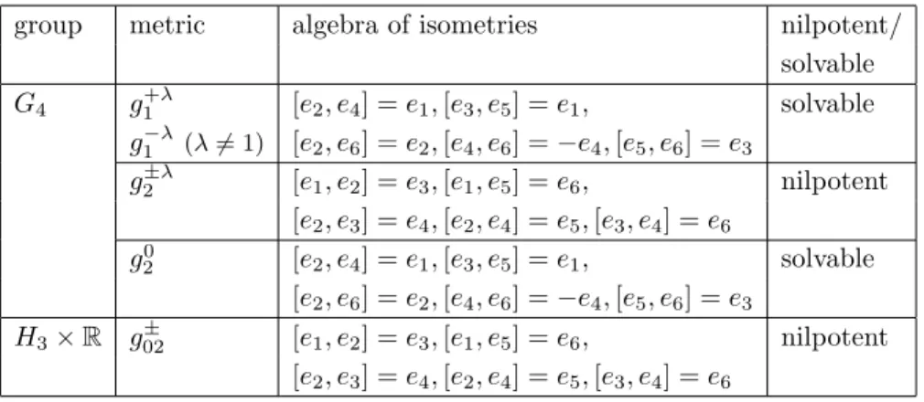
The preceding examples and Remark 4.1 directly imply:
Lemma 4.1. (a) If the center of the Lie group H3×R is degenerate and H3×
R is non-flat, then the corresponding algebra of isometries is 6-dimensional and
isomorphic to the algebra listed in the table below.
(b) If the Lie groupG4is non-flat with degenerate center, then the corresponding algebra of isometries is either 4-dimensional, generated by the left translations (in the case ofgA,c= 0) or it is6-dimensional and isomorphic to one of the algebras presented in Table 7.
Corollary 4.1. For any left invariant metric the following inequality holds:
dimI(H3×R)>dim(H3×R).
This does not hold for the Lie group G4.
Corollary 4.2. If the center of a4-dimensional nilpotent Lie groupNis degenerate and N is non-flat, then dimO(Ne )≤2. The equality holds for all metrics except the metricgA (forc= 0) on the Lie groupG4, when O(Ne )is discrete.
Acknowledgment
group metric algebra of isometries nilpotent/ solvable
G4 g+λ1 [e2, e4] =e1,[e3, e5] =e1, solvable
g−λ1 (λ6= 1) [e2, e6] =e2,[e4, e6] =−e4,[e5, e6] =e3
g±λ2 [e1, e2] =e3,[e1, e5] =e6, nilpotent
[e2, e3] =e4,[e2, e4] =e5,[e3, e4] =e6
g0
2 [e2, e4] =e1,[e3, e5] =e1, solvable
[e2, e6] =e2,[e4, e6] =−e4,[e5, e6] =e3
H3×R g±02 [e1, e2] =e3,[e1, e5] =e6, nilpotent
[e2, e3] =e4,[e2, e4] =e5,[e3, e4] =e6
Table 7. Isometry algebras for Walker metrics
References
[1] S. Azimpour, M. Chaichi, M. Toomanian,A note on4-dimensional locally conformally flat Walker manifolds, J. Contemp. Math. Anal. 42 (2007), 270–277. MR 2416714.
[2] V.V. Balashchenko, Yu. G. Nikonorov, E. D. Rodionov, V. V. Slavsky,Homogeneous spaces: theory and applications: monograph(in Russian), Polygrafist, Hanty-Mansijsk, 2008.http: //elib.bsu.by/handle/123456789/9818
[3] A. Bejancu, H. R. Farran,Foliations and geometric structures, Mathematics and Its Appli-cations (Springer), 580. Springer, Dordrecht, 2006. MR 2190039.
[4] E. Beltrami,Saggio di interpretazione della geometria non-euclidea, Giornale di Matematiche VI (1868).
[5] D. E. Blair, J. Davidov, O. Muˇskarov,Isotropic K¨ahler hyperbolic twistor spaces, J. Geom. Phys. 52, (2004), 74–88. MR 2085664.
[6] N. Blaˇzi´c, S. Vukmirovi´c,Four-dimensional Lie algebras with a para-hypercomplex structure, Rocky Mountain J. Math. 40 (2010), 1391–1439. MR 2737373.
[7] N. Bokan, T. ˇSukilovi´c, S. Vukmirovi´c, Lorentz geometry of 4-dimensional nilpotent Lie groups, Geom. Dedicata 177 (2015), 83–102. MR 3370025.
[8] M. Brozos-V´azquez, E. Garc´ıa-R´ıo, P. Gilkey, S. Nikˇcevi´c, R. V´azquez-Lorenzo,The geometry of Walker manifolds, Synthesis Lectures on Mathematics and Statistics. Morgan & Claypool Publishers, Williston, VT, 2009. MR 2656431.
[9] M. Chaichi, E. Garc´ıa-R´ıo, Y. Matsushita,Curvature properties of four-dimensional Walker metrics, Classical Quantum Gravity 22 (2005), 559–577. MR 2115361.
[10] L. A. Cordero, P. E. Parker, Left-invariant Lorentz metrics on3-dimensional Lie groups, Rend. Mat. Appl. (7) 17 (1997), 129–155. MR 1459412.
[11] L. A. Cordero, P. E. Parker, Isometry groups of pseudoriemannian 2-step nilpotent Lie groups, Houston J. Math. 35 (2009), 49–72. MR 2491866.
[12] V. del Barco, G. P. Ovando,Isometric actions on pseudo-Riemannian nilmanifolds, Ann. Global Anal. Geom. 45 (2014), 95–110. MR 3165476.
[13] G. de Rham,Sur la r´eductibilit´e d’un espace de Riemann, Comment. Math. Helv. 26 (1952), 328–344. MR 0052177.
[15] M. Fern´andez, M. J. Gotay, A. Gray, Compact parallelizable four-dimensional symplectic and complex manifolds, Proc. Amer. Math. Soc. 103 (1988), 1209–1212. MR 0955011. [16] A. Galaev, T. Leistner,Recent developments in pseudo-Riemannian holonomy theory,
Hand-book of pseudo-Riemannian geometry and supersymmetry, 581–627, IRMA Lect. Math. Theor. Phys., 16, Eur. Math. Soc., Z¨urich, 2010. MR 2681602.
[17] R. Ghanam, G. Thompson,The holonomy Lie algebras of neutral metrics in dimension four, J. Math. Phys. 42 (2001), 2266–2284. MR 1825956.
[18] M. Guediri,Sur la compl´etude des pseudo-m´etriques invariantes `a gauche sur les groupes de Lie nilpotents, Rend. Sem. Mat. Univ. Politec. Torino 52 (1994), 371–376. MR 1345607. [19] G. S. Hall, D. P. Lonie, Projective structure and holonomy in four-dimensional Lorentz
manifolds, J. Geom. Phys. 61 (2011), 381–399. MR 2746125.
[20] G. S. Hall, Z. Wang,Projective structure in4-dimensional manifolds with positive definite metrics, J. Geom. Phys. 62 (2012), 449–463. MR 2864491.
[21] G. S. Hall,On the converse of Weyl’s conformal and projective theorems, Publ. Inst. Math. (Beograd) (N.S.) 94(108) (2013), 55–65. MR 3137490.
[22] Sz. Homolya, O. Kowalski,Simply connected two-step homogeneous nilmanifolds of dimen-sion 5, Note Mat. 26 (2006), 69–77. MR 2267683.
[23] A. Kaplan, Riemannian nilmanifolds attached to Clifford modules, Geom. Dedicata 11 (1981), 127–136. MR 0621376.
[24] V. Kiosak, V.S. Matveev,Complete Einstein metrics are geodesically rigid, Comm. Math. Phys. 289 (2009), 383–400. MR 2504854.
[25] J. L. Lagrange, Sur la construction des cartes g´eographiques, Nouveaux m´emoires de l’Acad´emie royale des sciences et belles-lettres de Berlin, 1779.
[26] J. Lauret, Homogeneous nilmanifolds of dimensions 3 and 4, Geom. Dedicata 68 (1997), 145–155. MR 1484561.
[27] L. Magnin,Sur les alg`ebres de Lie nilpotentes de dimension ≤7, J. Geom. Phys. 3 (1986), 119–144. MR 0855573.
[28] V. Matveev,Geodesically equivalent metrics in general relativity, J. Geom. Phys. 62 (2012), 675–691. MR 2876790.
[29] J. Mikeˇs, I. Hinterleitner, V. Kiosak,On geodesic mappings of affine connection manifolds, Acta Physica Debrecina 42 (2008), 19–28.
[30] J. Mikeˇs, A. Vanˇzurov´a, I. Hinterleitner, Geodesic mappings and some generalizations, Palack´y University Olomouc, Faculty of Science, Olomouc, 2009. MR 2682926.
[31] J. Milnor,Curvatures of left invariant metrics on Lie groups, Advances in Math. 21 (1976), 293–329. MR 0425012.
[32] V. V. Morozov,Classification of nilpotent Lie algebras of sixth order(in Russian), Izv. Vysˇs. Uˇcebn. Zaved. Matematika (1958), no. 4 (5), 161–171. MR 0130326.
[33] G. M. Mubarakzjanov, Classification of solvable Lie algebras of sixth order with a non-nilpotent basis element (in Russian), Izv. Vysˇs. Uˇcebn. Zaved. Matematika (1963), no. 4 (35), 104–116. MR 0155872.
[34] S. Rahmani,M´etriques de Lorentz sur les groupes de Lie unimodulaires, de dimension trois, J. Geom. Phys. 9 (1992), 295–302. MR 1171140.
[35] N. S. Sinyukov,On geodesic mappings of Riemannian spaces onto symmetric Riemannian spaces(in Russian), Dokl. Akad. Nauk SSSR (N.S.) 98 (1954), 21–23. MR 0065994. [36] A. G. Walker,Canonical form for a Riemannian space with a parallel field of null planes,
[37] Z. Wang, G.S. Hall,Projective structure in4-dimensional manifolds with metric signature
(+,+,−,−), J. Geometry and Physics, (2013), 37–49. MR 3019271.
[38] H. Weyl,Zur Infinitesimalgeometrie: Einordnung der projektiven und der konformen Auf-fasung, Nachrichten von der Gesellschaft der Wissenschaften zu G¨ottingen, Mathematisch-Physikalische Klasse (1921), 99–112; reprinted in “Selecta Hermann Weyl”, Birkh¨auser Ver-lag, Basel und Stuttgart, 1956.
[39] H. Weyl, Geometrie und Physik, Die Naturwissenschaftler 19 (1931), 49–58; reprinted in “Gesammelte Abhandlungen”, Band III, Springer-Verlag, 1968.
[40] H. Wu, Holonomy groups of indefinite metrics, Pacific J. Math. 20 (1967), 351–392. MR 0212740.
T. ˇSukilovi´c
University of Belgrade, Faculty of Mathematics, Belgrade, Serbia [email protected]