Comparativa del algoritmo de K Means contra los mapas auto organizados en la clasificación de pacientes ortopédicos con problemas de columna vertebral

Texto completo

(1)Informatics in Medicine Unlocked 16 (2019) 100206. Contents lists available at ScienceDirect. Informatics in Medicine Unlocked journal homepage: www.elsevier.com/locate/imu. Comparison between K-means and Self-Organizing Maps algorithms used for diagnosis spinal column patients. T. Nicolas Andres Melo Riveros∗, Bayron Alexis Cardenas Espitia, Lilia Edith Aparicio Pico Electronic Engineering, Universidad Distrital Francisco José de Caldas, Colombia. A R T I C LE I N FO. A B S T R A C T. Keywords: Machine learning K-means Self-Organizing Maps Unsupervised learning Clustering Kappa coefficient Confusion matrix. Back pain is a problem that affects at least 90% of the human population during their lifetimes, and it is one of the main causes of absence from work. Despite the large number of medical cases, there is insufficient research in this field, due in part to the necessity of administering multiple medical exams to patients with vertebral problems for accurate diagnosis. In addition, the cause of back pain may be benign, and heal without treatment. In this study, two artificial intelligence algorithms were employed to classify patients with spinal problems. The algorithms used were K-means and Self Organizing Maps (SOM). With these techniques, two models were obtained that provided a generalization error of less than 10%. The models were compared based on metrics that enable the measurement of classifier performance, including the sensitivity, specificity, precision, and negative predictive value (NPV), as well as Cohen's Kappa index to evaluate concordance. It was found that the model trained with SOM outperformed the model trained with K-means, with improved detection of patients having vertebral problems. Additionally, it was found that the SOM and K-means models yielded similar precision as compared with models obtained with different algorithms reported elsewhere. The values yielded were in agreement with those of expert orthopedic physicians.. 1. Introduction The aim of machine learning is to develop computational techniques to learn and/or imitate human behavior. Machine learning seeks to develop programming that is able to generalize a specific behavior, starting from an information set, by providing example to the machine. The term “generalize” refers to the capacity to respond adequately to new information [1]. Some problems studied by this branch of biomedical science include classification problems, regression, and estimation. These problems are addressed by the perspectives of computational learning: either supervised learning or unsupervised learning. Supervised learning aims to find a function that satisfies the relationship between the input/output pairs. In this learning method, training is controlled by an external agent (supervisor) that provides the algorithm with the input characteristics, and alters the system depending on whether the answer obtained matches with the output tags [2]. Unsupervised learning is an automatic learning method; a model is adjusted to the observation of a set or data input. The difference versus supervised learning is that unsupervised learning does not consider prior knowledge; data is treated as random variables, and the aim is to find the probability density distribution that accommodates them [3].. ∗. Usually, the approach of unsupervised learning is given by grouping data with similar characteristics; this grouping process is known as clustering, which consists in separating each group with different characteristics in sets called clusters. The output of these models represent familiarity or similarity of the information presented at the input. These models have a memory capacity, learning capacity and pattern recognition capacity [4]. Diagnosing persons with lumbar problems is difficult because of the many different medical conditions that can exist. A large number of medical examinations are required to determine the problem that affects the patient. In this paper, two clustering techniques are proposed, which are the K-means algorithm and Self-Organizing Maps - as a more rapid mode to classify patients with vertebral column conditions. Generalization error measurement is needed to make a comparison between the two algorithms, which implies that output data is not used during training, but during validation. Furthermore, a statistical comparison is performed using derived metrics of the confusion matrix, and also contrasting the concordance degree of the models measured by the Cohen Kappa coefficient.. Corresponding author. E-mail addresses: namelor@correo.udistrital.edu.co, nicoamelo@hotmail.com (N.A. Melo Riveros), bacardenase@correo.udistrital.edu.co (B.A. Cardenas Espitia).. https://doi.org/10.1016/j.imu.2019.100206 Received 9 May 2019; Received in revised form 9 July 2019; Accepted 11 July 2019 Available online 12 July 2019 2352-9148/ © 2019 Published by Elsevier Ltd. This is an open access article under the CC BY-NC-ND license (http://creativecommons.org/licenses/BY-NC-ND/4.0/)..

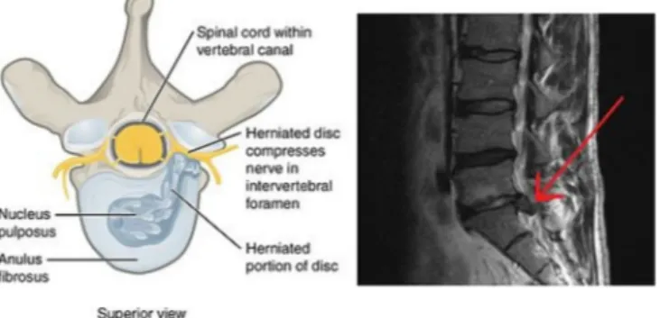
(2) Informatics in Medicine Unlocked 16 (2019) 100206. N.A. Melo Riveros, et al.. Fig. 1. (a) Illustration of herniated spinal disc, superior view. (b) MRI showing herniated L5-S1 disc (red arrow tip), sagittal view.. 2. Theoretical framework 2.1. Spine orthopedic problems Back pain is the most common reason for visits to the doctor worldwide. However, back pain research has not been a major concern in medicine, mainly because of a tendency to heal without extensive treatment. However, the principal cause of employee absenteeism is lumbar pain. It is estimated that at least 90% of human population will suffer from lumbar pain during their lifetime. The following are some spine orthopedic problems that bear some relevance for this article [5,6]: 1. Herniated disk: According to the clinical guides of the North American Spine Society (NASS), a herniated disk is the condition in which there is an intervertebral disk matter displacement; the disk matter protrudes from the normal margins of the intervertebral disk space. The causes of lumbar disk herniation is not entirely known, but is believed that the cause is mechanical and biological processes with a degenerative disk process that plays an important role [7,8] (Fig. 1). 2. Spondylolisthesis: Spondylolisthesis refers to the actual vertebra movement. This happens when the pars interarticularis separates and allows the vertebra to move out of its usual position, causing pain. Spondylolisthesis usually takes place between the fourth and fifth lumbar vertebrae, or between the last vertebra and the sacrum [9,10] (Fig. 2).. Fig. 2. A medical illustration depicting spondylolisthesis.. (the weights of the neurons). These parameters are often random, as well as the neural form arrangement. 2. Sample: in this stage, the map model receives an input vector at a time. Here, a x ∈ Rn vector is associated to an element in the SOM by a mi ∈ Rn parametric vector named model. The counterpart of an input vector in the SOM model is defined as the mc element that better connects with the input, which is determined by a Euclidean distance.. ||x − mc || = mín ||x − mi ||. 2.2. Self-Organizing Maps. (1). 3. Searching similarity between input patterns and neuron location: the idea of a learning process is that for each x input vector, the nearest node changes to be closer to x. 4. Update of neuronal weights based on distance: when the distance between the input vector and neuron is found, this is used to change the function parameters of the neuron according to the following equation:. Self-Organizing Maps (SOM) are a neural model inspired by biological systems and self-organization systems. They are used to classify information and reduce the variable number of complex problems. They allow visualization of information via a two-dimensional mapping [11]. Self-Organizing systems can change their internal structure and function in response to external stimuli, or by influence of elements from the same system. A SOM is a simple layer neural network with N neurons distributed in space in a grid mode. Most applications are displayed in a rectangular representation, although there are some hexagonal representations, or other shapes with more sides. These produce a low dimensional projection of a dataset distribution in a high dimension space [12]. In the SOM method, the learning process considers similarity between the input vector and distance between neurons. To do this, Euclidean methods are used, and it is also necessary to use correlation, directional cosine, and block distances. The algorithm to train the SOM can be summarized as follows [13]:. mi (t + 1) = mi (t ) + hci (t )[x (t ) − mi (t )]. (2). Where t ∈ N is the discreet time, mi ∈ Rn are the map weights, and hci (t ) is the vicinity function. 5. Repeat till convergence: steps 2, 3 and 4 are repeated until the SOM convergence leads to a stable map. To assure convergence and stability, the radius between the set of neurons and the learning rate must decrease in each iteration until reaching zero [14].. 1. Initialization: In this stage, the parameters of the SOM are initialized 2.

(3) Informatics in Medicine Unlocked 16 (2019) 100206. N.A. Melo Riveros, et al.. ● ai is the number of samples that belong to the Ci class. ● pj is the number of samples that the sorter classifies as pertaining to the Cj class. ● nij is the samples number of the Ci class that are classified as pertaining to Cj class. ● N is the total number of samples. 2.3. K-means algorithm K-means is an algorithm of data mining that utilizes clustering. As previously mentioned, the clustering technique consists of dividing a dataset into groups (clusters) with similar characteristics. Clustering uses unsupervised learning models; this means that the resultant clusters are not known before the grouping algorithm is implemented. Each cluster is an input dataset grouped around a central point or centroid which has a minimum distance as compared with other centroids of other clusters. The K-means algorithm uses an iterative ordained process to group the dataset. Wherein, the number of desired clusters and initial centroids are taken as input entries, and the final centroids are taken as output. If K clusters are required, then there will be K initial centroids and K final centroids. After finishing the K-means algorithm, each dataset object becomes a member of a cluster. This cluster is determined by seeking the most approximate characteristics between the cluster centroid and the object [15]. Among the clustering techniques, this is not a hierarchical type, as all sets are generated at the same level. The algorithm is summarized as [16]:. From this matrix, four proportions are calculated, which are useful in the analysis of sorters [20]: True positive (TP[Ci ]): The number of correct predictions where the pertaining Ci class data are classified as such.. FP (Ci ) =. ∑ xj ;. TN (Ci ) = 1 −. (4). (9). Specificity (Ci ) =. TN (Ci ) TN (Ci ) + FP (Ci ). (10). Precision: It expresses the probability that a prediction indicating that the data pertains to Ci class is true. 2. 11. :. 21. 12. :. :. :. :. :. Where:. (8). Specificity: It expresses the probability that the model classifies an observation not pertaining to Ci class as such.. Precision (Ci ) =. In classification problems, the accuracy degree of a sorter cannot be considered complete unless it has been evaluated. This accuracy degree shows the concordance between the classes assigned by the sorter and the respective classes of the training dataset that it takes as reference. A common mechanism used to evaluate the accuracy of a sorter is called confusion matrix or error and contingency matrix. This is an nxn matrix size (with n as the number of classes) with the form [18,19]:. 1. TP (Ci ) TP (Ci ) + FN (Ci ). Sensitivity (Ci ) =. 2.4. Confusion matrix. 2. pi − nii N − ai. 1≤j≤l. 5. Repeat steps 3 and 4 until convergence (until the number of changes in the centroids, or in the data belonging to a cluster, is zero or an N value determinate).. 1. (7). Using the true and false positive or negative rates, more elaborated metrics are calculated to analyze the behavior of the classifiers, which are (mentioning only those of interest in this article) [21]: Sensitivity: It expresses the probability that the model classifies an observation pertaining to Ci class as such.. With mj as the number of data that belongs to the jth cluster.. 1. pi − nii N − ai. True Negative (TN[Ci ]): The number of correct predictions where the not pertaining Ci class data are classified as such.. (3). i ∈ Cj. (6). False Positive (FP[Ci ]): The number of wrong predictions where the not pertaining Ci class data are classified as pertaining to that class.. 4. Recalculate the centroid vector using the average criteria:. 1 mj. nii ai. FN (Ci ) = 1 −. With x i as the ith sample of the training set and cj as the jth centroid.. C ∗j =. (5). False Negative (FN[Ci ]): The number of wrong predictions where the pertaining Ci class data are classified as not pertaining to that class.. 1 Clusters number selection (L) 2. Initialization of the centroids (Random or taking the L first training data like centroids) [17]. 3. Allocation of the training data to each cluster based on the minimum distance criterion.. ||x i − cj || = mín j ||x i − cj || ; 1 ≤ j ≤ l. nii ai. TP (Ci ) =. 22. 2. … … … : … : … …. … … … : :. : … : … …. TP (Ci ) TP (Ci ) + FP (Ci ). (11). Negative predictive value (NPV): It expresses the probability that a prediction indicating that the data doesn't pertain to Ci class is true. NPV (Ci ) =. TN (Ci ) TN (Ci ) + FN (Ci ). (12). 2.5. Kappa index. 1. The Kappa index (K) proposed by Jacob Cohen [22] is a measure of the existent concordance between the frequencies of occurrence of a class (Pe ) and the frequencies obtained for that class when the classifier is used (Po ). Mathematically it is defined as [23]:. 2. :. :. :. :. K=. Po − Pe 1 − Pe. (13). Where:. N. k. Po = 3. ∑i = 1 nii N. (14).

(4) Informatics in Medicine Unlocked 16 (2019) 100206. N.A. Melo Riveros, et al.. column [27]. The pelvic radius is the distance between the center of the pelvis and the S1 reference point of the column [28].. Table 1 Assessment scale of the Kappa index. Kappa (K). Concordance degree. < 0,00 0,00–0,20 0,21–0,40 0,41–0,60 0,61 -0,80. Without concordance Insignificant Average Moderate Substantial. 3. Methodology 3.1. General For both K-means and SOM, an equivalent experimentation process was carried out, exploring architectures from 3 to 10 clusters/neurons, to select the solution with the least generalization error among the achieved results. After finding these two solutions, the confusion matrix was calculated for the entire dataset, and from it, the true and false positive/negative rates of each model were calculated. With the latter, measures of sensitivity, specificity, precision, and NPV were determined to make a statistical comparison of the models. Moreover, using the data of the confusion matrices and applying equations (14) and (15), the frequencies Po and Pe were calculated, and successively with them the values of the Kappa indices were calculated to compare the concordance degree of the obtained models.. k. Pe =. ∑i = 1 ai⋅pi. (15). N2. Table 1 shows the assessment scale of the Kappa index (proposed by Landis and Koch) [24]: 2.6. Database The database used in this article was taken from the UCI Machine Learning Repository [25] and is titled “Vertebral Column Data Set”. The database comprises a biomedical dataset built by Dr. Henrique da Mota during his period of medical residency in the Group of Investigation Applied in Orthopedics (GARO) of the medical-surgical center of rehabilitation of Massues, Lyon (France). It has 310 samples, each one with 6 biomechanical characteristics derived from the pelvis orientation form and the lumbar column. The output labels or classes associated to each vector of characteristics are:. 3.2. K-means algorithm The K-means algorithm was programmed in MATLAB and 4 tests were executed. In each test the best results for architectures between 3 and 10 clusters were achieved (8 architectures for test). Three clusters were utilized as the minimum because the problem has 3 classes. Ten (10) clusters were set as the maximum because exploring 8 architectures was sufficient, and although increasing the complexity could give better results, the purpose of this study was to find the simplest solution. In every test, 1000 experiments were carried out, reorganizing randomly the database in each one of them, because the algorithm is a heuristic process. Eighty percent (80%) of the database was taken for the training process and the remaining 20% for validation. The experimental process consisted of initializing the centroids, taking the first L data and assigning them to the nearer cluster via the minimum distance criterion. Thereafter, the centroids were recalculated, and the data assigning process was repeated for each cluster, until the change of each data approached zero. When this convergence condition of the algorithm was fulfilled, the resultant model was taken, and the validation process was performed (with 20% of the data unknown by the model). If the validation error of the architecture was less than the validation error of the best architecture previously stored, the new validation error replaced the one previously stored. Finally, after making 1000 experiments per architecture, 8 solutions were found with the lowest error; which correspond to the 8 architectures from 3 to 10 clusters. Fig. 3 shows the flowchart that summarizes the experimentation process.. ● Patient with Disk hernia (DH) ● Patient with Spondylolisthesis (SL) ● Normal Patient (NO) It has 60 samples pertaining to class 1, 150 samples for class 2, and 100 samples for class 3. The input dataset was not subject to any processing while the linguistic labels of the output set are mapped in the next way: DH as class 1, SL as class 2 and NO as class 3. Table 2 shows the description of each input for the model, the range, and the output label description with the respective numerical allocation made. The input variables observed in Table 2 are biomedical variables that describe the pelvis and lumbar spine form and orientation. Whereas: pelvic incidence angle, known as IP, is the angle formed by the perpendicular line to the midpoint of the platform of the sacrum and the line connecting this point to the central axis of the femoral head. Pelvic inclination or pelvic edition angle defines the position of the pelvis in space. The sacral slope corresponds to the angle between the sacrum cymbal and the horizontal plane [26]. The lumbar lordosis angle allows measurement of the curvature that exists in the vertebral Table 2 Description of the input/output dataset of the orthopedic patients of the vertebral column classification problem. Input. Description. Range. X1 X2 X3 X4 X5 X6. Pelvic incidence Pelvic inclination Angle of lordosis lumbar Sacral slope Pelvic radius Degree of Spondylolisthesis. 26.15, 129.83 −6.55, 49.43 14.00, 125.74 13.37, 121.43 70.08, 163.07 −11.06, 418.54. Output. Description. Class. Y. Type of orthopedic patient of vertebral column. 3.3. Self-Organizing Maps During the experimental process with the SOM algorithm, the SOM toolbox included in MATLAB was used, and some parameters were altered. In the same way as K-means, architectures between 3 and 10 neurons were explored (using hexagonal grids) and in total 4 tests were executed. Hexagonal grids were used because this is the default value in the SOM toolbox, and varying this parameter involved exploring a greater number of solutions as compared to K-means. A thousand experiments were performed per every one of these architectures. In each one there was a random reorganization of the database, taking 80% for training and 20% for validation. This was necessary because if the same database were to be taken for training in the experiments, the error would be the same. In each experiment, the SOM was defined, the map weights were initialized, the neuronal network was trained with the train function,. - With Herniated Disk (DH) = 1 - Spondylolisthesis (SL) = 2 - Normal (NO) = 3. 4.

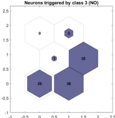
(5) Informatics in Medicine Unlocked 16 (2019) 100206. N.A. Melo Riveros, et al.. Fig. 3. Flowchart of the experimentation process with the K-means algorithm.. 739). With SOM algorithm, the same quantity of architectures as in Kmeans was explored. The grid values were between 3 and 10 neurons, which are equivalent to the clusters used in the first algorithm. Just as with K-means, the best solution yields an error of 4.839%. Table 4 displays the results of the solution set for the four tests and the grid size used (Hexagonal grids). The best solution obtained for the SOM algorithm was achieved with the architecture of 6 neurons (hexagonal grid of 2 × 3) in the experiment number 570 during the first test, and it presented a generalization error of 4.839%. The experiment number was obtained due to each experiment being enumerated with a reference. Fig. 7 illustrates the behavior of the generalization error for the set of solutions during test 1, where the minimum for 6 neurons is shown. Fig. 8 shows the error behavior for each experiment executed for the architecture of 6 neurons. Also, the experiment in which the best result for this architecture was achieved is highlighted (experiment number 570). In Figs. 9–11, the neurons activated for each data set are shown. These figures belong to the 2 × 3 SOM grid obtained in the first test (see Fig. 12). Fig. 11 shows the assignation of classes for each one neuron in the architecture of 6 neurons obtained with SOM. Tables 5 and 6 show the confusion matrices for the models obtained with K-Means (7 clusters) and SOM (2 × 3 grid), respectively. Table 7 shows the true and false positive/negative rates for each class, derived from the confusion matrix of each model: Table 8 shows the sensitivity, specificity, precision and NPV measurements of both models (from the data in Table 7). Table 9 shows the average measures of sensitivity, specificity, precision, and NPV of the three classes, for each of the models: Table 10 shows the Kappa index obtained by applying equations (13)–(15) based on the data of the confusion matrix of each model:. and the output vector of the network was calculated after applying the training data. Using the output vector, the data of each class was counted and classified in the neuronal maps; the more data of a certain class classified by a neuron meant that the resulting class was assigned to the neuron which classified it. From the resulting model, the validation process was accomplished, and the architecture with the minor validation error was stored (the same as in K-means). Finally, 8 solutions were achieved for each SOM architecture. Each solution corresponded to a hexagonal grid with 3–10 neurons. The flowchart in Fig. 4 summarizes the experimentation process of SOM.. 4. Results Four tests were performed using the K-means algorithm; each test comprised sets of 8 different architectures, and 1000 experiments were conducted per architecture. A total number of 32000 solutions were explored, and a solution with a classification error of 4.839% was achieved. The solutions set obtained during the 4 tests for the K-means algorithm are shown in Table 3: In this table, Test is the number of the tests executed, Error is the respective percentage of the classification error of the best solution for each architecture, L is the number of clusters, and Assigned classes is how the classes were assigned for each cluster. Fig. 5 shows the behavior of the generalization error for the solution sets in the second test, where the minimum for 7 clusters is shown. The best solution obtained for the K-means algorithm was achieved with the architecture of 7 clusters in the 739th experiment during the second test and presented a generalization error of 4.839%, the experiment number was obtained due to each experiment being enumerated to have a reference. Fig. 6 shows the error behavior in each experiment executed for the architecture of 7 clusters. Also, the experiment in which the best result for this architecture was achieved is pointed out (experiment number 5.

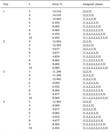
(6) Informatics in Medicine Unlocked 16 (2019) 100206. N.A. Melo Riveros, et al.. Table 3 Results of the best solutions for architecture in each test for the K-means algorithm. Test. L. Error %. Assigned classes. 1. 3 4 5 6 7 8 9 10 3 4 5 6 7 8 9 10 3 4 5 6 7 8 9 10 3 4 5 6 7 8 9 10. 14.516 14.516 12.903 6.454 8.065 8.065 6.452 6.452 12.903 12.903 9.677 9.677 4.839 8.065 8.065 8.065 11.290 11.290 12.903 8.065 6.452 8.065 9.677 8.065 12.903 8.065 9.677 8.065 6.452 9.677 8.065 6.452. [2,2,3] [2,2,3,3] [1,2,2,3,3] [1,2,2,3,3,3] [1,2,2,2,2,3,3] [1,2,2,2,2,2,3,3] [1,2,2,2,2,2,2,3,3] [1,1,2,2,2,2,2,3,3,3] [2,2,3] [2,2,2,3] [2,2,2,3,3] [1,2,2,2,3,3] [1,2,2,2,3,3,3] [1,1,2,2,2,3,3,3] [1,2,2,2,2,2,2,3,3] [1,2,2,2,2,2,2,2,3,3] [2,2,3] [2,2,2,3] [1,2,2,3,3] [1,2,2,2,3,3] [1,2,2,2,2,3,3] [1,2,2,2,2,3,3,3] [1,2,2,2,2,2,3,3,3] [1,1,2,2,2,2,2,3,3,3] [2,2,3] [2,2,3,3] [2,2,2,3,3] [1,2,2,2,3,3] [1,2,2,2,2,3,3] [1,2,2,2,2,2,3,3] [1,2,2,2,2,2,3,3,3] [1,1,2,2,2,2,3,3,3,3]. 2. 3. 4. Fig. 4. Flowchart of the SOM algorithm experimentation process.. 5. Discussion From the total solution set achieved with both of the clustering techniques (64 solutions), all of them have an error rate below 15% and 44 of them have an error lower than 10%. From Table 3, it can be deduced that the best solutions for the Kmeans algorithm were achieved with the 7 clusters architecture, which has an average classification error of 6.452% in the 4 tests. The secondbest solutions correspond to the architecture with 10 clusters, which has an average error of 7.2585%. From Table 4 it is concluded that the best solutions with the SOM algorithm were achieved with an 8-neuron grid, which resulted in an average error of 6.542%; followed by the 10neuron grid with an average error of 7.2582%. However, the third lowest average error (7.6615%) was attained by the 7-neuron architecture, which also exhibits the least generalization error of the total solution set. For K-means and SOM, the error behavior is random (Figs. 6 and 8) because of the random reorganization made to the database in each experiment. Error fluctuated widely, and it reached peaks of over 40%. However, this randomness introduced in each experiment brings a major possibility to find the global minimum of the problem without getting caught in a local minimum. Although the error rate depends on the training data, and there is a possibility of a training error being 0%, the important aspect in an artificial intelligence model is its. Fig. 5. Generalization error in relation to the clusters number for test number 2 in the K-means algorithm.. responsiveness versus new and unknown information. Thus, what matters most is its ability to generalize; hence, a model is a good solution if it responds in a satisfactory way to new data while still being as simple as possible. Regarding Figs. 5 and 7, a similar behavior is observed because the error starts from a value of 13% approximately, and then decreases until it achieves the minimum in a specific number of clusters/neurons; after this point it increases again. This behavior shows that the system exhibited a learning tendency until the minimum point was achieved; 6.

(7) Informatics in Medicine Unlocked 16 (2019) 100206. N.A. Melo Riveros, et al.. Fig. 6. Generalization error of the 1000 experiments executed for the 7 clusters during the 2nd test.. Fig. 7. Generalization error in function of the number of neurons for Test 1 in the SOM algorithm.. Table 4 Results of the best solutions for each architecture in the four tests of the SOM algorithm. Test. Grid. Error %. Assigned Classes. 1. [13] [22] [15] [23] [17] [24] [3 3] [25] [13] [22] [15] [23] [17] [24] [3 3] [25] [13] [22] [15] [23] [17] [24] [3 3] [25] [13] [22] [15] [23] [17] [24] [3 3] [25]. 12.903 12.903 11.290 4.839 8.065 6.452 8.065 6.452 14.516 12.903 8.065 9.677 4.839 6.452 8.065 4.839 14.516 11.290 11.290 11.290 8.065 6.452 8.065 9.677 12.903 9.677 12.903 9.677 9.677 6.452 8.065 8.065. [2,2,3] [2,2,3,3] [2,2,2,3,3] [1,2,2,2,3,3] [1,2,2,2,2,3,3] [1,2,2,2,2,2,3,3] [1,2,2,2,2,2,2,3,3] [1,2,2,2,2,2,2,3,3,3] [2,2,3] [2,2,3,3] [2,2,2,3,3] [2,2,2,2,3,3] [1,2,2,2,2,3,3] [1,2,2,2,2,2,3,3] [1,2,2,2,2,2,2,3,3] [1,2,2,2,2,2,2,2,3,3] [2,2,3] [2,2,2,3] [2,2,2,3,3] [2,2,2,2,3,3] [1,2,2,2,2,3,3] [1,2,2,2,2,2,3,3] [1,2,2,2,2,2,3,3,3] [1,2,2,2,2,2,3,3,3,3] [2,2,3] [2,2,2,3] [2,2,2,3,3] [2,2,2,2,3,3] [1,2,2,2,2,3,3] [1,2,2,2,2,2,3,3] [1,2,2,2,2,2,2,3,3] [1,2,2,2,2,2,2,3,3,3]. 2. 3. 4. Fig. 8. Generalization error during the 1000 experiments for the 2 × 3 grid.. SOM exhibits a higher sensibility and VPN for classes 1 and 2 while the solution with the K-means algorithm exhibits higher specificity and precision for classes 1 and 2. On the other hand, K-means exhibits higher sensitivity and VPN for class 3 while SOM exhibits higher specificity and precision for class 3. Thus the model with SOM has a greater probability of correctly classifying the patients with vertebral column problems (herniated disk or spondylolisthesis), whereas K-means has a greater probability of correctly classifying the patients without problems. From Table 9 it can be deduced that, on average, the solution with SOM presents greater sensitivity, specificity, precision and VPN regarding the solution achieved with the K-Means algorithm. From Table 10 and using the scale for the Kappa index of Table 1, it is found that for both solutions, the concordance degree is substantial. However, the solution reached with SOM has a greater concordance degree with respect to the solution achieved with the K-Means algorithm. Calculating the accuracy value of both models from the confusion 3 matrices (such as ∑i = 1 nii / N ), for K-means it is approximately 82.26% while for SOM it is 83.23%. Therefore, the model found with SOM presents a greater accuracy as a classifier as compared with the model. after this it started over-learning, increasing the generalization error. Also, it can be noticed that when assigning classes, there is a higher number of clusters associated with class 2, followed by the number of clusters associated with class 3 and finally, the number of clusters for class 1. The latter is seen in Figs. 8–10, which represent the quantity of neurons triggered by the dataset of each class in the architecture 2 × 3 of the SOM algorithm. When the data was increased, the quantity of clusters required to group increased also. This explains the class distribution pattern in the SOM neurons (Fig. 11) and the data related to the Assigned classes in Tables 3 and 4 Regarding the data in Table 8, it is deduced that the solution with 7.

(8) Informatics in Medicine Unlocked 16 (2019) 100206. N.A. Melo Riveros, et al.. Fig. 9. Neurons activated for class 1 (Herniated Disk) in the grid 2 × 3 with the SOM algorithm.. Fig. 11. Neurons activated for class 3 (Normal) in the grid 2 × 3 with the SOM algorithm.. linear kernel and another with KMOD (kernel with moderate decreasing). The accuracy values of each of these models are displayed in Table 11. The second article [30] presents 3 models. A first model that uses a multilayer neuronal network (MLP); with 6 neurons in the input layer, a hidden layer with 12 neurons, and 3 neurons in the output layer. The second uses a SVM with KMOD kernel function. And the third uses a GRNN (Generalized Regression Neural Network) with 6 neurons in the input layer, 1 hidden layer with Q radial basis functions of Gaussian type, and 3 neurons in the output layer. The accuracy values of each of these models (obtained from the confusion matrices of the best solutions for each model) are shown in Table 11. From Table 11 it is found that the model with greater accuracy is the MLP, followed by the SVMs, then by the models found with SOM and Kmeans, and finally the GRNN. It is not surprising that the MLP presents such an accuracy degree, since it is a complex model with 21 neurons. On the other hand, the SVMs are considered optimal in classification problems because they train only with the points around the separation boundary of the classes (support vectors); thus, they have a high generalization degree and avoid overfitting. However, the models of this article present a performance similar to the SVMs of the previous studies and are a simple alternative as compared to the ANNs (Artificial Neural Networks), where a greater complexity involves a greater risk of overfitting and the memorization of all in/out patterns. Moreover, our models provide an accuracy greater than 82%, and in Ref. [30] it is mentioned that this is a higher percentage than the values considered satisfactory by the orthopedic doctors who were consulted. This work presented a simple solution to classify problems of the spinal column; the database used to train the algorithms contains measurements of the spinal column that are obtained by a simple medical exam. In addition, the best models from SOM and K-means algorithms used just 6/7 neurons, less than half the neurons used in other studies, and present an accuracy acceptable for classification of patients. The models obtained (especially, the model obtained with the SOM algorithm that presents a better accuracy), can be employed in the classification of patients with spinal column problems. This model is. Fig. 10. Neurons activated for class 2 (Spondylolisthesis) in the grid 2 × 3 with the SOM algorithm.. found with K-means. Although the achieved models show a good performance, and it was found that the model got with SOM presents a better behavior compared to the model obtained with K-means, it is pertinent to compare our results with those of previous investigations concerning the diagnosis of spinal problems. For this, the results of two articles that use the same database and propose the use of other machine learning techniques in solving the problem were examined. The first article [29] proposes the use of support vector machines (SVM) and presents two models to solve the problem: an SVM with a 8.

(9) Informatics in Medicine Unlocked 16 (2019) 100206. N.A. Melo Riveros, et al.. Fig. 12. Assignation of classes for each one of the neurons for the SOM 2 × 3 grid. Table 5 Confusion matrix for architecture of 7 clusters in K-means.. C1 C2 C3 pj. C1. C2. C3. ai. 40 1 18 59. 0 135 2 137. 20 14 80 114. 60 150 100 310. Table 7 True and false positive/negative rates for each class for the best solution of Kmeans and SOM.. TP (C1) TP (C2) TP (C3) FN (C1) FN (C2) FN (C3) FP (C1) FP (C2) FP (C3) TN (C1) TN (C2) TN (C3). Table 6 Confusion matrix for architecture of 6 neurons in SOM.. C1 C2 C3 pj. C1. C2. C3. ai. 42 0 25 67. 0 145 4 149. 18 5 71 94. 60 150 100 310. K-Means. SOM. 0.6667 0.9000 0.8000 0.3333 0.1000 0.2000 0.0760 0.0125 0.1619 0.9240 0.9875 0.8381. 0.7000 0.9667 0.7100 0.3000 0.0333 0.2900 0.1000 0.0250 0.1095 0.9000 0.9750 0.8905. was assigned to class 1 (herniated disk) present a lower generalization error, considering that most of the clusters were assigned to classes 2 and 3; this is because the number of clusters is proportional, based on the quantity of data that exists for each class (see Tables 3 and 4). The randomness introduced when the database is reorganized in each experiment gives an option to determine solutions that perhaps do not represent the global minimum, but provide an acceptable generalization error given the low complexity of the models obtained (7 and 6 clusters/neurons for K-Means and SOM, respectively). Without this reorganization it could be noted that in all the experiments the same error percentage was obtained. This was noted before the experimentation see Figs. 6 and 8.. readily adaptable to any computer, and does not need specific information about the patients. If the model is employed, the classification of patients will be faster.. 6. Conclusions Firstly, from the total set of solutions reached, all of them present an error lower than 15%. About 68% of the solutions set have an error of 10% or less, requiring an average of 6 clusters/neurons. This is depicted in Tables 3 and 4 Additionally, those solutions where a cluster/neuron 9.

(10) Informatics in Medicine Unlocked 16 (2019) 100206. N.A. Melo Riveros, et al.. is the best alternative in the detection of patients with spinal problems. On the other hand, with this solution a concordance index is achieved that is substantial and is considered acceptable (since it is nearly a perfect concordance). Even when the K-means solution also achieved this concordance degree, the magnitude of the Kappa index in the SOM solution is higher (see Table 10). Finally, the solution obtained with the SOM algorithm presents a lower level of complexity than the solution obtained with the K-means algorithm, because the number of clusters is smaller, and it is considered that the simpler models are those with a greater generalization degree. The models obtained with both SOM and K-means show a satisfactory performance in comparison with other automatic learning techniques used in the diagnosis of spinal problems, such as MLP and SVMs discussed in articles [29,30]. In addition, they present a precision that, as mentioned in Ref. [29], is superior to that considered satisfactory by orthopedic doctors consulted.. Table 8 Sensibility, specificity, precision and NPV measurements for each class for the best solution of K-means and SOM.. Sensibility(C1) Sensibility(C2) Sensibility(C3) Specificity(C1) Specificity(C2) Specificity(C3) Precision(C1) Precision(C2) Precision(C3) NPV(C2) NPV(C3). K-Means. SOM. 0.6667 0.9000 0.8000 0.9240 0.9875 0.8381 0.8977 0.9863 0.7349 0.9080 0.8073. 0.7000 0.9667 0.7100 0.9000 0.9750 0.8905 0.8750 0.9748 0.7500 0.9670 0.7543. Sources of funding. Table 9 Average measurement of sensitivity, specificity, precision and NPV for the best solution of K-means and SOM.. Sensibility Specificity Precision NPV. K-Means. SOM. 0.7889 0.9165 0.9052 0.8168. 0.7922 0.9218 0.9054 0.8238. The sponsors do not have any role in the manuscript. Author contribution Nicolas Melo: Study design, data analysis, writing. Bayron Cardenas: Study design, data analysis, writing. Lilia Edith Aparacio Pico: Writing. Conflicts of interest statement. Table 10 Kappa Index for each solution obtained with K-Means and SOM algorithms.. K. K-Means. SOM. 0.7187. 0.7328. None declared. Consent The manuscript did not need studies in volunteers or patients. Acknowledgments. Table 11 Values of the accuracy of the classification models proposed in this article and in previous articles related to the diagnosis of spinal problems. Article. Model. Accuracy (%). This article. K-means SOM SVM(linear kernel) SVM(KMOD kernel) MLP SVM(KMOD kernel) GRNN. 82.26 83.23 85.00 85.90 90.32 85.48 75.80. Article [29] Article [30]. We would like to express our deep gratitude to D. Sc. Lilia E. Aparicio (our research supervisor) for her patience, guidance, encouragement and useful criticism of this research work. In addition, we want to thank our alma mater, the “Universidad Distrital Francisco José de Caldas”, for initiating us on the path of research and supporting this work. References [1] Alpaydin E. Introduction to machine learning second edition. Introduction to machine learning. 2010 Available on: https://doi.org/10.1007/978-1-62703-748-8_7. [2] González F. 2 Machine learning models in rheumatology 2. 2016. p. 77–8 Available on: http://www.scielo.org.co/pdf/rcre/v22n2/v22n2a01.pdf. [3] Rodríguez León C, García Lorenzo MM. Adecuación a metodología de minería de datos para aplicar a problemas no supervisados tipo atributo-valor [online], 8 (4). Universidad y Sociedad; 2016. p. 43–53 Available on: http://scielo.sld.cu/pdf/rus/ v8n4/rus05416.pdf. [4] Tan P-N, Steinbach M, Kumar V. Introduction to data mining. 2006. p. 496–514 Available on: https://doi.org/10.1152/ajpgi.1999.276.5.G1279. [5] Hayashi Y. Classification, diagnosis, and treatment of low back pain. Jmaj 2004;45(5):227–33. Retrieved from http://www.med.or.jp/english/pdf/2004_05/ 227_233.pdf. [6] Yee A, Mohammed S, Malcolm B, Tile M. Low back pain. The workplace safety and insurance appeals tribunal. 2016. February 2015. [7] Deyo RA, Mirza SK. Herniated lumbar intervertebral disk. N Engl J Med 2016;374(18):1763–72 Available on: http://doi.org/10.1056/NEJMcp1512658. [8] Neyra HT, Miguel IJ, Quesada D, Horacio II, Sáez T, Tabares L, Ii S. Hernia discal lumbar, una visión terapéutica Lumbar. Rev Cubana Ortop Traumatol 2016;30(1):27–39 Available on: http://scielo.sld.cu/pdf/ort/v30n1/ort03116.pdf. [9] Roman MG. Spondylolysis and spondylolisthesis. Orthopedic physical therapy secrets. third ed. 2016. p. 463–9 Available on: https://www.mayfieldclinic.com/PDF/ PE-spond.pdf. [10] Hu SS, Tribus CB, Diab M, Ghanayem AJ. Spondylolisthesis and spondylolysis. J Bone Jt. Surg 2008;90:656–71 Available on: https://pdfs.semanticscholar.org/ f93a/930aaed0b5a7738afa67754d7ef1f6b4b1d3.pdf. [11] Gonzalez Cuellar F, Obregón Neira N. Mapas auto-organizados de Kohonen como. It can be found that the better solutions to this problem were achieved with 7 clusters for K-means and 6 neurons for SOM, because after that point the generalization error increased due to the obtained model exhibiting over-learning. Although it is normal to think that models with a greater number of clusters present a lower generalization error, this also implies that the model can memorize all of the training data and not respond properly to new data (see Figs. 5 and 7). The requirements of a classifier can vary; sometimes, it is desired for it to detect patients with diseases and other times to detect patients without anomalies. Therefore, it can be concluded that the solution achieved with SOM is better at classifying correctly the cases of patients with herniated disk and spondylolisthesis, while the solution of K-means is better at detecting normal patients. Consequently, if the principal requirement is to detect patients with diseases in the vertebral column and to classify them correctly, the best solution is the SOM model - see Table 8. The solution obtained with SOM provides better results with respect to the solution obtained with K-means, because the measurements in sensibility, specificity, precision, and NPV (Table 9) are higher, and this 10.

(11) Informatics in Medicine Unlocked 16 (2019) 100206. N.A. Melo Riveros, et al.. [12] [13]. [14]. [15]. [16]. [17]. [18]. [19]. [20]. [21] Hossin M, Sulaiman M. A review on evaluation metrics for data classification evaluations. Int. J. Data Min. Knowl. Manag. Process (IJDKP) 2015;5(2):1–11 Available on: http://doi.org/10.5121/ijdkp.2015.5201. [22] Cohen J. A coefficient of agreement for nominal scales. Educ Psychol Meas 1960;20:37–46 Available on https://doi.org/10.1177/F001316446002000104. [23] Abraira V. Índice de Kappa. Semergen 2000;27:247–9 Available on: http://doi.org/ 10.1016/S1138-3593(01)73955-X. [24] Landis JR, Koch GG. The measurement of observer agreement for categorical data. Biometrics 1977;33:159–74 Available on: http://doi.org/10.2307/F2529310. [25] UCI Machine Learning Repository, Vertebral column data set. Available on: http:// archive.ics.uci.edu/ml/datasets/Vertebral+Column#. [26] Ramírez Gutiérrez R, Ramírez Minor J, Sánchez Lugo M, Juárez León B. El balance sagital en la columna lumbar degenerativa Number 3 Medigraphic 2015;11:126–33 Available on: http://www.medigraphic.com/pdfs/orthotips/ot-2015/ot153d.pdf. [27] Hay O, Dar G, Abbas J, Stein D, May H, Masharawi Y, et al. The lumbar lordosis in males and females, revisited. PLoS One 2015;10(8):e0133685https://doi.org/10. 1371/journal.pone.0133685 Available on: https://journals.plos.org/plosone/ article/file?id=10.1371/journal.pone.0133685&type=printable. [28] Koller Heiko, Acosta Frank, Hempfing Axel, Rohrmüller David, Tauber Mark, Lederer Stefan, Resch Herbert, Zenner Juliane, Klampfer Helmut, Schwaiger R, Bogner Robert, Hitzl Wolfgang. Long-term investigation of nonsurgical treatment for thoracolumbar and lumbar burst fractures: An outcome analysis in sight of spinopelvic balance. European spine journal: official publication of the European Spine Society, the European Spinal Deformity Society, and the European Section of the Cervical Spine Research Society 2008;17:1073–95. https://doi.org/10.1007/ s00586-008-0700-3. [29] Rocha Neto AR, Sousa R, Barreto GA, Cardoso JS. Diagnostic of pathology on the vertebral column with embedded reject option. Proceedings of the 5th Iberian Conference on pattern recognition and image analysis (IbPRIA'2011), Gran Canaria, Spain, 6669. 2011. p. 588–95. Lecture Notes on Computer Science. [30] Rocha Neto AR, Barreto GA. On the application of ensembles of classifiers to the diagnosis of pathologies of the vertebral column: a comparative analysis. IEEE Latin Am. Trans. 2009;7(4):487–96.. herramienta en la clasificación de ríos dentro de la metodología para la determinación de caudales ecológicos regionales ELOHA. Ing Univ 2013;17(2):311–23 Available on: https://revistas.javeriana.edu.co/index.php/iyu/ article/view/1885. Kohonen T. Essentials of the self-organizing map. Neural Netw 2013;37:52–65 Available on: http://doi.org/10.1016/j.neunet.2012.09.018. Legrand S, Elliman D. Artificial learning approaches for the next generation web: Part II, 2008, 161–169. 2008 Available on: http://www.scielo.org.mx/pdf/iit/ v9n2/v9n2a6.pdf. Miljkovic D. Brief review of self-organizing maps. 2017 40th international convention on information and communication technology. Electronics and Microelectronics (MIPRO); 2017. p. 1061–6 Available on: https://doi.org/10. 23919/MIPRO.2017.7973581. Chawan PPM, Bhonde SR, Patil S. 2 Improvement of K-means clustering algorithm Prof P M Chawan 2. 2012. p. 1378–82 Available on: http://citeseerx.ist.psu.edu/ viewdoc/download?. 10.1.1.417.1650&rep=rep1&type=pdf. Oyelade OJ, Oladipupo OO, Obagbuwa IC. Application of k-means clustering algorithm for prediction of students' academic performance. Int J Comput Sci Inf Secur 2010;7 Número 1, 292–295. Available on: https://arxiv.org/ftp/arxiv/ papers/1002/1002.2425.pdf. Tanguilig III BT, Gerardo BD, Fabregas AC. Modified selection of initial centroids for K- means algorithm. Matter: Int J Sci Technol 2016;2(2):48–64 Available on: http://doi.org/10.20319/mijst.2016.22.4864. Expósito C, Airam I, Márquez E, López I, Belén P, Batista M, Vega M. Evaluación de clasificadores n.d.Available on: https://campusvirtual.ull.es/ocw/pluginfile.php/ 15312/mod_resource/content/8/evaluacion-de-clasificadores.pdf. Freitas CO, Carvalho J M d, Oliveira Jr. JJ, Aires SBK, Sabourin R. Confusion matrix disagreement for multiple classifiers. 12th Iberoamerican congress on pattern recognition, CIARP 2007, LNCS 4756, 387–396. 2007 Available on: http://link. springer.com/chapter/10.1007/978-3-540-76725-1_41. Sokolova M, Lapalme G. A systematic analysis of performance measures for classification tasks. Inf Process Manag 2009;45(4):427–37 Available on: http://doi.org/ 10.1016/j.ipm.2009.03.002.. 11.

(12)