Collective computing

Collective Computing

González J.A.1, Leon C.1, Piccoli F.2, Printista M.2, Roda J.L.1, Rodriguez C.1 and Sande F.1

1

Universidad de La Laguna

Departamento de Estadística, I. O. y Computación

Facultad de Matemáticas. c/ Astrofísico Francisco Sánchez, s/n

38271 La Laguna S/C de Tenerife

SPAIN

2

Departamento de Informática Grupo de Interés en Sistemas de Computación

Ejército de los Andes 950 Universidad Nacional de San Luis

San Luis

{mprinti,mpiccoli}@unsl.edu.ar ARGENTINE

Abstract

The parallel computing model used in this paper, the Collective Computing Model

(CCM), is a variant of the well-known Bulk Synchronous Parallel (BSP) model.

The synchronicity imposed by the BSP model restricts the set of available

algorithms and prevents the overlapping of computation and communication.

Other models, like the LogP model, allow asynchronous computing and

overlapping but depend on the use of specific libraries. The CCM describes a

system exploited through a standard software platform providing facilities for

group creation, collective operations and remote memory operations. Based in the

BSP model, two kinds of supersteps are considered: division supersteps and

normal supersteps. To illustrate these concepts, the Fast Fourier Transform

Algorithm is used. Computational results prove the accuracy of the model in four

different parallel computers: a Parsytec Power PC, a Cray T3E, a Silicon

Graphics Origin 2000 and a Digital Alpha Server.

1.

Introduction

A computational model defines the behaviour of a theoretic machine. The goal of a model is to ease the design and analysis of algorithms to be executed in a wide range of architectures with the performance predicted by the model. The definition of a computational model limits the set of methodologies to design algorithms and how to analyse and evaluate their execution times. These methodologies restrict the design of the programming languages and guide the building of compilers that produce code for the architectures that match the model. In [Valiant 90], Valiant diagnosed the crisis of parallel computing: the main cause of the crisis is the absence of a parallel computing model that plays the role of bridge between the software and the architecture that is provided by the von Neumann model in the case of sequential computing. The conclusion of Valiant’s work is the need of a simple and precise parallel computing model that guides the design and analysis of parallel algorithms. In that work [Valiant 90], Valiant proposed the Bulk Synchronous Parallel (BSP) model. The result of the impact caused by the paper in the theoretic computation community has been the development of BSP algorithms and the software to support their implementation. This software has been specially promoted by the group of McColl and Hill in Oxford, giving place in 1996 to the Oxford BSP Library [Hill 97]. The synchronicity proposed by the BSP restricts the set of available algorithms. In 1993 Karp and Culler proposed the LogP model [Culler 93]. Culler’s group developed Active Messages [Eicken 92], a library that supports the LogP model. Afterwards, more libraries and languages oriented to this model have appeared like Fast Messages [Pakin 95] or Split C [Eicken 92].

The parallel programming standards have evolved independently of the rising of these two models. In 1989 the first version of Parallel Virtual Machine (PVM) [Geist 94] appeared. The capacity of PVM to exploit supercomputers and clusters of workstations contributed to its fast spread. In 1993 PVM was the standard “de facto”. The success of PVM leads to the first formal definition of Message Passing Interface (MPI) [Snir 96] that was presented in the ICS conference in 1994. In the following years, MPI has replaced PVM until reaching its actual position of parallel programming standard. It is necessary to emphasize that MPI offers a programming model but not a computational model. The prediction of execution times of parallel algorithms developed in MPI or PVM under BSP or LogP presents limitations and difficulties [Kort 98], [Rodriguez 98b].

Due to the difficulty for finding a computational model for current parallel architectures, the best solution until now has been to find models that predict accurately the behaviour of a restricted set of communication functions as in [Abandah 96] and [Arruabarrena 96]. In this paper we try to give a formal generalisation of this approach, the Collective Computing Model (CCM). To show how it works, we use a parallel version of the Fast Fourier Transform algorithm. The experiments were performed in a Parsytec Power PC, a Cray T3E, a Silicon Graphics Origin 2000 and a Digital Alpha Server 8400. MPI was the software platform considered.

The rest of the paper is organised as follows. The next section introduces the Collective Computing Model. Sections 3 and 4 present a comparison between the computational analysis and the experimental results obtained for the example used. In these sections we make a detailed analysis of this algorithm according to the CCM. Finally, section 5 presents some conclusions.

2.

The Collective Computing Model.

The proposed parallel computational model considers a computer made up by a set of P

the current group. The computation in the Collective Computing Model (CCM) occurs in steps that we will refer to, following the BSP terminology, as supersteps. In the model we consider two kinds of supersteps.

The first kind, called normal superstep, has two stages:

1. Local computation.

1.2.Execution of a collective communication function f from F.

The second kind of superstep defined in the CCM is the division superstep. At any instant, the machine can be divided in a certain set r of submachines with sizes P0, …,Pr-1 as a

consequence of the call to a collective partition function g∈ P. We suppose that after the division phase, the processors in the kth group are renamed from 0 to Pk

1. Distribution of the P processors in r groups of sizes P

-1. In its most general form, the division process g implies five stages:

0, …,Pr-1

1.2.Distribution of the input data, IN

(Processor Assignment)

0, …,INr-1 of the tasks to be executed (Input Data Assignment) among the P processors: in0, …,in

1.3.Execution Task

p-1 0, ..,Taskr-1

1.4.A phase of reunification (Rejoinment), and

over these input data (Task Execution)

1.5.Distribution of the results OUT0,…, OUTr-1, generated by the execution of the tasks (Result Data Assignment) among the P processors out0,…, outp-1

Some of these stages can be dropped in some division functions (for example in MPI,

MPI_Comm_Split has not associated an input data assignment, neither does it have a result data assignment stage, and the tasks in this case are only one). Therefore, a division process g is characterised by the way it does each of the five previous stages.

,.

The CCM distinguishes the communication and division costs. Associated with each collective communication function f ∈ F there is a cost function, Tf that predicts the time

invested by the communication pattern f depending on the number of processors P of the actual submachine and the length of the messages involved. Similarly, the model assumes the presence of a cost function Tg

The cost Φ

for each division pattern g ∈P.

s

Φ

of a normal superstep s, composed by a computation W, and the execution of a collective function f, is given by:

s = W + Tf = max {Wi / i = 0,…,P-1} + Tf (P, h0, …,hP-1

Where W

)

i is the time invested in computation by processor i in this superstep and hj

Let’s consider the other case, where the superstep is a division one with partition function g ∈

P. The time or cost Φ

is the amount of data (given by the maximum or the sum of the packets sent and received) communicated by processor j = 0, ..., P-1 under the pattern f and P denotes the number of processors of the current machine.

s

Φ

is given by:

s = Tg(P,in0 ,..,inP-1, r, out0 ,…, outP-1) + max{ Φ( Task0),...,Φ( Taskr-1 T

) }

g corresponds to the time invested in the division process, input data distribution,

reunification and output data interchange. The second term is the maximum of the times, recursively computed for each of the tasks Task0, ..,Taskr-1

In conclusion, the CCM is characterised bythe tuple:

associated with the call to the division function g.

(P, F, TF,P, TP

where

)

•P is the number of processors.

•F is the set of collective functions (for example, those from MPI, PVM or La Laguna C)

•TF

•P is the set of partition functions (for example the ones in MPI or La Laguna C) is the set of cost functions for each collective function in F.

Con format o: Numeración y viñetas

Con format o

•TP

Different proposals can be used to determine T

is the set of cost functions for each partition function in P.

F . For example, it would be valid to take as

TF the empirical set of linear by pieces functions obtained from Abandah’s [Abandah 96] or

Arruabarrena’s[Arruabarrena 96] studies, where latency and bandwidth are considered depending on the communication pattern. The CCM assumes a linear by pieces behaviour in the message size of the functions in TP. However, this behaviour can be non-linear in the number P

of processors (i.e. broadcast usually have a logarithmic factor in P). A similar approach could be used for obtaining TP. The dependence of the architecture allowed in the cost functions is in the

coefficients defining each particular function. Thus, once the analysis for a given architecture has been completed, the predictions for a new architecture can be obtained replacing in the formulas the function coefficients.

III.3. An Example: The Fast Fourier Transform

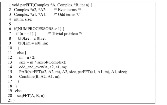
Since the use of collective functions - and their associated normal supersteps, is a common practice among MPI programmers, we will concentrate in the use of division supersteps. The code in Figure 1 showsa natural parallelization of the Fast Fourier Transform (FFT) algorithm using La Laguna C [Rodriguez 98a], a set of macros and functions that extend MPI and PVM with the capacity for nested parallelism. The algorithm takes as input a vector of complex A, and the number n of elements in that vector; and returns in vector B the transformed signal. The algorithm is based in the fact that the computation of the transform of the even and odd terms is independent and therefore can be performed in parallel.

In La Laguna C, variable NUMPROCESSORS holds the number of processors available at any instant. The algorithm begins testing if there are more than one processor in the current set. If there is only one processor, a call to the sequential algorithm seqFFT, provided by the user, occurs. Otherwise, the algorithm tests if the problem is trivial. If not, function odd_and_even()

decompose the input signal A in its odd and even components that are stored in vectors a1 and

a2 respectively. After that, the PAR construct in line 15 is employed to make two recursive calls 1 void parFFT(Complex *A, Complex *B, int n) {

2 Complex *a2, *A2; /* Even terms */ 3 Complex *a1, *A1; /* Odd terms */ 4 int m, size;

5

6 if(NUMPROCESSORS > 1) {

7 if (n == 1) { /* Trivial problem */ 8 b[0].re = a[0].re;

9 b[0].im = a[0].im; 10 }

11 else { 12 m = n / 2;

13 size = m * sizeof(Complex); 14 odd_and_even(A, a2, a1, m);

15 PAR(parFFT(a2, A2, m), A2, size, parFFT(a1, A1, m), A1, size); 16 Combine(B, A2, A1, m);

17 } 18 } 19 else

20 seqFFT(A, B, n); 21 }

Figure 1. The Fast Fourier Transform in llc.

to function parFFT in order to compute in parallel the transform of the even and odd components. The results of these computations are returned in A1 and A2respectively. The PAR

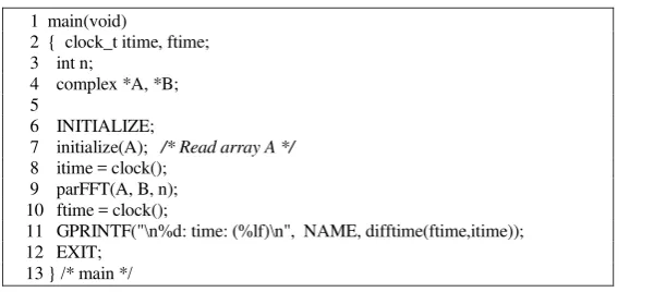
macro deals with the update of variable NUMPROCESSORS for the two sets of processors created (one dealing with the computation of the even components and the other with the odd ones) accordingly with the distribution policy implemented. Function Combine() combines the resulting transform signals A1 and A2 into the resulting vector, B. The Figure 2 shows the code corresponding to the main function.

The time invested in the division of the original vector takes time O(n), and the combination stage has the same complexity O(n).

This example is a particular case of a paradigm that we will call a common-common

algorithm. We say a problem to be solved in parallel is a common-common problem (CCP) if initially, the input data are replicated in all the processors and at the end, the solution to the problem is required to be also in all the processors. Analogously we can talk about private-private problems (PPP) as those whose input and output are distributed among the processors. Problems can be classified according to the four possible combinations: CCP, PPP, PCP, CPP. A common-common Divide and Conquer is a divide and conquer algorithm that solves a CCP. The closure property is the main advantage of the common-common computation: the composition of two common-common algorithms is also a common-common algorithm.

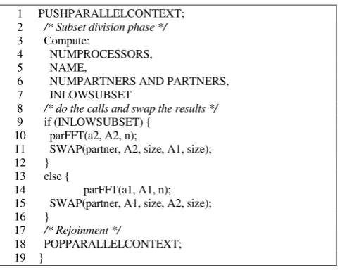
Figure 3 shows the pseudocode produced by the expansion of the PAR macro in Figure 1. In line 10, INLOWSUBSET macro divides the set of processors in two groups, G and G’. Each processor NAME in a group G chooses a processor PARTNER in the other group G’, and results are interchanged between partners.

1 main(void)

2 { clock_t itime, ftime; 3 int n;

4 complex *A, *B; 5

6 INITIALIZE;

7 initialize(A); /* Read array A */ 8 itime = clock();

9 parFFT(A, B, n); 10 ftime = clock();

11 GPRINTF("\n%d: time: (%lf)\n", NAME, difftime(ftime,itime)); 12 EXIT;

13} /* main */

Figure 2. The main() function for the code in Figure 1. Notice the same code

Figure 4 shows a set with eight processors that is divided in two groups with four processors each and the partnership relations established among the processors in the two groups when a block policy is used. The second recursive call to the PAR macro gives place to the relations presented in Figure 5. Notice that a third recursive call would give place to a set of partnership relations that form a perfect binary hypercube. Each level of parallelism corresponds to a dimension in the hypercube.

In the FFT algorithm, the groups of processors are always divided in two sets of equal size because the number of odd and even components of the signal is the same. However, it is sometimes useful to divide the set of processors in sets with different cardinals to balance the workload assigned to each processor. This is the case, for example, for any divide and conquer algorithm where the amount of work associated with each division of the problem could be different. The division of the set of processors available in subsets with different sizes can be reached in La Laguna C through the use of a different version of the PAR construct, the

WEIGHTEDPAR. If the sets have different sizes, the resulting topology is what we call a

dynamic polytope. Figure 6 shows a division process where an initial group with 6 processors 1 PUSHPARALLELCONTEXT;

2 /* Subset division phase */ 3 Compute:

4 NUMPROCESSORS, 5 NAME,

6 NUMPARTNERS AND PARTNERS, 7 INLOWSUBSET

8 /* do the calls and swap the results */ 9 if (INLOWSUBSET) {

10 parFFT(a2, A2, n);

11 SWAP(partner, A2, size, A1, size); 12 }

13 else {

14 parFFT(a1, A1, n); 15 SWAP(partner, A1, size, A2, size); 16 }

17 /* Rejoinment */

18 POPPARALLELCONTEXT; 19 }

Figure 3. Expansion of the call to the PAR macro in Figure 1.

P0 P1 P2 P3 P4 P5 P6 P7

NAME=0

NUMPROCESSORS=4 NUMPROCESSORS=4

NAME=1 NAME=2 NAME=3 NAME=0 NAME=1 NAME=2 NAME=3

Figure 4. Division phase. Each of the eight processors chose a partner in the other group.

P0 P1 P2 P3 P4 P5 P6 P7 NAME=0 NAME=1

NUMPROCESSORS= 2

NUMPROCESSORS= 2

NUMPROCESSORS= 2

NUMPROCESSORS= 2

NAME=0 NAME=1 NAME=0 NAME=1 NAME=0 NAME=1

will be divided irregularly. In the first division, the weights are w1=20 and w2=10 and therefore

four {0, 1, 2, 3} and two {4, 5} processors are assigned to each group in the first partition.

Links labelled 1 in Figure 7 show the partnership relations for this first division. If we suppose that successive divisions of the groups of processors take place like Figure 6 shows, then the left group of four processors is divided again with weights w11=11 w12=9 while the

right group is divided with weights w21=6 and w22=4. This second division “creates” a new

dimension in the dynamic polytope labelled 2 in Figure 7. The topology resulting from the division process shown in Figure 6 is the hypercube presented in Figure 7.

When there are no more processors available in the FFT code in Figure 1, the sequential algorithm seqFFT is called in line 20. The time for the sequential algorithm is

O((n/P)*log(n/P)). At the end of the recursive calls to parFFT, the partners interchange the results of their computation and a communication of n/2 Complex between partners takes place. After the interchange, both groups join in the former group.

The time Φ invested by the algorithm following the Computing Collective Model is given by the recursive expression:

Φ = D*n/2+ F*n/2 + max {Φ( parFFT(a2, A2, m)),Φ( parFFT(a1, A1, m))}+ TPAR (P,A2,...,A2,A1,...,A1)

The first term corresponds to the division process of the original signal into its components. The second term is the time corresponding to the combination of the transformed signals. D and

F are the complexity constants for the division and combination stages respectively. The third and fourth terms correspond to the division superstep. The time invested in the division

superstep is the maximum invested in each of the parallel transformations plus the time TPAR

invested in the interchange of results that takes place following the EXCHANGE pattern in a machine with P processors (first argument), without initial data distribution (the first P input parameters in0,..,inP-1 and parameter r = 2 of the model formula have been skipped) with an

interchange where each processor sends and receives m data. We can use the most convenient function TPAR.

TPAR ( P,0,...,0,2, m, ...,m) = m*gPAR+LPAR

6,5 1 0

5,4

2 3

6,4

4 5

11,9 w1= 20, w2= 10

Figure 6. Division process.

0 1

2 3

4

5

1 1

1 1

2 2

2

3 3

Figure 7. A dynamic polytope.

With a recursive reasoning, we can obtain the total time:

Φ = ∑i = 0, log(P)-1 D * n/2 i

+ C*(n/P)* log(n/P) + ∑s=1, log(P) ( gPAR* 2 s

* n/P)+LPAR+ F * 2 s-1

* n/p )

C is the complexity constant corresponding to the stage where all the processors compute the sequential FFT.

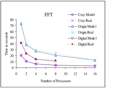
Figure 8 compares the predicted and measured times for the FFT algorithm running with a 2MB complex input vector for the Cray T3E, Silicon Graphics Origin 2000 and Digital Alpha Server. The Figure shows the accuracy of the model.

Figure 9 shows the same results for a Parsytec Power PC for a 256KB complex vector. The less accurate results are a consequence of the dependency of the network communication system.

FFT

0 10 20 30 40 50 60 70 80

0 2 4 6 8 10 12 14 16

Number of Processors

T

im

e

i

n

s

e

c

on

ds

Cray Model Cray Real Origin Mode l Origin Real Digital Mode l Digital Real

4. Conclusions

By the Collective Computing Model, we try to give a formal generalisation to find models that predict accurately the behaviour of a restricted set of communication functions. The model describes a system exploited through a library with functions for group creation and collective operations.

In the Collective Computing Model, the computation occurs in steps that we call to, following the BSP terminology, as supersteps. Two kinds of supersteps are found: normal

superstep, and the division superstep.

The Collective Computing Model suits the MPI parallel programming collective mode when running in high performance networks. The use of groups and division supersteps has been illustrated through a parallel version of the FFT in four high performance machines and the results show the model accurately when the influence of network communication is null. In other case the accuracy is less.

Acknowledgements

We wish to thank the Centre de Computació i Comunicacions de Catalunya and the Centro de Investigaciones Energéticas Medioambientales y Tecnológicas for allowing us to use their resources. Also to the Universidad Nacional de San Luis and the CONICET from which we receive continuos support.

References

[Abandah 96] Abandah, G.A., Davidson E.S. Modeling the Communication

Performance of the IBM SP2. Proc. 10th IPPS. 1996.

[Arruabarrena 96] Arruabarrena, J.M., Arruabarrena A., Beivide R., Gregorio J.A. Assesing the Performance of the New IBM-SP2 Communication Subsystem. IEEE Parallel and Distributed Technology. pp 12-22. 1996.

[Culler 93] Culler D., Karp Richard, Patterson D., Sahay A., Schauser K.E., Santos E R., von Eicken T.. LogP: Towards a Realistic Model of

Parallel Computation. Proceedings of the 4th ACM SIGPLAN, Sym. Practice of Parallel Programming. 1993.

FFT

0 1 2 3 4 5 6

0 2 4 6 8 10 12 14 16

Number of Processors

T

im

e

i

n s

e

c

onds

Parsytec Model Parsytec Real

[Eicken 92] Eicken T., Culler D.E., Goldstein S.C., Schauser K.E. Active Messages: A Mechanism for Integrated ommunication and Computation. Report No. UCB/CSD 92/#675. Computer Science Division. University of California, Berkeley, CA 94720. Mar. 1992.

[Geist 94] Geist A., Beguelin A., Dongarra J., Jiang W., Mancheck R., Sunderam V.. PVM: Parallel Virtual Machine - A Users Guide and Tutorial for Network Parallel Computing. MIT Press. 1994.

[Hambrush 96] Hambrush S.E., Khokhar A. C3

[Hill 97]

: A Parallel Model for Coarse-grained Machines. Journal of Parallel and Distributed Computing. Vol 32, nr. 2, pp. 139-154, 1996.

Hill J., McColl B., Stefanescu D., Goudreau M., Lang K., Rao B., Suel T., Tsantilas, Bisseling R.. BSPLib: The BSP Programming Library. Technical Report PRG-TR-29-97, Oxford University Computing

Laboratory. May

[Kort 98] Kort I, Trystram D. Assesing LogP Model Parameters for the IBM-SP.

EuroPar’98. LNCS Springer Verlag.

[Li 93] Li, X., Lu, P., Schaefer, J., Shillington, J., Wong, P.S., Shi, H. On the Versatility of Parallel Sorting by Regular Sampling. Parallel Computing, 19, pp. 1079-1103. 1993.

[Pakin 95] Pakin S., Lauria M., Buchanan M., Hane K., Giannini L.,Prusakova J.,

Chien A. Fast Messages on Myrinet.

[Rodriguez 98a] Rodríguez C., Sande F., Leon C. and García L. Extending Processor

Assignment Statements. 2nd

[Rodriguez 98b]

IASTED European Conference on Parallel and Distributed Systems. Acta Press. 1998.

Rodríguez C., Roda J.L., Morales D.G., Almeida F. h-relation Models for Current Standard Parallel Platforms. EuroPar’98. Springer Verlag. 1998. [Snir 96] Snir, M., Otto, S., Huss-Lederman, S., Walker, D., Dongarra, J. MPI:

The complete Reference. Cambridge, MA: MIT Press, 1996.

[Valiant 90] Valiant L.G.. A Bridging Model for Parallel Computation.