MULTIPLE CROSSOVER PER COUPLE AND FITNESS PROPORTIONAL COUPLE
SELECTION IN GENETIC ALGORITHMS
ESQUIVEL S.C., LEIVA H.A., GALLARD, R.H.
Grupo de Interés en Sistemas de Computación1 Departamento de Informática
Universidad Nacional de San Luis (UNSL) Ejército de los Andes 950 - Local 106
5700 - San Luis, Argentina.
E-mail: {esquivel, aleiva, rgallard}@inter2.unsl.edu.ar Phone: + 54 652 20823
Fax : +54 652 30224
Abstract
Contrasting with conventional approaches to crossover, Multiple Crossover Per Couple (MCPC) is an alternative, recently proposed [1], approach under which more than one crossover operation for each mating pair is allowed. In genetic algorithms, Proportional Selection (PS) is a popular method to select individuals for mating based on their fitness values.
The Fitness Proportional Couple Selection (FPCS) approach, is a new selection method which creates an intermediate population of couples from where, subsequently, couples are selected for crossing-over based on couple fitness.
This paper proposes the combined use of MCPC and FPCS. Outstanding performance was achieved by joining both methods when optimising hard testing multimodal and unimodal functions. Some of these results and their comparison against results from conventional approaches are shown.
Keywords: genetic algorithms, selection, crossover, function optimisation.
1
1. INTRODUCTION
Crossover usefulness has been extensively discussed by a number of researchers (e.g.; [3], [4], [5], [6]). The conventional approach to crossover, involves to apply the operator only once on the selected pair of parents to create, precisely, two children ([7], [8], [9], [10]). From now on we call such procedure, the Single Crossover Per Couple (SCPC) approach. In order to deeply explore the recombination possibilities of previously found solutions, in previous research we conducted several experiments in which more than one crossover operation for each mating pair was allowed.
MCPC was applied to optimize classic testing functions and harder (nonlinear, nonseparable) functions [13]. The goodness of this approach prevailed under all tests and revealed that for both sets of functions, when MCPC is applied with 2, 3 and 4 crossovers per couple, results as good as under SCPC can be expected with an additional benefit in processing time. This was obtained through the ability showed by MCPC of exploiting the recombination of good, formerly found, solutions. Those experiments, reported elsewhere [2], also showed that due to the inherent increase in selection pressure introduced by the method, a risk of premature convergence appeared reaching near optimal (suboptimal) solutions.
In order to overcome this problem we devised an strategy to combine the exploitation introduced by MCPC with the exploration of new solutions in the problem space. The latter ability was achieved by introducing a new selection operator; the Fitness Proportional Couple Selection (FPCS).
FPCS, divides the selection process into two steps; the first at individual level and the second at couple level. The method builds an intermediate population of parents which are individually selected from the old population by proportional selection, then the couples are selected according to the couple fitness. In this paper we show the results when greater fitness is associated to those couples exhibiting a greater fitness difference between their constituents. In this way, to benefit exploration, individuals likely to be distant have a greater chance to create more children than those that are residing in the neighbourhood.
The following sections describe the new selection method, the experiments performed on a set of diverse multimodal and unimodal testing functions and, finally, a comparative analysis of results is shown.
2. THE FITNESS PROPORTIONAL COUPLE SELECTION METHOD
The basic idea of FPCS is to create an intermediate population of couples, from the current population of individuals, and subsequently select for mating those pairs showing higher fitness. The criteria to assign the fitness of a couple was based on their dissimilarity. The method can be sketched as follows;
• Initially a number of individuals are selected by proportional selection to build a population of parents.
• A couple fitness value, computed as the absolute value of the difference of fitness between their components, is assigned to each mating pair.
Figure 1 shows the general FPCS scheme. As an example, suppose the following scenario; the jth couple is made by two individuals of high comparable fitness and the ith couple is formed by a medium and a low fitness individual, then there is a greater chance for the ith couple to be selected. This criterion attempts to maintain the genetic diversity to avoid stagnation but assuming a lower convergence rate.
3. TEST FUNCTIONS
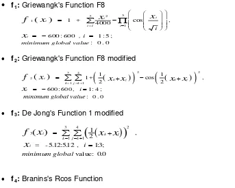
To analyse the behaviour of the new approach and following the Whitley et al. proposal [13], we selected a set compounded by nonlinear, unimodal, multimodal and nonseparalble testing functions [11], [12], [14], [15]. They were:
• f1
f x x x
x i i i i i i
minimum global value 1
2 1 5
1 4000
600 600 1 5
0 0
( ) cos ,
: : ;
: . +
, i i=1 5 = − = − = ∑ ∏ = : Griewangk's Function F8
• f2: Griewangk's Function F8 modified
(
)
(
)
(
(
)
)
f x x x x x
x
i k j k j
j k k
i i
minimum global val
2 2 2 1 4 1 3 1 1 2 1 2
600 600 1 4
0 0
( ) cos ,
: , : ; : . + = + − + = − = = + = ∑ ∑ ue
• f3: De Jong's Function 1 modified
(
)
(
)
f
x
x
x
x
i k j
j k k i i minimum global 3 2 1 4 1 3 1 2
512 512 1 3 0 0
( )
: : ; : . , = - . . , value= + = = + =
∑
∑
• f4: Branins's Rcos Function
Individual-k2 Individual -i1 Individual -j1 Individual -j2 Individual -i2 Individual -k1 Individual-1k Individual -2k Individual -1i Individual -2i Couple-i Couple -j Couple -k
1st selection 2nd selection + op.
Parents Population
Current Generation Next generation
n
n/2
n
1st Selection: proportional selection to the individual fitness.
2nd selection + op: proportional selection to the couple fitness plus classic genetic operators.
Couple fitness = |mate1.fitness - mate2.fitness|.
[image:3.595.83.426.493.768.2]n: population size.
(
)
( )f
x x
x
x
x
minimum
4 1 2
2 2
2
1 1 1
1
5 1
4
5
6 10 1 1
8 10
5 10 0 15 0 397887
(
,)
. cos( ) ,: , : ; : .
= x
x
x
= global value 2 2 − ⋅ ⋅ + ⋅ − + ⋅ − ⋅ + − =
⋅
π π π• f5: Easom's Function
( ) ( ) ( ) ( )
f x x x x x x
x
e
minimum global value i
5 1 2 1 2
2
1 2 2
100 100 1 2 1
( , ) cos cos
: , : ; : , i = − ⋅ ⋅ − − + − = − = − π π
• f6: Rastrigin's Function
( )
(
( ))
f
x
x
x
x
i i i
i n i n 6 2 1
10 10 2
5 12 5 12 5 0 0 =
= n minimum global value
⋅ + − ⋅ ⋅ ⋅
− =
=
∑
cos ,. : . , ; : .
π
4. EXPERIMENTAL TESTS
Many series, with randomised initial population, of 6 runs each one, were performed on every function, in such a way that run 1 performed only one crossover per couple (SCPC) and run i (2 ≤ i≤ 6) executed exactly i crossovers, that means 2i children, per couple (MCPC). In every case each new created offspring was inserted into the next generation, until the population size was reached. We make reference here only to four of those experiments:
Experiment Crossover Probability Mutation Probability # of generations
E1 .50 .005 2500
E2 .50 .005 3000
E3 .50 .005 4000
[image:4.595.81.476.76.327.2]E4 .50 .005 5000
Table 1: Parameters of the MCPC GA used in diverse experiments.
The experiments were based on a simple, but not canonical, Genetic Algorithm, [14], [15] with binary coded chromosomes, elitism, bit swap mutation, one point crossover and population size fixed to 70 individuals. In the case of the Easom’s function the probabilities were set to 0.65 and 0.05 for crossover and mutation respectively. Due to the increase in selective pressure introduced by MCPC it was observed that the reduction of running time was paid by being more distant from the known or estimated optimum value. Hence, the range of this error is an important issue to consider.
The following relevant performance variables were examined:
Ebest = ((opt_val - best value)/opt_val)100
It is the percentile error of the best found individual when compared with opt_val2
Epop (Ep) = ((opt_val - mean pop value)/opt_val)100
. It gives us a measure of how far are we from that opt_val.
It is the percentile error of the population mean fitness when compared with opt_val. It tell us how far the mean fitness is from that opt_val.
Gbest (Gb) : Indicates the generation where the best valued individual (retained by elitism) was found.
2
Itime (It) = ((Tm - To)/To)100, where To = T
running time using proportional selection m =
Running time increment. It is the percentile of time increase when compared with classic selection.
running time using FPCS.
All the values analysed were mean values obtained from the many series for each fixed number of crossovers completed, on each function.
5. A GENERAL OUTLOOK ON RESULTS
After accomplishing the experimental runs, the following statistical analysis were done:
I. A general overview for MCPC values contrasted with the corresponding SCPC values, under FPCS. Mean values for the first three of the above mentioned performance variables were studied. This was done for all functions and experiments.
II. A comparative analysis between the effects of the new FPCS method and
proportional selection for all of the above mentioned variables, on every function over all the experiments, contrasting results under SCPC and MCPC.
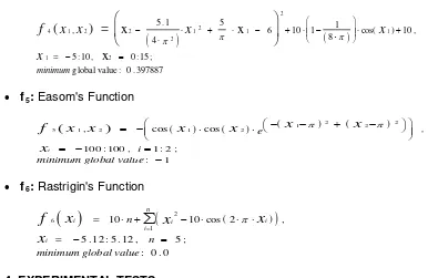
Table 2 and figure 2, show results from statistical analysis I (mean values over all experiments), corresponding to the parameters set indicated in section 4. In what follows, the discussion should be followed by looking also to the appendix on fitness landscapes.
[image:5.595.116.489.497.640.2]#cross f1 f2 f3 f4 f5 f6 1 0.06175 0.00140 0.00000 0.00216 0.64013 0.03238 2 0.06448 0.00140 0.00000 0.00216 1.26583 0.00005 3 0.05557 0.00140 0.00000 0.00216 0.01228 0.07557 4 0.05754 0.00140 0.00000 0.00216 1.26507 0.12970 5 0.07048 0.00140 0.00000 0.00216 1.26713 0.13129 6 0.06285 0.00140 0.00000 0.00216 0.01505 0.16078
Table 2. Ebest values for each test function
#CROSS 0
0.2 0.4 0.6 0.8 1 1.2 1.4
1 2 3 4 5 6
F1 F2 F3 F4 F5 F6
Fig. 2. Ebest values for each test function
Observing the above table and figure it can be concluded that better result values are achieved when a number of 2 to 4 crossovers is allowed per selected couple. Running the experiments, functionsf2, f3 and f4showed to be easy to optimise for the simple GA under FPCS while f1(highly multimodal), f5 (unimodal and highly deceptive for a simple GA) and f6 (highly multimodal) showed to be the more difficult ones to optimise.
selected couple. This result shows the effectiveness of the exploitation of previous good results when the search process was lucky and free of stagnation (some individuals fall into the hole). Consequently it is recommended to introduce some further criteria to guide the search.
Now some details on the results of the experiments over the most interesting functions (f1 and f5) is shown in the following discussion. Only some discussion on f6 , and not detailed information, is also included because similar results were obtained with f1.
5.1 MCPC VERSUS SCPC UNDER FPCS
FUNCTION F1: Typical Griewank’s function F8
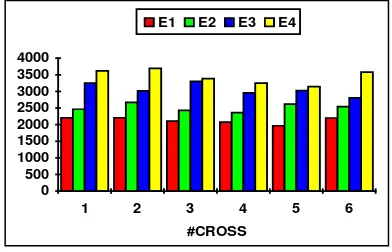
#cross E1 E2 E3 E4 1 0.077717 0.062612 0.058653 0.048016 2 0.072343 0.065930 0.066127 0.053532 3 0.065673 0.053601 0.059071 0.043947
4 0.074566 0.061527 0.049691 0.044358
[image:6.595.308.502.229.344.2]5 0.065718 0.083368 0.068639 0.064204 6 0.080176 0.061837 0.049286 0.060086
Fig. 3. Ebest values for function f1
As shown in figure 3 when the number of generations is incremented, results are improved. In many instances, for the values shown in boldface MCPC defeats SCPC. It happens, particularly, when the number of crossovers allowed is 3 or 4. The best value for Ebest was obtained for 3 crossovers and 5000 generations.
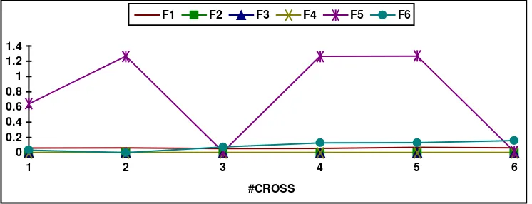
[image:6.595.307.503.446.572.2]#cross E1 E2 E3 E4 1 2202 2463 3252 3617 2 2208 2668 3018 3692 3 2108 2433 3303 3385 4 2079 2360 2958 3254 5 1967 2617 3028 3146 6 2200 2545 2805 3580
Fig. 4. Gbest values for function f1
Figure 4 indicates that when the number of generations is incremented the best individual is found at a later stage of the evolutionary process. This ensure a slower but a better convergence to the optimum as it is confirmed by the values of Ebest
shown above.
#CROSS 0
0.02 0.04 0.06 0.08 0.1
1 2 3 4 5 6
E1 E2 E3 E4
#CROSS 0
500 1000 1500 2000 2500 3000 3500 4000
1 2 3 4 5 6
#cross E1 E2 E3 E4 1 25.3028 24.5810 27.0611 26.4806 2 25.5282 26.1561 24.9862 22.9136 3 26.1285 25.0881 24.9649 26.5468 4 27.3112 26.4273 25.2620 26.7178 5 25.3753 23.3847 26.4615 25.4626 6 25.7223 27.5452 25.9428 25.7632
Fig. 5. Epop values for function f1
Running under FPCS, Epop values are relatively high for the f1 function . This was expected because we tried tentatively to reduce the selective pressure introduced by MCPC by assigning highest fitness to dissimilar couples. Consequently the difficulty of a simple GA to develop niches with a considerable number of outperformers is increased and the risk of stagnation reduced in multimodal functions. This is remarkably observed in harder functions such as f1 and f6, where results are similar.
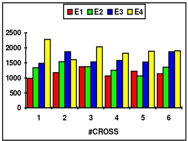
FUNCTION f5: Easom's Function
#cross E1 E2 E3 E4 1 0.018987 0.014531 2.514529 0.012455 2 0.015569 2.515568 0.018682 2.513492 3 0.012456 0.015569 0.010700 0.010379
[image:7.595.311.497.352.487.2]4 2.512528 2.517642 0.012454 0.017643 5 5.016604 0.018683 0.017644 0.015569 6 0.013493 0.017659 0.018682 0.010380
Fig. 6. Ebest values for function f5
For the f5, very hard unimodal function, it can be observed that mean values of Ebest
are in general better for 3 and 6 crossovers per couple. For these number of crossovers all the percentile error values are less than 0.02% over all experiments. It does not happens under SCPC.
[image:7.595.313.499.592.732.2]#cross E1 E2 E3 E4 1 987 1339 1487 2280 2 1176 1543 1870 1607 3 1375 1371 1532 2035 4 1066 1254 1584 1820 5 1223 1067 1529 1890 6 1140 1356 1870 1900
Fig. 7. Gbest values for function f5
#CROSS 0
1 2 3 4 5 6
1 2 3 4 5 6 E1 E2 E3 E4
#CROSS 0
500 1000 1500 2000 2500
1 2 3 4 5 6 E1 E2 E3 E4
#CROSS 0
5 10 15 20 25 30
The above table and figure show that when the number of generations is increased then the best individual is found later. This is an indication of the slower convergence rate to the optimum for this function.
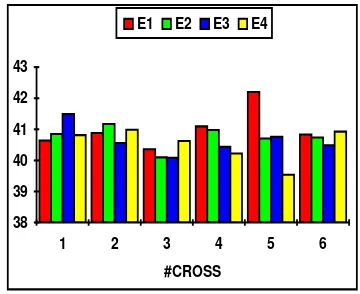
[image:8.595.317.497.115.262.2]#cross E1 E2 E3 E4 1 40.6430 40.8518 41.4920 40.8122 2 40.8842 41.1716 40.5584 40.9890 3 40.3601 40.0976 40.0865 40.6230 4 41.0940 40.9782 40.4342 40.2207 5 42.2002 40.7074 40.7598 39.5367 6 40.8346 40.7405 40.4883 40.9275
Fig. 8. Epop values for function f5
Epop values for the f5 function are the highest of the testing set when running under FPCS. This effect can be explained because there is a very low probability for individuals to find the hole where the optimum value can be met; a needle in a haystack problem. Also here the simple GA is unable to grow a niche with many outstanding individuals. Conversely many of them remains in the plate zone of the fitness landscape and this, in fact, affects the mean fitness of the population.
Now we pass to discuss some results on statistical analysis II; the comparison between FPCS and PS when applied to MCPC and SCPC.
5.2 FPCS VERSUS PS
FUNCTION f1: Typical Griewank’s function F8
#cross PS FPCS 1 0.10829 0.06175 2 0.10870 0.06448 3 0.11620 0.05557 4 0.12142 0.05754 5 0.11889 0.07048 6 0.11515 0.06285
Fig. 9. Ebest for f1
The table and figure for Ebest in f1 shows a significant reduction of the error which is about of 50% on each number of crossovers. The values shown above are outcomes from over all experiments. This important results is replicated and even improved for the Rastrigin (f6) function. Consequently these evidence supports the hypothesis that the new approach is highly recommended for optimising hard multimodal functions.
#CROSS 0
0.05 0.1 0.15
1 2 3 4 5 6 PS FPCS
#CROSS 38
39 40 41 42 43
1 2 3 4 5 6
#cross PS FPCS 1 1458 2884 2 1744 2896 3 1953 2807 4 1993 2663 5 1958 2690 6 1973 2782
Fig. 10. Gbest for f1
Throughout the experiments and for any number of crossovers under FPCS the best value is found later than under PS. This is the expected consequence of choosing dissimilar couples to avoid stagnation.
[image:9.595.344.491.281.406.2]#cross PS FPCS 1 9.544 25.856 2 9.810 24.896 3 10.457 25.682 4 9.612 26.430 5 11.347 25.171 6 11.001 26.243
Fig. 11. Epop for f1
Epop values are higher for the f1 function under FPCS than under PS. Under FPCS, to avoid the risk of stagnation, we assign highest fitness to dissimilar couples. As a consequence the population remains disseminated on the fitness landscape and few outperformers are created. This natural consequence can be notably observed in both multimodal functions, f1 and f6.
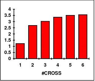
#cross FPCS 1 1.22 2 2.69 3 3.02 4 3.36 5 3.51 6 3.56
Fig. 12. Itime for f1
Increments of processing time under FPCS for f1 varies from 1 to 4 %. These values are similar for all functions.
FUNCTION f5: Easom's Function
#CROSS 0
1000 2000 3000
1 2 3 4 5 6 PS FPCS
#CROSS 0
10 20 30
1 2 3 4 5 6 PS FPCS
#CROSS 0
0.5 1 1.5 2 2.5 3 3.5 4
[image:9.595.343.498.535.667.2]#cross PS FPCS 1 0.39515 0.64013 2 0.03856 1.26583 3 0.06548 0.01228
[image:10.595.339.510.38.195.2]4 0.31116 1.26507 5 0.10053 1.26713 6 0.04772 0.01505
Fig. 13. Ebest values for function f5
For function f5Ebest values are in general better under PS than under FPCS, but the best values are recorded under FPCS with 3 and 6 number of crossovers.
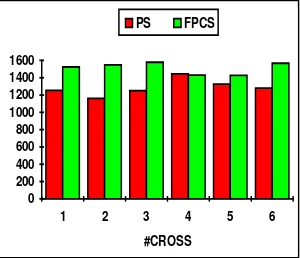
[image:10.595.347.497.286.415.2]#cross PS FPCS 1 1253 1523 2 1161 1549 3 1251 1578 4 1443 1431 5 1325 1427 6 1279 1567
Fig. 14. Gbest values for function f5
Again under FPCS the best valued individual is found later than under PS, but differences with PS are not so high as with multimodal functions.
# cross PS. FPCS 1 48.666 40.950 2 48.657 40.901 3 48.263 40.292 4 48.025 40.682 5 48.484 40.801 6 48.720 40.748
Fig. 15. Epop values for function f5
Epop values for the f5 function are the highest of the testing set under both selective approaches. For this unimodal function it is unlikely, by using a simple GA, to find the way to the basin and most of the individuals remains in the plane. Consequently it is difficult to find, initially, individuals with much different fitness and the FPCS strategy behaves not so efficiently as expected. Another ways of providing genetic diversity, such us selecting different parameters sets, must be devised.
#CROSS 0
0.5 1 1.5
1 2 3 4 5 6 PS FPCS
#CROSS 0
200 400 600 800 1000 1200 1400 1600
1 2 3 4 5 6
PS FPCS
#CROSS 0
10 20 30 40 50
[image:10.595.345.503.506.645.2]6. CONCLUSIONS
The paper discusses a hybrid approach; combining MCPC and FPCS methods for crossover and selection. The rational behind this approach relies in the attempt to diminish the selective pressure introduced by MCPC, seeking for higher quality of solutions. In this work we attempted indirectly to improve genetic diversity by assigning higher fitness to dissimilar couples expecting a consequently greater distance between parents in the fitness landscape.
The approach is quite successful for classic testing functions f2, f3 and f4 and for highly multimodal hard functions such as f1 and f6, but results are not as good when a deceptive hard unimodal function as f5 is undertook. As results are promising, and in order to find possible extensions of the hybrid approach, the investigation will be addressed to further refinements including varied parameters sets and guided convergence for unimodal hard functions.
7. ACKNOWLEDGEMENTS
We acknowledge the cooperation of the project group for providing new ideas and constructive criticisms. Also to the Universidad Nacional de San Luis and the CONICET from which we receive continuous support.
8. BIBLIOGRAPHY
[1] Esquivel S., Gallard R. and Michalewicz Z., Another Approach to Crossover in Genetic Algorithms, Proceeding of Primer Congreso Argentino de Ciencias de la Computación, pages 141 - 150, 1995.
[2] Esquivel S., Leiva C. and Gallard R., Multiple Crossover per Couple in Genetic Algorithms, Proceeding of Fourth IEEE International Conference on Evolutionary Computation, pages 103 - 106, Indianapolis, USA, 1997.
[3] Schaffer J. and Eshelman L., On Crossover as an Evolutionary Viable Strategy, in Fourth International Conference on Genetic Algorithms, pages 61 -68, 1991.
[4] Spears W.M, A Study of Crossover Operators in Genetic Programming, in International Symposium on Methodologies for Intelligent Systems, pages 409 - 418, 1991.
[5] Eshelman L. and Schaffer D., Crossover’s Niche, in Fifth International Conference on Genetic Algorithms, pages 9 - 14, 1993.
[6] Fogel D. and Stayton L., On the Effectiviness of Crossover in Simulated Evolutionary Optimization, Biological Cybernetics, Vol. 32, pages 171 - 182, 1994.
[7] Davis L., Adapting Operator Probabilities in Genetic Algorithms, in Third International Conference on Genetic Algorithms, pages 61 -69, 1989.
[8] Davis L., Job Shop Scheduling with Genetic Algorihms, in International Conference on Genetic Algorithms and their Applications, pages 136 - 140, 1985.
[9] Frantz D. R., Non Linearities in Genetic Adaptive Search, Dissertation Abstracts International, 33(11), 5240B - 5241B.
[10] Sysweda G., Uniform Crossover in Genetic Algorithms, in Third International Conference on Genetic Algorithms, pages 2 - 9, 1989.
[11] De Jong K. A., Analysis of the Behavior of a Class of Genetic Adaptive Systems, PhD Dissertation, University of Michigan, 1975.
[13] Whitley D.,Mathias K., Rana S., Dzubera J., Building Better Test Functions, Proceedings of the Sixth International Conference on Genetic Algorithms, pages 239-246, 1995.
[14] Goldberg D.E., Genetic Algorithms in Search Optimization and Machine Learning, Addison Wesley Publishing, 1989.