The impacts of non traditional exports on income, child health and education in rural Zambia

(1)

THE IMPACTS OF NON TRADITIONAL EXPORTS ON INCOME, CHILD HEALTH AND EDUCATION IN RURAL ZAMBIA

JORGE BALAT

RESUMEN

Clasificación JEL: I32, Q12, Q17, Q18

Este trabajo investiga el impacto de exportaciones no tradicionales en familias rurales en Zambia. La identificación y estimación de los efectos de largo plazo es lo que distingue a este trabajo de la literatura actual. Estudiamos los impactos en el ingreso, salud y educación infantil utilizando métodos de propensity score matching. Encontramos efectos positivos en el ingreso de las familias involucradas en actividades agrícolas de mercado por sobre las involucradas en agricultura de subsistencia. Mientras encontramos que los niños viviendo en familias productoras de algodón tienden a mostrar mejores resultados antropométricos en el largo plazo, no se observan diferencias sistemáticas en familias involucradas en otras actividades agrícolas. Finalmente, encontramos que las familias en agricultura de mercado tienden a educar más a sus hijos. Hay alguna evidencia que los niños se benefician mas que las niñas.

Palabras clave: Exportaciones agrícolas, pobreza, antropometría, educación.

ABSTRACT

JEL Classification: I32, Q12, Q17, Q18

This paper investigates the impacts of non-traditional exports on household outcomes in rural Zambia. It is the attempt to identify and estimate second round effects that distinguishes this paper from most of the current literature. We study the impacts on income, child health and education using a propensity score matching methodology. We find positive income differentials of households involved in market agriculture over subsistence agriculture. While we find that children living in households involved in cotton tend to show better long-run anthropometric outcomes, no systematic differences are observed in households engaged in other agricultural activities. Finally, we find that households in market agriculture tend to educate their children more. There is some evidence that boys are benefited more than girls.

(2)

THE IMPACTS OF NON TRADITIONAL EXPORTS ON INCOME,

CHILD HEALTH AND EDUCATION IN RURAL ZAMBIA1

JORGE BALAT2

I. Introduction

Zambia has been an exporter of copper products since Independence. When prices were high, the country was able to develop and to finance a large number of parastatal organizations and a large system of production and consumption subsidies. The decline in copper prices brought about a decline in economic growth, fiscal insolvency and poverty. During the last decade, the country adopted several economic reforms, including macroeconomic stabilization measures, trade liberalization, export promotion, and the elimination of marketing boards in maize and cotton. Some of these reforms were directed at generating incentives for the growth of non-traditional exports, like cotton, agro-processed food, tobacco, and vegetables. This growth in agricultural exports is expected to benefit households, particularly in remote rural areas.

In this paper, we study the effects of non-traditional exports on household outcomes. The majority of the literature examines the income dimension of trade. Here, we investigate the impacts on income, but also on other non-monetary outcomes. More concretely, we look at the effects on child health and education, major indicators of welfare. In terms of the health outcomes of Zambian children, we examine the impacts on different anthropometric indicators like height-for-age, weight-for-age, and weight-for-height. In terms of educational outcomes, we examine the years of formal education reported by the children.

We are interested in exploring some of the dynamic effects of international trade on rural areas and agricultural activities. By facilitating access to larger

1

This paper is based on my Master’s thesis. I am greatly indebted to Guido Porto for his invaluable support, advice and guidance through the entire process of writing this paper. Also I wish to thank M. Olarreaga and Bank-Netherlands Partnership Program (BNPP). All errors are my responsibility.

2

(3)

international markets and by boosting non-traditional export sectors, trade provides incentives for rural households to move from subsistence to market-oriented agriculture. To capture these effects, we identify relevant agricultural activities, by providing a detailed description of household productive activities, and we estimate the differences in outcomes generated by market agriculture over subsistence agriculture using matching methods. These estimates provide a quantification of the monetary and non-monetary gains that may arise due to access to international markets and to the expansion of non-traditional exports. It is this attempt to identify and estimate second round effects of increased market opportunities in rural areas that distinguishes this paper from most of the current literature.

The paper is organized as follows. In Section II, we describe the pattern of trade observed in Zambia during the 1990s, and we briefly highlight some of the main reforms in cotton and maize markets. We provide a poverty profile, too. In section III, we carry out the matching exercises. We look at sources of income and we estimate income differential gains in market agriculture. We also estimate the observed differences in child health and education. Section IV concludes.

II. Trade and Poverty in Zambia

Zambia is a landlocked country located in southern central Africa. Clockwise, neighbors are Congo, Tanzania, Malawi, Mozambique, Zimbabwe, Botswana, Namibia, and Angola. In 2000, the total population was 10.7 million inhabitants. With a per capita GDP of only 302 US dollars, Zambia is one of the poorest countries in the world and is considered a least developed country.

(4)

A. Poverty

Zambia faces two poverty ordeals: it is one of the poorest countries in the world, and it suffered from increasing poverty rates during the 1990s. The analysis of the trends in poverty rates can be done using several household surveys. There are four of them in Zambia, two Priority Surveys, collected in 1991 and 1993, and two Living Conditions Monitoring Surveys, in 1996 and 1998. All these surveys have been conducted by the Central Statistical Office (CSO) using the sampling frame from the 1990 Census of Population and Housing.

The Priority Survey of 1991 is a Social Dimension of Adjustment (SDA) survey. It was conducted between October and November. The survey is representative at the national level and covers all provinces, rural and urban areas. A total of 9,886 households were interviewed. Questions on household income, agricultural production, non-farm activities, economic activities, and expenditures were asked. Own-consumption values were imputed after the raw data were collected. Other questions referred to household assets, household characteristics (demographics), health, education, economic activities, housing amenities, access to facilities (schools, hospitals, markets), migration, remittances and anthropometry.3

The 1996 and 1998 Living Conditions Monitoring Surveys expanded the sample to around 11,750 and 16,800 households respectively. The surveys included all the questions covered in the Priority Survey of 1991, expanded the questionnaires to issues of home consumption and coping strategies, and gathered more comprehensive data on consumption and income sources.

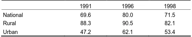
Table 1 provides some information on poverty dynamics. In 1991, the poverty rate at the national level was 69.6 percent. Poverty increased in 1996, when the head count reached 80 percent, and then declined towards 1998, with a head count of 71.5 percent. In rural areas, poverty is widespread; the head count was 88.3 percent in 1991, 90.5 percent in 1996 and 82.1 percent in 1998. Urban areas fared better, with a poverty rate of 47.2 percent in 1991, 62.1 percent in 1996 and 53.4 percent in 1998.

In Table 2, a more comprehensive description of the poverty profile, by provinces, is provided for 1998. Zambia is a geographically large country, and

3

(5)

provinces differ in the quality of land, weather, access to water, and access to infrastructure. The capital Lusaka and the Copperbelt area absorbed most of the economic activity particularly when mining and copper powered the growth of the economy. The Central and Eastern provinces are cotton production areas. The Southern Province houses the Victoria Falls and benefits from tourism. The remaining provinces are less developed.

There were significant differences in the poverty rates across regions. All provinces showed aggregate poverty counts higher than 60 percent, except for Lusaka, the capital (48.4 percent). Poverty in Copperbelt was 63.2 percent and in Southern, 68.2 percent. The highest head count was observed in the Western province, where 88.1 percent of the total population lived in poverty. The other provinces showed head counts in the range of 70 to 80 percent. Poverty was much higher in rural areas than in urban areas. Even in Lusaka, a mostly urban location, rural poverty reached over 75 percent. In the Western province, 90.3 percent of the rural population lived in poverty in 1998. Urban poverty was lower, never exceeding 70 percent of the population (including the Western province).

B. Major Reforms

The Republic of Zambia achieved Independence in 1964. A key characteristic of the country is its abundance in natural resources, particularly mineral deposits (like copper) and land. Due to high copper prices, the new Republic did quite well in the initial stages of development. Poverty and inequality, however, were widespread and this raised concerns among the people and the policymakers. Soon, the government began to adopt interventionist policies, with a much larger participation of the state in national development. Interventions included import substitution, price controls of all major agricultural products (like maize), nationalization of manufacturing, agricultural marketing and mining.

(6)

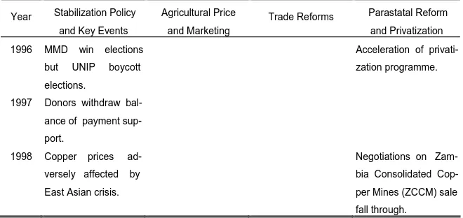
In 1991, the Movement for Multi-Party Democracy (MMD) was elected. Faced with a sustained, severe recession and with a meager future, the new government began economy-wide reforms including macroeconomic stabilization, exchange rate liberalization, fiscal restructuring, removal of maize subsidies, decontrol of agricultural prices, privatization of agricultural marketing, and trade and industrial policy. Table 3, reproduced from McCulloch et al. (2001), describes the major reforms adopted during the 1990s.

C. Maize Reforms

Fueled by high copper prices and exports, Zambia maintained, during the 1970s and 1980s, large systems of maize production and consumption subsidies. They were administered by marketing boards. External shocks (the collapse of copper prices) and inappropriate domestic policies made marketing boards unsustainable and led to their elimination in the reforms of the 1990s. The removal of the distortions were supposed to bring about aggregate welfare gains. In practice, the effects on household welfare critically depended on complementary policies like the provision of infrastructure and the introduction of competition policies.4

Maize prices affect the real incomes of poor households significantly because the poor allocate a substantial part of their budget to maize meal and because Zambian farmers can derive a large fraction of their cash income from maize crops. Poor urban households are net maize consumers; poor rural households can be either net producers or purchasers of maize. The elimination of maize subsidies and the accompanying complementary policies had significantly different impacts on the poor, depending on whether they lived in rural or urban areas, and whether they were net sellers or net buyers of maize.

Maize pricing policies affected each of producer and consumer prices. Pan-territorial maize producer prices were fixed for each harvest year, and only sanctioned government agents were allowed to participate in maize marketing. In addition to subsidies in the form of uniform producer prices regardless of location and season, direct subsidies were often provided for productive inputs and transport. Maize meal (breakfast and roller meal) was subsidized as well.

4

(7)

Since maize is the main staple and a key agricultural produce of Zambian households, the marketing board worked as a redistribution mechanism to fight poverty.

In 1993, the government began reforming the maize pricing and marketing system, eliminating subsidies, and removing international trade restrictions. The most important reforms consisted of the removal of all price controls (including pan-territorial and pan-seasonal pricing), and the decentralization of maize marketing and processing. At present, the marketing board has been fully eliminated. However, as of 2001, the government implemented a floor price for production of maize.

The removal of the marketing board implied large changes in the prices faced by maize producers and consumers. On the production side, the elimination of the pan-territorial pricing included a subsidy to transportation costs that benefited remote, usually poorer households. The elimination of these subsidies without the provision of improved transport infrastructure led to a decline in net producer prices. While the income of many Zambian households was reduced, producer markets were completely shut down for many others.

On the consumption side, the government subsidized maize to consumers by regulating maize milling and sales. Large-scale mills located in urban centers distributed industrial maize (breakfast and roller meal) throughout the country and controled most of the market for maize meal. Small-scale mills (hammermills) were not allowed to participate in maize marketing. Their function was to mill own-produced grain for home consumption. Because of the subsidies to production and industrial maize, it was often cheaper for rural consumers to sell their harvested maize and buy cheap milled maize.

(8)

There is a caveat, though. In times of production shortages, Zambia resorts to imported maize to satisfy food needs. Traditionally, industrial large-scale mills, as opposed to hammermills, have been able to import maize or have been granted preferential access to publicly imported grain (Mwiinga et al., 2002). These constraints on small-scale mills can force households to consume larger shares of industrial maize, and lower shares of mugaiwa meal, with consequent welfare costs in terms of food security.

D. Cotton Reforms

The cotton sector was significantly affected by the agricultural reforms adopted by Zambia during the 1990s.5 Before 1994, intervention in cotton markets was widespread and involved setting prices for sales of certified cotton seeds, pesticides, and sprayers, providing subsidized inputs to producers, facilitating access to credit, etc. From 1977 to 1994, the Lint Company of Zambia (Lintco) acted as a nexus between local Zambian producers and international markets. Lintco had a monopsony in seed cotton markets, and a monopoly in inputs sales and credit loans to farmers.

The reforms of the mid-1990s eliminated most of these interventions and markets were liberalized. Since Lintco was sold to Lonrho Cotton in 1994, a domestic monopsony developed early after liberalization. As market opportunities arose, several firms (private ginners such as Swarp Textiles and Clark Cotton) entered the Zambian cotton market. This initial phase of liberalization, however, did not succeed in introducing much competition in the sector. This is because the three major firms segmented the market geographically. In consequence, liberalization gave rise to geographical monopsonies rather than national oligopsonies.

At that moment, Lonrho and Clark Cotton developed an outgrower scheme with the Zambian farmers. This scheme allowed ginners to expand production and take advantage of economies of scale and idle capacity. In these outgrower programs, firms provided seeds and inputs on loans, together with extension services to improve productivity. The value of the loan was deducted from the sales of cotton seeds to the ginners at picking time. Prices paid for the harvest supposedly depended upon international prices. Initially, repayment rates were

5_{For more details on cotton reforms in Zambia, see Food Security Research Project (2000) and}

(9)

high (around roughly 86 percent) and cotton production significantly increased.

By 1997, the expansion of the cotton production base attracted new entrants, such as Amaka Holdings and Continental Textiles. Instead of the localized monopsonies, entrants and incumbents started competing in many districts. As a result of entry, the capacity for ginning increased beyond production levels. This caused an excess demand for cotton seeds and tightened the competition among ginners for Zambian cotton. In addition, some entrants that were not using outgrower schemes started offering higher prices for cotton seeds to farmers who had already signed contracts with other firms. This caused repayment problems and increased the rate of loan defaults.

The relationship between ginners and farmers started to deteriorate. On top of all this, world prices began to decline, and farm-gate prices declined as a result. After many years of high farm-gate prices, and with limited information on world market conditions, farmers started to mistrust the ginners and suspicions of exploitation arose. In consequence, farmers felt that outgrowers contracts were being breached, and default rates increased. This led firms to increase the price of the loans charged to farmers, who, in the end, received a lower net price for their crops.

Partly as a result of this failure of the outgrower scheme, Lonrho announced its sale in 1999 and Dunavant Zambia Limited entered the market. Nowadays, the major players in cotton markets in Zambia are Dunavant (Z) Limited, Clark Cotton Limited, Amaka Holdings Limited, Continental Ginneries Limited, Zambia-China Mulungushi Textiles and Mukuba Textiles.

(10)

E. Trade Trends

Zambia's major trading partners are the Common Market for Eastern and Southern Africa (COMESA), particularly Zimbabwe, Malawi and Congo, South Africa, the EU and Japan. The main imports comprise petroleum, which account for 13.2 percent of total imports in 1999, metals (iron, steel), for 16.9 percent, and fertilizers, for 13 percent. Other important import lines include chemicals, machinery, and manufactures.

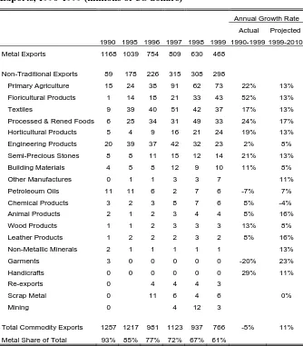
Zambian exports have been dominated by copper. In fact, since Independence and up to 1990, exports consisted almost entirely of copper, which accounted for more that 90 percent of total export earnings. Only recently has diversification into non-traditional exports become important. The details are in Table 4, which reports the evolution and composition of exports from 1990 to 1999. In 1990, metal exports accounted for 93 percent of total commodity exports. Non-traditional exports, such as primary products, agro-processing, and textiles, accounted for the remaining 7 percent. From 1990 to 1999, the decline in metal exports and the increase in non-traditional exports are evident. In 1999, for example, 61 percent of total exports comprised metal products, while 39 percent were non-traditional exports.

Within non-traditional exports, the main components are floriculture products, which increased by 52 percent from 1990 to 1999, processed foods (by 24 percent), primary agricultural products (by 22 percent), horticulture (by 19 percent), Textiles (by 17 percent), and animal products (by 8 percent).

The last column of Table 4 reports some informal export growth projections for some of the non-traditional categories. Notice that agriculture is expected to grow at a high rate over the decade, contributing to nearly 20 percent of total export, up from less than 2 percent in 1990. For COMESA and SADC (Southern Africa Development Community), cotton, tobacco, meat, poultry, dairy products, soya beans, sunflower, sorghum, groundnuts, paprika, maize, and cassava are promising markets. For markets in developed countries (the EU, the US), coffee, paprika, sugar, cotton, tobacco, floriculture, horticulture, vegetables, groundnuts, and honey comprise the best prospects for export growth.

(11)

percent, 15 percent, and 25 percent) with an average rate of around 13 percent. Most tariff lines are ad-valorem (except for a few lines bearing alternative tariffs). No items are subject to seasonal, specific, compound, variable or interim tariffs.

The most common tariff rate is 15 percent, which is applied to around 33 percent of the tariff lines. Almost two thirds of the tariff lines bear a tariff line of either 15 percent or 25 percent, while 21 percent of tariff lines (1,265 lines) are duty-free. These include productive machinery for agriculture, books, and pharmaceutical products. Raw materials and industrial or productive machinery face tariffs in the 0-5 rates. Intermediate goods are generally taxed at a 15 percent rate, and the 25 percent rate is applied to final consumer goods and agricultural-related tariff lines. More concretely, agriculture is the most protected sector, with an average tariff of 18.7 percent, followed by manufacturing, with a 13.2 percent. The average applied MFN tariff in mining and quarrying is 8.2 percent.

Exports are largely liberalized. There are no official export taxes, charges or levies. Further, export controls and regulations are minimal. Maize exports, however, are sometimes subject to bans for national food security reasons. In 2002, for instance, the export ban on maize was in place. There are some export incentives, from tax exemptions to concessions to duty drawback. For example, an income tax of 15 percent (instead of the standard 35 percent rate) is granted to exporters of non-traditional goods who hold an investment license. Also, investments in tourism are sometimes exempted from duties.

III.Non-Traditional Exports and Household Outcomes

We are most interested in exploring the effects of trade on the several outcomes in rural Zambian households. In what follows, we study income gains, and health and educational outcomes.

A. Income

(12)

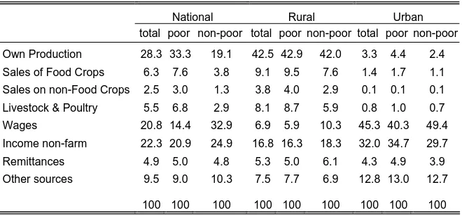
from non-farm businesses (22.3 percent) and wages (20.8 percent). Regarding agricultural income, the sale of Food crops accounts for 6.3 percent of total income, while the sale of Cash crops, for only 2.5 percent. Livestock & Poultry and Remittances account for 5.5 and 4.9 percent of household income, respectively.

There are important differences in income sources between poor and non-poor households. While the share of own-production is 33.3 percent in the average poor household, it is 19.1 percent in non-poor families. In contrast, while wages account for 32.9 percent of the total income of the non-poor, they account for only 14.1 percent of the income of the poor. The shares of the income generated in non-farm businesses are 20.8 and 25 percent in poor and non-poor households respectively. The poor earn a larger share of income from the sales of both food and cash crop, and lower shares from livestock and poultry.

Since we will be looking at the impacts of trade on rural areas, we compare the different sources of income across rural and urban areas. In rural areas, for instance, 42.5 percent of total income is accounted for by own-production; the share in urban areas is only 3.3 percent. The share of non-farm income in rural areas is 16.7 percent, which should be compared with a 32.1 percent in urban areas. In rural areas, the shares from food crops, livestock, wages and cash crops are 9.1, 8.1, 6.9 and 3.8 respectively. In urban areas, in contrast, wages account for 45.3 percent of household income, and the contribution of agricultural activities is much smaller.

The description of income shares is also useful because it highlights the main channels through which trade opportunities can have an impact on household income. We can conclude that, in rural areas, households derive most of their income from subsistence agricultural and non-tradable services (non farm income). Cash crop activities and agricultural wages comprise a smaller fraction of total household income. In our analysis of the differential impacts of trade on household income, we focus on these last farm activities for they are more likely to be directly affected by international markets.6

6

(13)

We explore the poverty alleviation effects of growth in non-traditional exports. If trade leads to higher prices for agricultural goods or higher wages, then there is a first order impact on income given by the income shares described in Table 5. But changes in the extensive margin should be expected, too. In rural areas, this involves farmers switching from subsistence to market-oriented agriculture. For instance, small-scale producers of own-food are expected to benefit from access to markets by producing higher-return cash crops, such as cotton, tobacco, groundnuts or non-traditional exports such as vegetables.

It is this attempt to identify and estimate second round effects of increased market opportunities in rural areas that distinguishes this paper from most of the current literature. Starting with the pioneering work of Deaton (1989) and (1997), estimation of first order effects in consumption and income had become widespread. Techniques to estimate substitution in consumption are also available (Deaton, 1990). But estimation of supply responses has proved much more difficult. The survey in Winters, McCulloch and McKay (2004) highlights these issues and reports some of the available methods and results. In this paper, we capture supply responses using matching methods: by matching households in subsistence agriculture with household in market agriculture, we are able to estimate the average income differential generated by market oriented activities. We do this for different crops as follows.

In rural areas, there are two main channels through which new trade opportunities can affect household income.7 On the one hand, households produce agricultural goods that are sold to agro-processing firms. This involves what we call cash crop activities. On the other hand, household members may earn a wage in a large scale agricultural farm. This means that workers, instead of working in home plots for home production or cash crops, earn a wage in rural (local) labor markets. In this paper, we focus on these two types of activities.

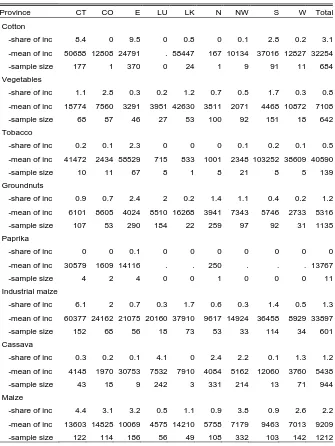
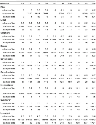
We begin by identifying meaningful agricultural activities for the poverty analysis. Due to regional variation in soil, climate, and infrastructure, the relevant sources of income may be different for households residing in different provinces. To see this, we report in Table 6 the main sources of

7

(14)

household income in the rural areas of the nine Zambian provinces. For each agricultural activity, the table shows the average share of total income accounted for by a given activity, the mean household income conditional on having positive income in a given activity, and the sample size, the number of households that are active in that particular agricultural activity.

Looking at income shares first, we observe that in the Central, Eastern and Southern provinces, the most relevant cash crop activity is cotton. Poultry and Livestock are also important sources of income, particularly in the Southern Province. Tobacco is a promising activity in the Eastern Province, and hybrid maize in the Central province. In the Copperbelt, the most relevant activities are vegetables and hybrid maize; in Luapula, they are groundnuts and cassava; in Northern, cassava and beans; and in North-Western, cassava. In all the provinces, Livestock and Poultry are two good sources of agricultural income.

A key aspect of international trade is that it opens up markets for new products. This implies that some relatively minor sources of income may become quantitatively more important as non-traditional exports grow. Notice, however, that in order to extract meaningful information from the LCMS household survey, we face the practical constraint of sample sizes in our analysis. The data on the number of households reporting positive income and the average value of income for different agricultural activities reported in Table 6 give a sense of the potential relevance of those activities. Based on this information, we identify the following meaningful agricultural activities: cotton, vegetables (including beans), tobacco (in the eastern province only), groundnuts, hybrid maize, cassava, sunflower, and livestock and poultry.

(15)

We perform separate matching exercises, one for each of the cash agricultural activities previously identified in Table 6 (i.e. cotton, tobacco, hybrid maize, groundnuts, vegetables, cassava, sunflower, and rural labor markets).8 We estimate a probit model of participation into market agriculture, which defines the propensity score p(x), for a given vector of observables x. Subsistence farmers are matched with market farmers based on this propensity score, and the income differential is estimated using kernel methods. Details follow.

Let ymh be the income per hectare in market agriculture (e.g. cotton) of household h. Let ysh be the home produced own consumption per hectare. Define an indicator variable M, where M = 1 if the households derive most of their income from cash agriculture. In practice, most Zambian households in rural areas produce something for own consumption. As a consequence, we assign M = 1 to households that derive more than 50 percent of their income from a given cash agricultural activity. Households that derive most of their income from home production are assigned M = 0. The propensity score p(x) is defined as the conditional probability of participating in market agriculture

p(x) = P (M = 1|x) (1) We are interested in estimating the average income differential of those involved in cash market agriculture. This can be defined as

τ

= E [ymh - ysh |M = 1] (2) The main assumption of matching methods is that the participation into market agriculture can be based on observables. This is the ignorability of treatment assignment. More formally, we require that ymh, ysh ⊥ M | x. When the propensity score is balanced, we know that M ⊥ x | p(x). This means that, conditional on p(x), the participation in market agriculture M and the observables x are independent. In other words, observations with a given propensity score have the same distribution of observables x for households involved in market agriculture as in subsistence. The importance of the balancing property, which can be tested, is that it implies that

ymh, ysh⊥ M | p(x) (3)

8

(16)

This means that, conditionally on p(x),the returns in market agriculture and in subsistence are independent of market participation, which implies that households in subsistence and in cash agriculture are comparable.

In general, the assumption that participation depends on observables can be quite strong. In Zambia, the decision to be involved in market agriculture seems to depend on three main variables: access to markets, food security, and tradition in subsistence agriculture. We capture these effects by including in the propensity function several key control variables like regional (district) dummies, the size of the household, the demographic structure of the family, the age and the education of the household head, and the availability of agricultural tools. We believe these variables x comprise a comprehensive set of observables to explain the selection mechanism.

In all our exercises, the balancing condition is tested following the procedure suggested by Dehejia and Whaba (2002). In all the cases, except for paprika and sunflower, the balancing property is satisfied. This is a minor requirement that we impose in our procedure (we cannot test the ignorability requirement). In addition, we graph histograms of the propensity score for those in market and those in subsistence. For the case of cotton, for example, such a plot is reported in Figure 1. We find sufficient overlaps in the propensity scores. Similar results are found in most of the other agricultural activities considered in this paper.

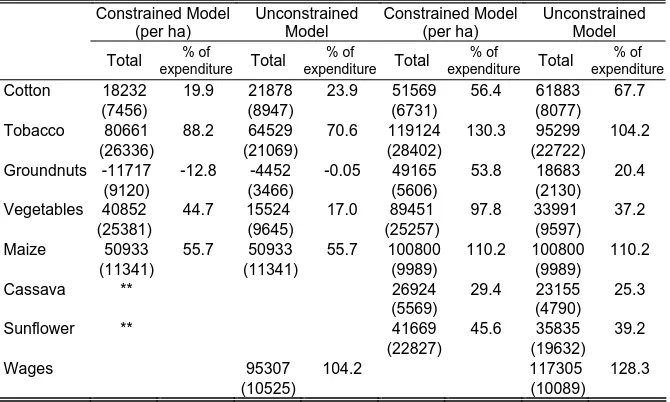
There are two models that we want to explore, the constrained household model and the unconstrained household model. In the latter, households are assumed not to face significant constraints in terms of land, family labor supply, or inputs. This means that it would be possible for the household to plant an additional hectare of, say, cotton or cassava. In this case, the relevant quantity to estimate is the income that could be earned in cash activities. There would be no forgone income by expanding cash crop activities. In contrast, in the constrained household model, land or labor impose a limitation to farming activities. If a family were to plant an additional acre of cotton, then an acre of land devoted to own-consumption (and all other relevant resources) should be released.

(17)

inputs is relatively widespread in the case of cotton due to the outgrower scheme (section II). Other crops, such as hybrid maize, may require purchases of seeds in advance, something that may be difficult for many farmers. Fertilizers may also be expensive, but governmental subsidy programs in place may help ease the constraints. In any case, it is our belief that important lessons can be learnt from the comparison of the results in the two models. The constrained model would give a sense of the short run benefits of moving away from subsistence to market agriculture. The unconstrained model would reveal the additional benefits to Zambian farmers of helping release major agricultural constraints.

Results are reported in Table 7. The first vertical panel corresponds to the gains per hectare in the constrained model. In the second panel, the constrained household is assumed to expand cash agricultural activities by the average size of the plots devoted to each of these activities. The third panel reports the gains per hectare in the unconstrained model; this model is directly comparable to that in the first panel. The last panel reports the gains in the unconstrained model in the hypothetical situation in which the farmer moves from subsistence to market, but devoting the average area to the market crop.

We begin by describing the case of cotton, the major market crop in some provinces. In the constrained model, farmers growing cotton are expected to gain 18,232 kwachas, on average, more than similar farmers engaged in subsistence agriculture. The gain is equivalent to 19.9 percent of the average expenditure of a representative poor farmer. To get a better sense of what these numbers mean, notice that the food poverty line in 1998 was estimated at Kw 32,233 per month and the poverty line, at 46,287 per month (per equivalent adult). Further, since the exchange rate in December 1998 was around 2,200Kw, the gains are equivalent to just over 8 US dollars (in 1998 prices).

(18)

around 2 hectares. This means that, on average, households would be able to substitute away of own-consumption activities and towards cotton growing activities.

Our findings highlight important gains from switching to cotton. However, the magnitudes do not look too high enough, particularly given the relevance of cotton as an export commodity. One explanation for this result is that we have been working with the constrained model, thereby a farmer must forgo income to earn cotton income. If some of these constraints were eliminated, so that households could earn extra income from cotton without giving up subsistence income, gains would be much higher. We estimate these gains with the mean cotton income, conditional on positive income and on being matched with a subsistence farmer.9 The expected gain from planting an additional hectare of cotton would be 51,516 Kw (or approximately 10,273 Kw per equivalent adult). These are larger gains, equivalent to around 56.4 percent of the average expenditure of poor households in rural areas. If the farmer were to grow the average size of cotton crops in Zambia (i.e., 1.2 hectares), then the gains in the unconstrained model would be 61,883 Kw, which is roughly equal to 67.7 percent of the average expenditure of the poor.

Another commercial crop with great potentials in international markets is tobacco. In the constrained model, the gain per hectare of switching from subsistence agriculture to tobacco would be 80,661 monthly kwachas, or roughly 88.2 percent of average total household expenditure. Since, on average, 0.8 hectares are allocated to tobacco, the household would gain 64,529 Kwachas if this plot size were planted. In the unconstrained model, the gain would be 119,124 Kw, around 130 percent of the total expenditure of an average poor household. If the average of 0.8 hectares were planted (without any constrains), the income gains would reach 95,299 Kw, approximately doubling expenditure. Growing tobacco seems to be an important vehicle for poverty alleviation.

Results for vegetables and groundnuts, two activities often mentioned as good prospects for non-traditional exports, reveal that no statistically significant gains can be expected in the constrained model. In the data, there is

9

(19)

evidence of higher earnings in planting vegetables and lower earnings in planting groundnuts but neither are statistically significant. Instead, gains can be realized if the constrains are released. For vegetables, the gain per hectare would be 89,451 Kw, or 33,991 Kw if the average plot size devoted to this crop is planted. This is 37,2 percent of total average household expenditure. In the case of groundnuts, these gains would be equivalent to only 20 percent of the expenditure of households in poverty.

One key crop in Zambia is maize, which is grown by the vast majority of households. Farmers grow local varieties and hybrid maize. The former is mainly devoted to own-consumption and is not considered suitable for world markets. Hybrid maize is, instead, potentially exportable. In Table 7, we find that a farmer that switches from purely subsistence activities to produce (and sell) hybrid maize would make 50,933 additional kwachas. This gain, which is statistically significant, is equivalent to 55.7 percent of the expenditure of the poor. This is the expected gain, on average, since the average plot allocated to hybrid maize is estimated at precisely 1 hectare. If we assume that an additional hectare of maize is planted in a model without household constraints, the income differential would be 100,800 kwachas or around the average expenditure of poor households.

These are important results. To begin with, we find support for the argument that claims that income gains can be achieved through the production and sale of hybrid maize. In addition, since most Zambian farmers across the whole country grow (or grew) maize, there is a presumption that they are able to produce it efficiently and that some of the constraints faced in other crops may not be present. Know-how, fertilizer use, seeds usage, are examples. In those regions in which cotton and tobacco, major exportable crops, are not suitable agricultural activities (due to weather or soil conditions), the production of hybrid maize appears as a valid alternative.

(20)

investments. In addition, disease control is critical in these activities, and it is unclear whether Zambia will manage to achieve the standards needed to compete in international markets.

There is an additional exercise that we perform. If larger market access is achieved, rural labor markets may expand and workers may become employed and earn a wage. We can learn about the magnitudes of the income gains of moving from home plot agriculture to rural wage employment in agriculture by comparing the average income obtained in these activities. Concretely, we compare the average monthly wages of those workers employed in rural labor markets with the own-consumption per working household member in subsistence agriculture.10 In Table 7, we estimate again of 95,307 Kw per month in the constrained model (so that individuals would have to leave farming activities at home to work at a local large farm). In the unconstrained model (i.e., a model in which the worker becomes employed but keeps working in subsistence during the weekends), the gains would be 117,305 Kw. These gains range from 104.2 percent to 128.3 percent of the total expenditure of the average poor household in rural areas.

As in the cases of cotton, tobacco, and maize, the magnitudes of these gains suggest that rural employment in commercial farms could be good instruments for poverty alleviation. By fostering the development of larger scale agricultural activities, there is evidence that international trade opportunities can help rural farmers to move out of poverty through rural labor markets, employment and wage income.

An important element for these results to become feasible is the role of complementary policies. Access to international markets is a basic prerequisite. This requires openness and export oriented incentives on behalf of Zambia, but also a liberalization of agricultural markets in developed countries. Subsidies to cotton, for instance, which are widespread and cause prices to be lower than market prices, should be eliminated. But other domestic complementary policies should be implemented as well. We identify several key policies. Extension services to farmers, including transmission of information and know-how about cropping, crop diversification, fertilizer and pesticide use, etc., are critical. The provision of infrastructure to reduce transport and transaction costs is also essential. Irrigation may also help. The

10_{This is computed as the ratio of reported own-consumption and the total number of household}

(21)

development of a stronger financial and credit markets can also help farmers reduce the costs of the outgrower programs. Finally, education (both formal education and labor discipline) and the provision of better health services will surely help increase farm productivity in market agriculture.

B. Anthropometry and Education

In this section, we focus on the non-monetary effects of market agriculture. We look at the effects on two household outcomes, namely the nutritional status of infants and young children (from 0 to 60 months old) and education performance of children in primary and secondary school.

Malnutrition remains a widespread problem in developing countries as does in Zambia. We assess the nutritional status on the basis of anthropometric indicators (such as height or weight). We analize the three most commonly used anthropometric indicators for infants and children: weight-for-age, height-for-age, and weight-for-height.

Weight-for-height (whz) measures body weight relative to height. It is normally used as an indicator of current nutritional status, and can be useful for measuring short-term changes in nutritional status. Extreme cases of low whz relative to a child of the same sex and age in a reference population are commonly referred to as “wasting”. Wasting may be the consequence of starvation or severe disease (in particular diarrhea), but it can also be due to chronic conditions. Height-for-age (haz) reflects cumulative linear growth. haz deficits indicate past or chronic inadequacies nutrition and/or chronic or frequent illness, but cannot measure short-term changes in malnutrition. Extreme cases of low haz are referred to as “stunting''. Weight-for-age (waz) reflects body mass relative to age. This is, in effect, a composite measure of height-for-age and weight-for-height, making interpretation difficult. The term “underweight” is commonly used to refer to severe or pathological deficits in waz.

(22)

(standard deviation scores) which is the most common way of expressing anthropometric indices.11 Table 8 presents some summary statistics.

The value of the mean of the haz z-score is -2.21, reflecting long-term cumulative inadequacies of health and/or nutrition.12 There seems to be no wasting problem, the mean of whz is 0.23. Using the summary measure of nutritional status (waz) there is mild underweight, probably caused by long-term nutritional problems.

For the education outcome, we generated an index of school performance for children between ages 7 and 18, that is, children in primary and secondary school. The index is the ratio of years of education completed by an individual and the years of education this individual should have for her age.13 The mean of this index for rural areas is 0.49 including children not attending school (approximately 45% of the sample).

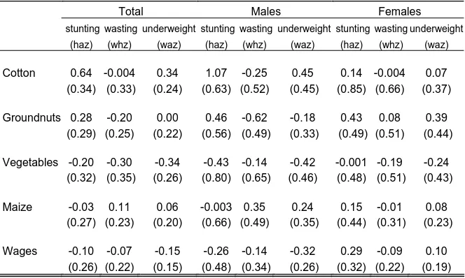
We now describe the exercises performed using the same matching methods as in the previous section. We wanted to assess the effects of market agriculture in other dimensions than monetary income. Then, for the same cash crops and wage employment in Table 7, we estimated the effects on child nutrition and education of a switching from subsistence to market agriculture. Table 9 reports the effects on child nutrition and Table 10 on education. Due to data limitations, exercises on tobacco, cassava and sunflower were not feasible.

There are three vertical panels in Table 9. The first correspond to the sample of all infants and young children (0 to 59 months old), the second to a subsample of males, and the third to females. We found no effect on nutrition for none of the crops except for a long-run gain in the case of cotton. The effect on haz for those switching to cotton would be an increase of 0.64 in the z-score, equivalent to 30 percent of the average haz z-score for households in subsistence. There is no differential effect between females and males,

11

A z-score is defined as the difference between the value for an individual and the median value of the reference population for the same age or height, divided by the standard deviation of the reference population.

12

The WHO uses a z-score cut-off point of -2 to classify low weight-for-age, low height-for-age and low weight-for-height as moderate and severe undernutrition, and –3 to define severe undernutrition.

13

(23)

although the magnitudes for boys tend to be much higher than for girls (and they are marginally significant, too).

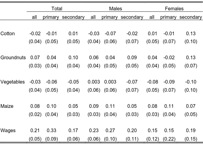
In Table 10 we report the effects on education for children between 7 and 18 years old. The first panel includes the effect for the total sample and for those children between ages 7 and 13 (primary school) and between 14 and 18 (secondary school). The second panel is only for males and the third only for females. We found positive effects on education performance in the cases of groundnuts and maize and a larger effect in the case of wages. The effect of wage employment is 0.21, which is equivalent to 60 percent of the average index for individuals in subsistence agriculture. The effects of groundnuts and maize are 0.07 and 0.08 respectively, representing 20 and 23 percent of the average index. There is no significant effect for cotton and vegetables. There seems to be a larger effect on males than on females, and on primary school than on secondary.

IV.Conclusions

In this paper, we have investigated some of the impacts of international trade and economic reforms on rural households in Zambia. This is a low income country, with widespread and prevalent poverty at the national and regional levels. In rural areas, poverty is still higher. In this context, efforts devoted to find ways to alleviate poverty should be welcome. In Zambia, the government and international institutions have long been actively searching for programs and policies to improve the living standards of the population. Concretely, a set of reforms were implemented during the 1990s, including liberalization, privatization, and deregulation of marketing boards in agriculture. Further, farmers and firms were encouraged to look more closely at international markets.

After episodes of economic reforms, households are affected both as consumers and as income earners. Non-monetary outcomes can also be affected. We have looked at several aspects of the globalization-poverty link. On the income side, we have estimated income gains from market agriculture vis-a-vis subsistence agriculture. On non-monetary outcomes, we have investigated differences in nutritional and educational status of Zambian children.

(24)

tobacco, hybrid maize, vegetables, and groundnuts. Further, by raising the demand for rural labor, rural wages would increase as well. Our results indicate that rural Zambians would gain substantially from expanding world markets, particularly in terms of cotton, tobacco and maize income as well as of wages.

Results on non-monetary outcomes are mixed. Some crops, like cotton, affect long-run nutritional status but show no effect of wasting or educational status. Other major agricultural activities, like wages, maize or groundnuts, affect educational outcomes but show no effect on nutritional status. Interestingly, there seems to be larger effects on boys than on girls, and on primary school than on secondary schooling.

(25)

References

Barnum, H., and L. Squire (1979). “A model of an Agricultural Household. Theory and Evidence.” World Bank Ocassional Papers No 27.

Benjamin, D. (1992). “Household Composition, Labor Markets, and Labor Demand: Testing for Separation in Agricultural Household Models.” Econometrica, Vol. 60: 287-322.

Cotton News (2002). Cotton Development Trust, Zambia.

Deaton, A. (1989). “Rice Prices and Income Distribution in Thailand: a Non-Parametric Analysis.” Economic Journal, Vol. 99: 1-37.

Deaton, A. (1990). “Price Elasticities from Survey Data.” Journal of Econometrics, Vol. 44: 281-309.

Deaton, A. (1997). The Analysis of Household Surveys. A Microeconometric

Approach to Development Policy. John Hopkins University Press for the

World Bank.

Dehejia, R., and S. Wahba (2002). “Propensity Score Matching Methods for Non-Experimental Causal Studies.” Review of Economic Studies, Vol. 84 (1): 151-161.

Fan, J. (1992). “Design-adaptive nonparametric regression.” Journal of the American Statistical Association, Vol. 87 (420): 998-1004.

Feenstra, R.C. (2003). Advanced International Trade: Theory and Evidence. Forthcoming. Princeton: Princeton University Press.

Food Security Research Project (2000). “Improving Smallholder and Agribusiness Opportunities in Zambia's Cotton Sector: Key Challenges and Options.” Working Paper No 1, Lusaka, Zambia.

(26)

Heckman, J., H. Ichimura, and P. Todd (1997). “Matching as an Econometric Evaluation Estimator: Evidence from Evaluating a Job Training Programme.” Review of Economic Studies, Vol. 64 (4): 605-654.

Heckman, J., H. Ichimura, and P. Todd (1998). “Matching as an Econometric Evaluation Estimator.” Review of Economic Studies, Vol. 65 (2): 261-294.

Lalonde, R. (1986). “Evaluating the Econometric Evaluations of Training Programs.” American Economic Review, Vol. 76(4): 604-620.

Litchfield, J. and N. McCulloch (2003). “Poverty in Zambia: Assessing the Impacts of Trade Liberalization in the 1990s.” Mimeo, Poverty Research Unit, Sussex University.

McCulloch, N., B. Baulch, and M. Cherel-Robson (2001). “Poverty, Inequality and Growth in Zambia During the 1990s”, presented at WIDER Development Conference, Helsinski, May 2001.

Mwiinga, W., J. Nijhoff, T. Jayne, G. Tembo and J. Shaffer (2002). “The Role of Mugaiwa in Promoting Household Food Security.” Policy Synthesis No 5, Food Security Research Project, Zambia.

Pagan, A. and A. Ullah (1999). Nonparametric Econometrics. New York: Cambridge University Press.

Porto, G. (2004). “Informal Export Barriers and Poverty.” Journal of International Economics, forthcoming.

Rosenbaum, P., and D. Rubin (1983). “The Central Role of the Propensity Score in Observational Studies of Causal Effects.” Biometrika, Vol. 70(1): 41-55.

Rubin, D. (1977). “Assignment to a Treatment Group on the Basis of a Covariate.” Journal of Educational Statistics, Vol. 2(1): 1-26.

Singh, I., L. Squire, and J. Strauss, eds. (1986). Agricultural Household

Models: Extensions, Applications and Policy. Baltimore: Johns Hopkins

University Press for the World Bank.

(27)

(28)

[image:28.595.135.453.217.278.2]

Table 1

Poverty in Zambia (head count)

1991 1996 1998

National 69.6 80.0 71.5

Rural 88.3 90.5 82.1

Urban 47.2 62.1 53.4

Note: The head count is the percentage of the population below the poverty line. Own calculations based on Priority Survey (1991), Living Conditions Monitoring Survey (1996) and Living Conditions Monitoring Survey (1998).

Table 2

Poverty Profile in 1998 (head count)

total rural urban

National 71.5 82.1 53.4

Central 74.9 82.3 60.5

Copperbelt 63.2 82.1 57.5

Eastern 79.1 80.6 64.4

Luapula 80.1 84.6 52.4

Lusaka 48.4 75.7 42.4

Northern 80.6 83.3 66.4

North-Western 74.3 77.4 54.1

Southern 68.2 73.0 51.8

Western 88.1 90.3 69.5

[image:28.595.139.453.361.530.2]

(29)

[image:29.595.139.465.216.655.2]

Table 3

Major Economic Reforms. Zambia 1989-1998

Stabilization Policy Agricultural Price Parastatal Reform

Year

and Key Events and Marketing

Trade Reforms

_{and Privatization}

1989 Decontrol of all con- Abolition of national sumer prices (except maize marketing

maize). board.

1990 Policy Framework Pa- Demonopolization of

per agreed with IMF. agricultural marketing;

maize meal subsidy

withdrawn.

1991 IMF suspends dis- Removal of most ex-

bursements in June. port controls; removal Inflation soars. Elec- of ban on maize ex-

tion of MMD in ports.

October.

1992 Introduction of Trea- Severe drought; re- Simplication and sury Bill Financing; moval of mealie meal compression of tariff decontrol of borrow- subsidy; removal of rates; increase in the ing and lending rates; fertilizer subsidy. tariff preference for introduction of "bu- goods from COMESA. reau de change” for

exchange rate deter-

mination.

1993 Introduction of cash Failed attempt to re- Privatization act

budgeting. form agricultural mar- passed; Zambia Pri-

keting. vatization Agency

formed

1994 Capital account liber- Launch of the Agricul-

alization. tural Credit Manage-

ment Programme.

1995 Privatization of the Removal of 20 percent Dissolution of the milling industry; uplift factor applied to Zambia Industria and

launch of WB agricul- import values. Minning Corportation

tural sector investment (ZIMCO).

(30)

Table 3 (continued)

Stabilization Policy Agricultural Price Parastatal Reform

Year

and Key Events and Marketing

Trade Reforms

and Privatization

1996 MMD win elections Acceleration of privati-

but UNIP boycott zation programme.

elections.

1997 Donors withdraw bal-

ance of payment sup-

port.

1998 Copper prices ad- Negotiations on Zam-

versely affected by bia Consolidated Cop-

East Asian crisis. per Mines (ZCCM) sale

fall through.

[image:30.595.137.467.205.361.2]

(31)

[image:31.595.138.472.206.587.2]

Table 4

Exports, 1990-1999 (millions of US dollars)

Annual Growth Rate

Actual Projected

1990 1995 1996 1997 1998 1999 1990-1999 1999-2010

Metal Exports 1168 1039 754 809 630 468

Non-Traditional Exports 89 178 226 315 308 298

Primary Agriculture 15 24 38 91 62 73 22% 13%

Floricultural Products 1 14 18 21 33 43 52% 13%

Textiles 9 39 40 51 42 37 17% 13%

Processed & Rened Foods 6 25 34 31 49 33 24% 17%

Horticultural Products 5 4 9 16 21 24 19% 13%

Engineering Products 20 39 37 42 32 23 2% 8%

Semi-Precious Stones 8 8 11 15 12 14 21% 13%

Building Materials 4 5 8 12 9 10 11% 8%

Other Manufactures 0 1 1 3 3 7 11%

Petroleoum Oils 11 11 6 2 7 6 -7% 7%

Chemical Products 3 2 3 8 7 6 8% -4%

Animal Products 2 1 2 3 4 4 8% 16%

Wood Products 1 1 2 3 3 3 13% 8%

Leather Products 1 2 2 2 3 2 8% 16%

Non-Metallic Minerals 2 1 1 1 1 1 13%

Garments 3 0 0 0 0 0 -20% 23%

Handicrafts 0 0 0 0 0 0 29% 11%

Re-exports 0 4 4 4 3

Scrap Metal 0 11 6 4 6 0%

Mining 0 4 12 3

Total Commodity Exports 1257 1217 981 1123 937 766 -5% 11%

Metal Share of Total 93% 85% 77% 72% 67% 61%

(32)

[image:32.595.138.468.219.373.2]

Table 5

Sources of Income (percentage)

National Rural Urban

total poor non-poor total poor non-poor total poor non-poor

Own Production 28.3 33.3 19.1 42.5 42.9 42.0 3.3 4.4 2.4

Sales of Food Crops 6.3 7.6 3.8 9.1 9.5 7.6 1.4 1.7 1.1

Sales on non-Food Crops 2.5 3.0 1.3 3.8 4.0 2.9 0.1 0.1 0.1

Livestock & Poultry 5.5 6.8 2.9 8.1 8.7 5.9 0.8 1.0 0.7

Wages 20.8 14.4 32.9 6.9 5.9 10.3 45.3 40.3 49.4

Income non-farm 22.3 20.9 24.9 16.8 16.3 18.3 32.0 34.7 29.7

Remittances 4.9 5.0 4.8 5.3 5.0 6.1 4.3 4.9 3.9

Other sources 9.5 9.0 10.3 7.5 7.7 6.9 12.8 13.0 12.7

100 100 100 100 100 100 100 100 100

(33)

[image:33.595.138.473.212.658.2]

Table 6

Income Shares, Average Income and Sample Sizes

Province CT CO E LU LK N NW S W Total

Cotton

-share of inc 8.4 0 9.5 0 0.8 0 0.1 2.8 0.2 3.1

-mean of inc 50688 12808 24791 . 58447 167 10134 37016 12827 32254

-sample size 177 1 370 0 24 1 9 91 11 684

Vegetables

-share of inc 1.1 2.8 0.3 0.2 1.2 0.7 0.5 1.7 0.3 0.8

-mean of inc 18774 7560 3291 3951 42630 3811 2071 4468 10872 7108

-sample size 68 87 46 27 53 100 92 151 18 642

Tobacco

-share of inc 0.2 0.1 2.3 0 0 0 0.1 0.2 0.1 0.5

-mean of inc 41472 2434 58529 715 833 1001 2348 103252 38609 40590

-sample size 10 11 67 8 1 8 21 8 5 139

Groundnuts

-share of inc 0.9 0.7 2.4 2 0.2 1.4 1.1 0.4 0.2 1.2

-mean of inc 6101 8605 4024 8510 16268 3941 7343 5746 2733 5316

-sample size 107 53 290 184 22 259 97 92 31 1135

Paprika

-share of inc 0 0 0.1 0 0 0 0 0 0 0

-mean of inc 30579 1609 14116 . . 250 . . . 13767

-sample size 4 2 4 0 0 1 0 0 0 11

Industrial maize

-share of inc 6.1 2 0.7 0.3 1.7 0.6 0.3 1.4 0.5 1.3

-mean of inc 60377 24162 21075 20160 37910 9617 14924 36458 8929 33897

-sample size 152 68 56 18 73 53 33 114 34 601

Cassava

-share of inc 0.3 0.2 0.1 4.1 0 2.4 2.2 0.1 1.3 1.2

-mean of inc 4148 1970 30753 7532 7910 4084 5162 12060 3760 5438

-sample size 43 18 9 242 3 331 214 13 71 944

Maize

-share of inc 4.4 3.1 3.2 0.5 1.1 0.9 3.8 0.9 2.6 2.2

-mean of inc 13603 14825 10069 4575 14210 5758 7179 9463 7013 9209

(34)

Rice

-share of inc 0 0 0.3 0.1 0 0.1 0 0 1.2 0.2

-mean of inc . 1250 4614 6664 . 3884 1502 . 8040 5762

-sample size 0 1 39 9 0 31 3 0 48 131

Millet

-share of inc 0.9 0.1 0.2 0.3 0 1.3 0 0 0.2 0.4

-mean of inc 4821 1402 4253 2338 . 2727 1574 2250 3161 2965

-sample size 26 12 29 48 0 222 7 1 33 378

Sorghum

-share of inc 0.1 0.2 0 0 0.1 0.2 0.5 0 0.2 0.1

-mean of inc 3409 5220 838 1209 35209 1938 4473 0 3002 3166

-sample size 17 17 4 12 5 45 60 1 16 177

Beans

-share of inc 0.2 0.1 0 0.5 0 2 0.8 0 0 0.5

-mean of inc 6486 1922 6388 9668 8631 11007 3679 2679 2412 8598

-sample size 18 17 12 49 2 219 95 8 3 423

Soya beans

-share of inc 0.4 0 0.4 0.1 0 0 0 0 0 0.1

-mean of inc 26102 3611 6277 6250 5427 3958 868 652 . 10989

-sample size 19 3 30 1 2 6 2 2 0 65

Sweet potatoe

-share of inc 0.9 2.8 0.1 1 0 0.3 1.6 0.1 0.5 0.7

-mean of inc 5827 5547 2800 1820 1746 2082 3841 2546 5292 3658

-sample size 57 154 26 110 9 124 159 29 29 697

Irish potatoe

-share of inc 0 0.1 0 0.1 0 0 0.3 0.1 0 0.1

-mean of inc 9987 8935 2494 5810 333333 2443 4321 25420 . 8135

-sample size 5 6 7 6 1 6 31 13 0 75

Sunflower

-share of inc 0.1 0 0.5 0 0 0.1 0.1 0.2 0 0.1

-mean of inc 12656 4167 4834 750 7738 3424 1100 5770 . 5472

-sample size 17 1 38 1 4 13 5 45 0 124

Livestock

-share of inc 2.9 1.3 4.3 0.6 3.8 2 2.3 8 6.9 3.8

-mean of inc 16126 11606 11910 11808 14285 8701 12955 44612 14936 19442

[image:34.595.138.474.200.636.2]

(35)

Poultry

-share of inc 6.4 2.2 4.5 2.7 5.9 3.4 2.8 4.6 6.7 4.3

-mean of inc 3329 6530 2550 2061 5967 1940 2220 3762 1501 2778

-sample size 476 228 766 476 291 731 510 637 365 4480

[image:35.595.137.473.205.271.2]

Note: CT: Central; CO: Copperbelt; E: Eastern; LU: Luapula; LK: Lusaka; N: Northern; NW: Northwestern; S: Southern; W: Western. Income shares are in percentage and mean of income in monthly Kwachas. Own calculations based on Living Conditions Monitoring Survey (1998).

Table 7

Income Gains from Market Agriculture

Constrained Model Constrained Model

(per ha)

Unconstrained

Model (per ha)

Unconstrained Model

% of % of % of % of

Total

expenditure Total expenditure Total expenditure Total expenditure Cotton 18232 19.9 21878 23.9 51569 56.4 61883 67.7

(7456) (8947) (6731) (8077)

Tobacco 80661 88.2 64529 70.6 119124 130.3 95299 104.2

(26336) (21069) (28402) (22722)

Groundnuts -11717 -12.8 -4452 -0.05 49165 53.8 18683 20.4

(9120) (3466) (5606) (2130)

Vegetables 40852 44.7 15524 17.0 89451 97.8 33991 37.2

(25381) (9645) (25257) (9597)

Maize 50933 55.7 50933 55.7 100800 110.2 100800 110.2

(11341) (11341) (9989) (9989)

Cassava ** 26924 29.4 23155 25.3

(5569) (4790)

Sunflower ** 41669 45.6 35835 39.2

(22827) (19632)

Wages 95307 104.2 117305 128.3

(10525) (10089)

[image:35.595.138.473.360.561.2]

(36)

[image:36.595.135.473.216.287.2]

Table 8

Child Nutrition in Rural Areas (0 to 59 months old)

z-score Prevalence rates

mean sd moderate severe

stunting (haz) -2.21 1.77 23% 33% wasting (whz) 0.23 1.40 5% 1% underweight (waz) -1.21 1.24 20% 6%

[image:36.595.138.470.401.600.2]

Note: Height-for-age (haz) is a measure of accumulated undernutrition. Weight-for-height (whz) is used to measure levels of current undernutrition. Weight-for-age (waz) is used as a summary measure of nutritional status. In medicine, the prevalence rate is the proportion of individuals suffering a disease. Moderate refers to those individuals with a z-score between -3 and -2, and severe refers to a z-score below -3.

Table 9

Effects on Child Nutrition from Market Agriculture (0 to 59 months old)

Total Males Females

stunting wasting underweight stunting wasting underweight stunting wasting underweight (haz) (whz) (waz) (haz) (whz) (waz) (haz) (whz) (waz)

Cotton 0.64 -0.004 0.34 1.07 -0.25 0.45 0.14 -0.004 0.07

(0.34) (0.33) (0.24) (0.63) (0.52) (0.45) (0.85) (0.66) (0.37)

Groundnuts 0.28 -0.20 0.00 0.46 -0.62 -0.18 0.43 0.08 0.39

(0.29) (0.25) (0.22) (0.56) (0.49) (0.33) (0.49) (0.51) (0.44)

Vegetables -0.20 -0.30 -0.34 -0.43 -0.14 -0.42 -0.001 -0.19 -0.24

(0.32) (0.35) (0.26) (0.80) (0.65) (0.46) (0.48) (0.51) (0.43)

Maize -0.03 0.11 0.06 -0.003 0.35 0.24 0.15 -0.01 0.08

(0.27) (0.23) (0.20) (0.66) (0.49) (0.35) (0.44) (0.31) (0.23)