Automatic source detection in astronomical images

Texto completo

(1)AUTOMATIC SOURCE DETECTION IN ASTRONOMICAL IMAGES Marc MASIAS MOYSET. Dipòsit legal: Gi. 1373-2014 http://hdl.handle.net/10803/275990. ADVERTIMENT. L'accés als continguts d'aquesta tesi doctoral i la seva utilització ha de respectar els drets de la persona autora. Pot ser utilitzada per a consulta o estudi personal, així com en activitats o materials d'investigació i docència en els termes establerts a l'art. 32 del Text Refós de la Llei de Propietat Intel·lectual (RDL 1/1996). Per altres utilitzacions es requereix l'autorització prèvia i expressa de la persona autora. En qualsevol cas, en la utilització dels seus continguts caldrà indicar de forma clara el nom i cognoms de la persona autora i el títol de la tesi doctoral. No s'autoritza la seva reproducció o altres formes d'explotació efectuades amb finalitats de lucre ni la seva comunicació pública des d'un lloc aliè al servei TDX. Tampoc s'autoritza la presentació del seu contingut en una finestra o marc aliè a TDX (framing). Aquesta reserva de drets afecta tant als continguts de la tesi com als seus resums i índexs.. ADVERTENCIA. El acceso a los contenidos de esta tesis doctoral y su utilización debe respetar los derechos de la persona autora. Puede ser utilizada para consulta o estudio personal, así como en actividades o materiales de investigación y docencia en los términos establecidos en el art. 32 del Texto Refundido de la Ley de Propiedad Intelectual (RDL 1/1996). Para otros usos se requiere la autorización previa y expresa de la persona autora. En cualquier caso, en la utilización de sus contenidos se deberá indicar de forma clara el nombre y apellidos de la persona autora y el título de la tesis doctoral. No se autoriza su reproducción u otras formas de explotación efectuadas con fines lucrativos ni su comunicación pública desde un sitio ajeno al servicio TDR. Tampoco se autoriza la presentación de su contenido en una ventana o marco ajeno a TDR (framing). Esta reserva de derechos afecta tanto al contenido de la tesis como a sus resúmenes e índices.. WARNING. Access to the contents of this doctoral thesis and its use must respect the rights of the author. It can be used for reference or private study, as well as research and learning activities or materials in the terms established by the 32nd article of the Spanish Consolidated Copyright Act (RDL 1/1996). Express and previous authorization of the author is required for any other uses. In any case, when using its content, full name of the author and title of the thesis must be clearly indicated. Reproduction or other forms of for profit use or public communication from outside TDX service is not allowed. Presentation of its content in a window or frame external to TDX (framing) is not authorized either. These rights affect both the content of the thesis and its abstracts and indexes..

(2) PhD Thesis. Automatic source detection in astronomical images. Marc Masias Moyset. 2014.

(3)

(4) PhD Thesis. Automatic source detection in astronomical images. Marc Masias Moyset. 2014. Doctoral Programme in Technology. Supervised by: Jordi Freixenet, Marta Peracaula and Xavier Lladó. Work submitted to the University of Girona in partial fulfilment of the requirements for the degree of Doctor of Philosophy.

(5)

(6) Publications Journals • [A&C 2014] M. Masias, X. Lladó, M. Peracaula and J. Freixenet. “Multiscale distilled sensing: astronomical source detection in long wavelength images”. Astronomy and Computing, submitted. • [NewA 2014] M. Peracaula, A. Torrent, M. Masias, X. Lladó, J. Freixenet, J. Martı́, J.R. Sánchez-Sutil, A.J. Muñoz-Arjonilla and J.M. Paredes. “Exploring three faint source detections methods for aperture synthesis radio images”. New Astronomy, submitted. • [ExA 2013] M. Masias, M. Peracaula, J. Freixenet and X. Lladó. “A quantitative analysis of source detection approaches in optical, infrared, and radio astronomical images”. Experimental Astronomy, 36(3), pp. 591-629. 2013. • [MNRAS 2012] M. Masias, J. Freixenet, X. Lladó and M. Peracaula. “A review of source detection approaches in astronomical images”. Monthly Notices of the Royal Astronomical Society, 422(2), pp. 1674-1689. 2012.. Conferences • [ADASS 2013] M. Masias, J. Freixenet, M. Peracaula and X. Lladṕ. “Multiscale source detection for long wavelength astronomical images”. 23rd International Conference on Astronomical Data Analysis Software and Systems. ASP Conference Series, to appear. Waikoloa, Hawaii, USA. October 2013. • [ICIP 2013] M. Masias, X. Lladó, M. Peracaula and J. Freixenet. “Multiscale distilled sensing: a source detection method for infrared and radio astronomical i.

(7) images”. 2013 IEEE International Conference on Image Processing. ICIP 2013 Proceedings, pp. 2378-2382. Melbourne, Australia. September 2013. • [ADASS 2011] M. Masias, J. Freixenet, X. Lladó and M. Peracaula. ”Quantitative evaluation of source detection strategies in astronomical images”. 21st International Conference on Astronomical Data Analysis Software and Systems. ASP Conference Series, 461, pp. 793-796. Paris, France. November 2011.. ii.

(8) List of Acronyms AIPS Astronomical Image Processing System ALMA Atacama Large Millimeter/submillimeter Array ATCA Australia Telescope Compact Array CCD Charge-Coupled Device CGPS Canadian Galactic Plane Survey CRT Continuous Ridgelet Transform CC-trees Connected Component trees Dec Declination DS Distilled Sensing ESD Extended Source Detection FDR False Discovery Rate FITS Flexible Image Transport System FN False Negative FP False Positive FSD Faint Source Detection FWHM Full Width at Half Maximum GALEX Galaxy Evolution Explorer GMRT Giant Metrewave Radio Telescope iii.

(9) GN González-Nuevo HDU Header and Data Units HST Hubble Space Telescope INTEGRAL INTErnational Gamma-Ray Astrophysics Laboratory ISO Infrared Space Observatory MAP Maximum-A-Posteriori MCMC Markov-Chain Monte Carlo MDS Multiscale Distilled Sensing MF Matched Filter MHWF Mexican Hat Wavelet Family MHWT Mexican Hat Wavelet Transform MSVST Multiscale Variance Stabilisation Transform MVM Multiscale Vision Model NVSS NRAO VLA Sky Survey PCA Principal Component Analysis PCA-NN Principal Component Analysis Neural Networks PDS Phoenix Deep Survey PRF Point Response Function PSD Point Source Detection PSF Point Spread Function RA Right Ascension RCF Radial Contrast Function SAD Search And Destroy SD Source Detection iv.

(10) SDSS Sloan Digital Sky Survey SE Structural Element SKA Square Kilometre Array SNR Signal-to-Noise Ratio SOFIA Stratospheric Observatory For Infrared Astronomy SWT Stationary Wavelet Transform TN True Negative TP True Positive TSD True Sources Detected VICOROB Computer Vision and Robotics WALT Wavelets And Local Thresholding WISE Wide-field Infrared Survey Explorer WT Wavelet Transform XMM-Newton X-ray Multi-Mirror Mission-Newton. v.

(11) vi.

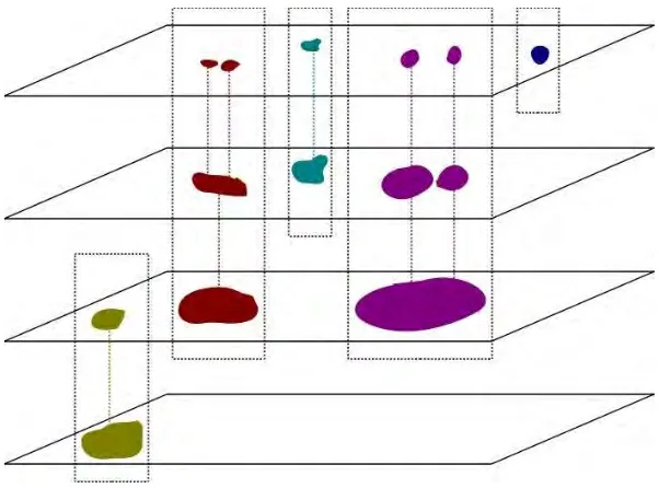
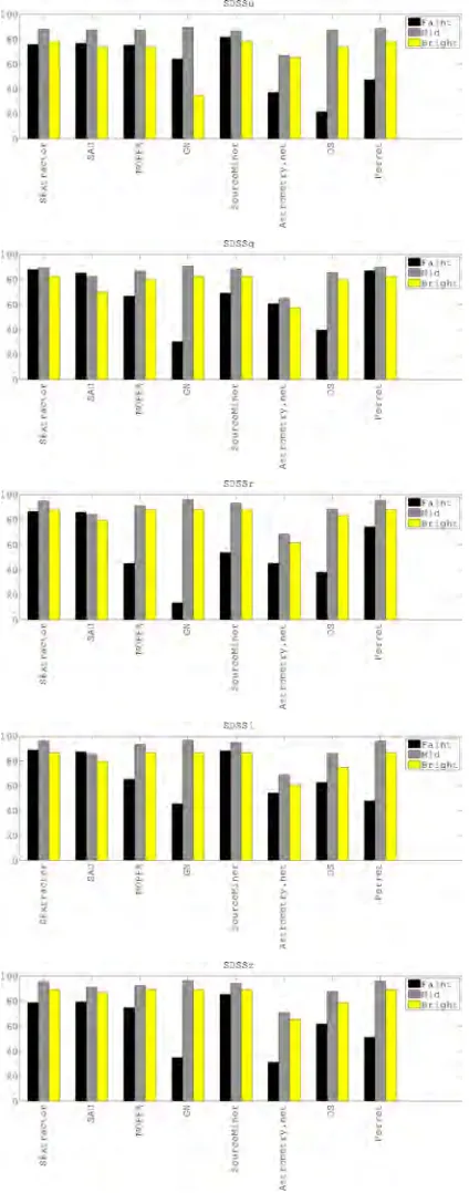
(12) List of Figures 1.1. Electromagnetic spectrum. . . . . . . . . . . . . . . . . . . . . . . . . . . . .. 3. 1.2. Two examples of telescopes . . . . . . . . . . . . . . . . . . . . . . . . . . .. 4. 1.3. Some examples of astronomical objects . . . . . . . . . . . . . . . . . . . . .. 8. 1.4. Graphical representation of the effect of the PSF in images. . . . . . . . . .. 9. 1.5. Radio image with different contrast stretching . . . . . . . . . . . . . . . . .. 9. 1.6. An infrared mosaic with background variations . . . . . . . . . . . . . . . . 11. 2.1. Wavelet decomposition of an image in several scales . . . . . . . . . . . . . 29. 2.2. Example of the connectivity in the wavelet scales. . . . . . . . . . . . . . . . 36. 2.3. Simple graphical example to explain TP, FP, FN, and TN measures . . . . 41. 3.1. The three datasets. . . . . . . . . . . . . . . . . . . . . . . . . . . . . . . . . 59. 3.2. The three datasets with some problematic regions excluded . . . . . . . . . 62. 3.3. Graphical representation of the TP and TSD of the different methods in the three different datasets. . . . . . . . . . . . . . . . . . . . . . . . . . . . 73. 3.4. Graphical representation of the percentages of TSD in the optical dataset according to the brightness of the sources.. 3.5. . . . . . . . . . . . . . . . . . . 74. Graphical representation of the percentages of TSD in the infrared dataset according to the brightness of the sources. . . . . . . . . . . . . . . . . . . . 75. 3.6. Graphical representation of the percentages of TSD in the radio dataset according to the brightness of the sources.. 4.1. . . . . . . . . . . . . . . . . . . 76. Decomposition of an image in 6 scales . . . . . . . . . . . . . . . . . . . . . 86 vii.

(13) 4.2. Graphical representation of the first algorithm (WALT) . . . . . . . . . . . 87. 4.3. Graphical representation of the second algorithm (RCF) . . . . . . . . . . . 89. 4.4. Graphical representation of the third algorithm (the boosting classifier) . . 91. 4.5. Dictionary building process. . . . . . . . . . . . . . . . . . . . . . . . . . . . 92. 4.6. Simulations of radio astronomical images. . . . . . . . . . . . . . . . . . . . 97. 4.7. The GMRT mosaic with contrast stretching (98%) for visualisation purposes.. 98. 4.8. The GMRT mosaic with some problematic regions excluded with contrast stretching (98%) for visualisation purposes. . . . . . . . . . . . . . . . . . . 99. 4.9. The ATCA mosaic with contrast stretching (98%) for visualisation purposes.100. 4.10 The ATCA subimage used with contrast stretching (98%) for visualisation purposes. . . . . . . . . . . . . . . . . . . . . . . . . . . . . . . . . . . . . . 100 4.11 Graphical representation of the percentages of TSD obtained with the GMRT and ATCA datasets according to the brightness of the sources. . . . . . . . 104 4.12 Qualitative results obtained in the 0.02 rms simulated image with 95% reliability . . . . . . . . . . . . . . . . . . . . . . . . . . . . . . . . . . . . . 108 4.13 Qualitative results obtained in the 0.02 rms simulated image with 95% completeness . . . . . . . . . . . . . . . . . . . . . . . . . . . . . . . . . . . 109 4.14 Qualitative results obtained in the GMRT image with 95% reliability . . . . 110 4.15 Qualitative results obtained in the GMRT image with 95% completeness . . 111 4.16 Qualitative results obtained in the ATCA image with 95% reliability . . . . 112 4.17 Qualitative results obtained in the ATCA image with 95% completeness . . 113 5.1. Graphical representation of the DS method . . . . . . . . . . . . . . . . . . 119. 5.2. Qualitative results obtained in WISE3.4 with MDS with 95% reliability . . . 126. 5.3. Qualitative results obtained in WISE4.6 with MDS with 95% reliability . . . 127. 5.4. Qualitative results obtained in WISE12 with MDS with 95% reliability . . . 128. 5.5. Qualitative results obtained in CGPS21 with MDS with 95% reliability . . . 129. 5.6. Qualitative results obtained in CGPS74 with MDS with 95% reliability . . . 130. 5.7. Graphical representation of the percentages of TSD demanding 90% reliability according to the brightness of the sources. . . . . . . . . . . . . . . . . 131 viii.

(14) 5.8. Graphical representation of the percentages of TSD demanding 95% of reliability according to the brightness of the sources. . . . . . . . . . . . . . . 132. ix.

(15) x.

(16) List of Tables 2.1. Summary of the methods’ image transformation. . . . . . . . . . . . . . . . 22. 2.2. Summary of the methods’ detection criterion. . . . . . . . . . . . . . . . . . 32. 2.3. Summary of the results presented in the articles analyzed . . . . . . . . . . 43. 2.4. Overview of the different techniques reviewed with their advantages and drawbacks. . . . . . . . . . . . . . . . . . . . . . . . . . . . . . . . . . . . . 46. 3.1. Methods grouped by image transformation . . . . . . . . . . . . . . . . . . . 51. 3.2. List of images in the test datasets. . . . . . . . . . . . . . . . . . . . . . . . 57. 3.3. List of the catalogues used for each image. . . . . . . . . . . . . . . . . . . . 63. 3.4. Results obtained by the various methods with the optical dataset (SDSS) . 66. 3.5. Results obtained by the various methods with the infrared dataset (WISE). 3.6. Results obtained by the various methods with the radio dataset (CGPS) . . 68. 3.7. Overview of the different methods reviewed with their main advantages and. 67. drawbacks in each dataset . . . . . . . . . . . . . . . . . . . . . . . . . . . . 78 4.1. Summary of the main features of the datasets and catalogues. . . . . . . . . 94. 4.2. Summary of the results obtained by the various methods with synthetic images, demanding a minimum of 90% TP (left) and TSD (right) . . . . . . 102. 4.3. Summary of the results obtained by the different methods with synthetic images, demanding a minimum of 95% TP (left) and TSD (right) . . . . . . 102. 4.4. Summary of the results obtained by the different methods with the GMRT image, demanding a minimum of 90% TP (left) and TSD (right). . . . . . . 103 xi.

(17) 4.5. Summary of the results obtained by the different methods with the GMRT image, demanding a minimum of 95% TP (left) and TSD (right). . . . . . . 103. 4.6. Summary of the results obtained by the different methods with the ATCA image, demanding a minimum of 90% TP (left) and TSD (right). . . . . . . 103. 4.7. Summary of the results obtained by the different methods with the ATCA image, demanding a minimum of 95% TP (left) and TSD (right). . . . . . . 105. 5.1. Summary of the MDS results obtained demanding 90% reliability . . . . . . 124. 5.2. Summary of the MDS results obtained demanding 95% reliability . . . . . . 124. A.1 Summary of the parameter settings used for each method and dataset involved in the quantitative evaluation in Chapter 3. . . . . . . . . . . . . . . 142 A.2 Summary of the parameter settings used for each method and simulated image to achieve levels of 90% and 95% reliability and completeness. . . . . 144 A.3 Summary of the parameter settings used for each method and real image to achieve levels of 90% and 95% reliability and completeness. . . . . . . . . 145 A.4 Summary of the thresholds used in the comparison of MDS to DS and SExtractor. . . . . . . . . . . . . . . . . . . . . . . . . . . . . . . . . . . . . 146. xii.

(18) Contents 1 Introduction 1.1. 1.2. 1. Astronomical images . . . . . . . . . . . . . . . . . . . . . . . . . . . . . . .. 2. 1.1.1. Types of astronomical images . . . . . . . . . . . . . . . . . . . . . .. 2. 1.1.2. Celestial coordinate system . . . . . . . . . . . . . . . . . . . . . . .. 5. 1.1.3. The FITS format . . . . . . . . . . . . . . . . . . . . . . . . . . . . .. 6. Astronomical sources . . . . . . . . . . . . . . . . . . . . . . . . . . . . . . .. 7. 1.2.1. 8. Source morphology . . . . . . . . . . . . . . . . . . . . . . . . . . . .. 1.3. Background and noise . . . . . . . . . . . . . . . . . . . . . . . . . . . . . . 10. 1.4. Astronomical imaging pipeline . . . . . . . . . . . . . . . . . . . . . . . . . 12 1.4.1. Acquisition process . . . . . . . . . . . . . . . . . . . . . . . . . . . . 12. 1.4.2. Preprocessing . . . . . . . . . . . . . . . . . . . . . . . . . . . . . . . 13. 1.4.3. Source extraction . . . . . . . . . . . . . . . . . . . . . . . . . . . . . 13. 1.5. Research framework . . . . . . . . . . . . . . . . . . . . . . . . . . . . . . . 15. 1.6. Objectives . . . . . . . . . . . . . . . . . . . . . . . . . . . . . . . . . . . . . 15. 1.7. Document structure . . . . . . . . . . . . . . . . . . . . . . . . . . . . . . . 16. 2 Review of source detection in astronomical images 2.1. Image transformation. 19. . . . . . . . . . . . . . . . . . . . . . . . . . . . . . . 20. 2.1.1. Basic image transformation . . . . . . . . . . . . . . . . . . . . . . . 21. 2.1.2. Bayesian approaches . . . . . . . . . . . . . . . . . . . . . . . . . . . 24. 2.1.3. Matched filtering . . . . . . . . . . . . . . . . . . . . . . . . . . . . . 26 xiii.

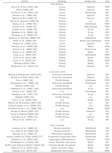
(19) 2.1.4 2.2. 2.3. Multiscale approaches . . . . . . . . . . . . . . . . . . . . . . . . . . 27. Detection criteria . . . . . . . . . . . . . . . . . . . . . . . . . . . . . . . . . 30 2.2.1. Thresholding . . . . . . . . . . . . . . . . . . . . . . . . . . . . . . . 31. 2.2.2. Local peak search. 2.2.3. Multiscale vision model . . . . . . . . . . . . . . . . . . . . . . . . . 35. 2.2.4. Other detection criteria . . . . . . . . . . . . . . . . . . . . . . . . . 37. . . . . . . . . . . . . . . . . . . . . . . . . . . . . 33. Results . . . . . . . . . . . . . . . . . . . . . . . . . . . . . . . . . . . . . . . 40 2.3.1. Evaluation measures . . . . . . . . . . . . . . . . . . . . . . . . . . . 40. 2.3.2. Analysis of the results . . . . . . . . . . . . . . . . . . . . . . . . . . 41. 2.4. Discussion . . . . . . . . . . . . . . . . . . . . . . . . . . . . . . . . . . . . . 45. 2.5. Conclusions . . . . . . . . . . . . . . . . . . . . . . . . . . . . . . . . . . . . 48. 3 Quantitative evaluation of astronomical source detection methods 3.1. 3.2. 3.3. 49. Methods . . . . . . . . . . . . . . . . . . . . . . . . . . . . . . . . . . . . . . 50 3.1.1. SExtractor . . . . . . . . . . . . . . . . . . . . . . . . . . . . . . . . 52. 3.1.2. SAD . . . . . . . . . . . . . . . . . . . . . . . . . . . . . . . . . . . . 52. 3.1.3. Mopex . . . . . . . . . . . . . . . . . . . . . . . . . . . . . . . . . . . 53. 3.1.4. González-Nuevo method . . . . . . . . . . . . . . . . . . . . . . . . . 53. 3.1.5. SourceMiner . . . . . . . . . . . . . . . . . . . . . . . . . . . . . . . 54. 3.1.6. DS . . . . . . . . . . . . . . . . . . . . . . . . . . . . . . . . . . . . . 55. 3.1.7. Astrometry.net . . . . . . . . . . . . . . . . . . . . . . . . . . . . . . 55. 3.1.8. Perret method . . . . . . . . . . . . . . . . . . . . . . . . . . . . . . 56. Quantitative evaluation . . . . . . . . . . . . . . . . . . . . . . . . . . . . . 56 3.2.1. Test datasets . . . . . . . . . . . . . . . . . . . . . . . . . . . . . . . 56. 3.2.2. Reference catalogues . . . . . . . . . . . . . . . . . . . . . . . . . . . 58. 3.2.3. Evaluation measures . . . . . . . . . . . . . . . . . . . . . . . . . . . 61. 3.2.4. Experimental results . . . . . . . . . . . . . . . . . . . . . . . . . . . 64. Discussion . . . . . . . . . . . . . . . . . . . . . . . . . . . . . . . . . . . . . 69 xiv.

(20) 3.4. 3.3.1. Performance of the detection methods . . . . . . . . . . . . . . . . . 69. 3.3.2. Image datasets . . . . . . . . . . . . . . . . . . . . . . . . . . . . . . 72. 3.3.3. Detection strategy . . . . . . . . . . . . . . . . . . . . . . . . . . . . 77. Conclusions . . . . . . . . . . . . . . . . . . . . . . . . . . . . . . . . . . . . 80. 4 Faint source detection in aperture synthesis radio images 4.1. Multiresolution analysis on thresholded images . . . . . . . . . . . . . . . . 84 4.1.1. 4.2. 4.3. 4.4. 83. Algorithm steps . . . . . . . . . . . . . . . . . . . . . . . . . . . . . . 85. Slope stability of a radial contrast function . . . . . . . . . . . . . . . . . . 88 4.2.1. Definition of the radial contrast function . . . . . . . . . . . . . . . . 88. 4.2.2. Algorithm steps . . . . . . . . . . . . . . . . . . . . . . . . . . . . . . 90. Boosting classification system . . . . . . . . . . . . . . . . . . . . . . . . . . 90 4.3.1. Dictionary building process . . . . . . . . . . . . . . . . . . . . . . . 91. 4.3.2. Training and testing processes. 4.3.3. Algorithm steps . . . . . . . . . . . . . . . . . . . . . . . . . . . . . . 93. . . . . . . . . . . . . . . . . . . . . . 92. Test datasets . . . . . . . . . . . . . . . . . . . . . . . . . . . . . . . . . . . 93 4.4.1. Simulated data . . . . . . . . . . . . . . . . . . . . . . . . . . . . . . 95. 4.4.2. GMRT observations . . . . . . . . . . . . . . . . . . . . . . . . . . . 96. 4.4.3. ATCA observations of the Phoenix Deep field . . . . . . . . . . . . . 98. 4.5. Experimental results . . . . . . . . . . . . . . . . . . . . . . . . . . . . . . . 99. 4.6. Discussion . . . . . . . . . . . . . . . . . . . . . . . . . . . . . . . . . . . . . 107. 4.7. Conclusions . . . . . . . . . . . . . . . . . . . . . . . . . . . . . . . . . . . . 114. 5 Multiscale Distilled Sensing: source detection for long wavelength images. 117. 5.1. Distilled Sensing . . . . . . . . . . . . . . . . . . . . . . . . . . . . . . . . . 118. 5.2. DS in multiscale space . . . . . . . . . . . . . . . . . . . . . . . . . . . . . . 120 5.2.1. 5.3. Algorithm steps . . . . . . . . . . . . . . . . . . . . . . . . . . . . . . 121. Experimental results . . . . . . . . . . . . . . . . . . . . . . . . . . . . . . . 122 xv.

(21) 5.4. Discussion . . . . . . . . . . . . . . . . . . . . . . . . . . . . . . . . . . . . . 125. 5.5. Conclusions . . . . . . . . . . . . . . . . . . . . . . . . . . . . . . . . . . . . 133. 6 Conclusions. 135. 6.1. Summary of the thesis . . . . . . . . . . . . . . . . . . . . . . . . . . . . . . 135. 6.2. Contributions . . . . . . . . . . . . . . . . . . . . . . . . . . . . . . . . . . . 137. 6.3. Future work . . . . . . . . . . . . . . . . . . . . . . . . . . . . . . . . . . . . 138. A Parameter setting. 141. A.1 Quantitative evaluation of methods . . . . . . . . . . . . . . . . . . . . . . . 141 A.2 Faint source detection methods . . . . . . . . . . . . . . . . . . . . . . . . . 143 A.3 Multiscale Distilled Sensing . . . . . . . . . . . . . . . . . . . . . . . . . . . 145 Bibliography. 147. xvi.

(22) Resum Aquesta tesi se centra en la detecció automàtica de fonts (objectes) en imatges astronòmiques. L’ús d’eines automàtiques per a realitzar aquest tipus de tasca esdevé d’una gran importància en l’àmbit astronòmic degut a la creixent quantitat de dades i a la ineficiència i imprecisió de les inspeccions manuals. En primer lloc, s’analitza de forma exhaustiva l’estat de l’art d’aquest tema, presentant una nova classificació de tècniques i destacant els seus principals punts forts i febles. Complementàriament, també es proporciona una avaluació quantitativa d’alguns dels mètodes més destacats. En segon lloc, es presenten tres propostes diferents per a la detecció de fonts febles en imatges de radiointerferometria (sı́ntesi d’obertura): la primera, anomenada WALT, combina la transformada wavelet amb una binarització local; la segona, anomenada RCF, es basa en el comportament estructural d’una funció de contrast radial; i la tercera, realitza una classificació supervisada de pı́xels per mitjà de caracterı́stiques locals i d’un mètode de boosting. Finalment, també es presenta una nova proposta per tractar amb imatges infraroges i de radiofreqüència. Aquest mètode, anomenat multiscale distilled sensing (MDS), es basa en l’ús combinat de la transformada wavelet i un mètode molt innovador anomenat distilled sensing. Els resultats experimentals i l’avaluació duta a terme amb imatges sintètiques i reals han demostrat que el rendiment de les quatre propostes és millor que el d’altres mètodes de l’estat de l’art, tant pel que fa a fiabilitat com a completesa.. xvii.

(23) xviii.

(24) Resumen Esta tesis se centra en la detección automática de fuentes (objetos) en imágenes astronómicas. El uso de herramientas automáticas para realizar este tipo de tarea es sumamente importante en el ámbito astronómico debido a la creciente cantidad de datos e a la ineficiencia e imprecisión de las inspecciones manuales. En primer lugar, se analiza de forma exhaustiva el estado del arte de este tema, presentando una nueva clasificación de técnicas y destacando sus puntos fuertes y débiles. Complementariamente, también se proporciona una avaluación cuantitativa de algunos de los métodos más destacados. En segundo lugar, se presentan tres propuestas diferentes para la detección de fuentes débiles en imágenes de radiointerferometrı́a (sı́ntesis de apertura): la primera, llamada WALT, combina la transformada wavelet con una binarización local; la segunda, llamada RCF, se basa en el comportamiento estructural de una función de contraste radial; y la tercera, realiza una clasificación supervisada de pı́xeles mediante caracterı́sticas locales y un método de boosting. Finalmente, también se presenta una nueva propuesta para tratar con imágenes infrarrojas y de radiofrecuencia. Este método, llamado multiscale distilled sensing (MDS), se basa en el uso combinado de la transformada wavelet y un método muy innovador llamado distilled sensing. Los resultados experimentales y la avaluación llevada a cabo con imágenes sintéticas y reales han demostrado que el rendimiento de las cuatro propuestas es mejor que el de otros métodos del estado del arte, tanto en cuanto a fiabilidad como a completitud.. xix.

(25) xx.

(26) Abstract This thesis is focused on the automatic detection of sources (objects) in astronomical images. The use of automatic algorithms to perform such a task becomes of great importance in the astronomical field because of the increasing amount of data and the inefficiency and inaccuracy of manual inspection. In the first place, we exhaustively analyze the state of the art on this topic, presenting a new classification of techniques and pointing out their main strengths and weaknesses. A complementary quantitative evaluation of some of the most remarkable methods in the literature is also provided. Afterwards, we present three different proposals to detect faint sources in radio aperture synthesis images: the first, a method that combines the multiscale wavelet transform and local thresholding (WALT); the second, a method based on the structural behaviour of an intensity radial contrast function (RCF); and the third, a supervised method that classifies pixels by means of local features (filtered patches) and a boosting classifier. Finally, we also present a new proposal to deal with infrared and radio images. This method, called multiscale distilled sensing (MDS), is based on the combined use of the wavelet transform and an innovative method called distilled sensing. The experimental results and the evaluation performed with synthetic and real data points out that the performances of our four proposals are better than state-of-the-art approaches in terms of both reliability and completeness of the detections provided.. xxi.

(27) xxii.

(28) Chapter. 1. Introduction. The universe contains billions of astronomical objects in constant evolution. With the desire of better understanding the cosmos, astronomers obtain thousands of images of these objects. These astronomical images provide information about the great variety of celestial objects (sources) existing in the universe, the physical processes taking place in them, and the formation and evolution of the cosmos. Over the last few years highresolution mappings and catalogues of astronomical objects have been published by many observatories that use vanguard technology located both on the Earth’s surface and in orbit [1, 19, 95, 68, 4]. These telescopes work not only in the optical domain, but in the whole range of the electromagnetic spectrum. Therefore, it is a common practice to acquire images with instruments that capture photons of frequencies not perceptible to human eyes like radio frequencies or X-rays [10]. Observing the same section of sky at different frequencies produces different types of images. Combined and comparative analyses of these images provide more comprehensive information about the objects in this area. However, detecting objects in astronomical images is not an easy task even for experienced astronomers. They are at distances measured in light-years, so it is very likely that they will appear as faint bright points or blended with other objects. Also, it is possible that some spots in these images may be considered as objects when actually they are not. For all these reasons, astronomical images need an exhaustive analysis in order to detect precisely when an object is present and when not. The optimal way to carry out these analyses would be with astronomical experts searching for the various objects to be found in these images. However, due to the large amount of data and the fact that many objects can be almost imperceptible, a search by humans is inefficient, very slow, and inaccurate, if not almost impossible. Hence, it is necessary to develop highly robust, fast, efficient, and computer automated algorithms to detect the astronomical objects by means of image processing and computer 1.

(29) 2. Chapter 1. Introduction. vision techniques. The automatic detection of sources in astronomical images seems to be quite a straightforward task compared to other computer vision problems: the typical scenario is dealing with light-emitting sources on dark backgrounds. Nevertheless, there are some difficulties associated with astronomical images that make this a complicated task. On the one hand, many astronomical objects do not show clear boundaries since their intensities are similar to the detection levels (i.e. those close to the background level) and they are mixed with noise components. On the other hand, especially in the case of wide-field deep images showing multiple sources, the sizes and intensities of the different objects present may vary considerably. Therefore, the images can have a high dynamic range (i.e. ratio between the highest and lowest intensity level) and a large spatial dynamic range (i.e. ratio between the largest and smallest detectable structure). These facts may cause image display problems due to the limited range of intensities perceptible by human vision. Therefore, the main challenge of object detection in astronomical images is to separate those pixels that belong to astronomical bodies from those that belong to the background or noise to be able to specify the coordinates where these bodies are located afterwards. Since this goal may require searching through connected regions of pixels constituting objects, this task is also referred to as object segmentation in the computer vision community [82]. Nevertheless, in this document we will often refer to the localization of the central coordinates of the sources as detection. The final outcome of this detection process is a list of the objects’ coordinates found (also known as the catalogue). The use of automatic tools to perform this task becomes of great importance in the astronomical field because of the increasing amount of data (usually many large-sized images per survey or observation with up to thousands of sources) and the inefficiency and inaccuracy of manual inspection.. 1.1. Astronomical images. Despite the fact that all astronomical images are greyscale images with a high dynamic range, there are several types of images used for different purposes and with different characteristics.. 1.1.1. Types of astronomical images. People are able to perceive visible light through their eyes. This light is within the electromagnetic spectrum through which the Sun emits most of its radiated energy. In fact,.

(30) 1.1. Astronomical images. 3. Figure 1.1: Electromagnetic spectrum.. visible light is only a small portion of all the electromagnetic radiation that travels through space. Initially, the study of the universe was focused mainly on the visible band, with the building of observatories that included optical telescopes with associated devices like spectrometers or photometers. However, due to the large amounts of relevant information in the invisible bands, astronomers also made efforts to develop an astronomy able to capture non-visible radiation emitted at different frequencies (and therefore, different wavelengths) as can be seen in the electromagnetic spectrum in Figure 1.1. On the one hand, there is radiation emitted at frequencies lower than the visible range (with wavelengths between 400 and 700 nm), such as radio and infrared. On the other hand, there is the radiation emitted at frequencies higher than the visible range, such as ultraviolet, X-rays, and γ-rays. Various celestial bodies, gas, dust, and other elements may be visible at specific frequencies, and therefore, different types of images are used depending on the elements to visualize. Moreover, a common practice in astronomy is to superimpose images at different frequencies in order to combine the information provided at each band and are therefore called multiband images. An analysis of the sky at different frequencies allows the study of the phenomena of the universe, from the least energetic to the most, from the coolest to the hottest radiation. Most non-visible bands, except for radio and the zones of infrared and ultraviolet near visible light, are blocked by the atmosphere, and for this reason, astronomy in these bands could not be developed until the advent of the space age in the sixties and seventies. Until this time, optical astronomy allowed astronomers to observe stars and other phenomena which emit at medium temperatures such as the sun. A couple of examples of optical.

(31) 4. Chapter 1. Introduction. Figure 1.2: Two examples of telescopes. On the left, the Hubble Space Telescope in orbit. On the right, the ALMA interferometer.. telescopes are the Hubble Space Telescope [69] (shown in orbit in Figure 1.2, left) and the W. M. Keck Observatory [106] (in Hawaii). Nevertheless, astronomy at radio frequencies was developed in the thirties, before than at any other frequency, since it was directly linked to the development of the radio receiver. Radio astronomy is carried out by means of directional radio antennas and, unlike optical images, radio images have poor resolution (the ability to see in detail given by the ratio of the wavelength and the instrument diameter). The astronomers calculated that to achieve the same resolution in radio as with optical, they would need instruments 100,000 times greater (a non-viable size, since it is technologically impossible to build antennas over 100 meters). To solve this problem, they decided to form images by correlating (by pairs) the signal reached by multiple antennas located in fields, laid out in very large arrays (along kilometres). These antennas point to the same stellar object, but, as they are spaced out, the light reaches them at different moments albeit tiny, simulating a huge antenna with a diameter of kilometres. Afterwards, the different signals are correlated and, with some mathematical operations, a high resolution image is formed. The whole set of antennas is called a radio interferometer. Some examples of interferometers are the Very Large Array [95], the Very Long Baseline Array [68], the Atacama Large Millimeter/submillimeter Array (ALMA) [112] (shown in Figure 1.2, right) and the Square Kilometre Array (SKA) [18] (in development). Astronomers can observe the so-called near-infrared (infrared radiation close to the visible part of the spectrum) with the same devices used in optical. The same happens with near-ultraviolet radiation. As infrared radiation moves away from visible light, the telescope must be placed at a higher altitude, even above the atmosphere. Infrared observations are used to observe emissions of cold clouds of gas and dust. Some examples.

(32) 1.1. Astronomical images. 5. of infrared telescopes in space are the Herschel Space Observatory [79], the Spitzer Space Telescope [108], and the Wide-field Infrared Survey Explorer (WISE) [19], even though the Hubble Space Telescope can observe at near-infrared frequencies as well. Some others have been placed in aeroplanes, such as the Stratospheric Observatory for Infrared Astronomy (SOFIA) [24] or on the Earth’s surface, such as the James Clerk Maxwell Telescope at the Keck Observatory. To achieve better resolution, there are even infrared interferometers, such as the one at the Keck Observatory. Observations at high frequencies are usually performed from the upper atmosphere or from space using rockets and satellites. In ultraviolet, it is possible to visualize massive young stars and very old ones, which are very hot, and therefore, emit in an area of the spectrum close to blue and ultraviolet. Some examples of space telescopes that observe at ultraviolet frequencies are the Hubble Space Telescope (HST) and the Galaxy Evolution Explorer (GALEX) [60]. With X-rays, the energies are very high and show violent phenomena or sources with extremely hot gases. In γ-rays, very violent phenomena such as black holes, supernova explosions, or the destruction of atoms are especially detected. Some of the X-ray satellites in use today include the X-ray Multi-Mirror Mission-Newton (XMM-Newton) [45] and the Chandra X-ray Observatory [107], whereas some of the γ-ray satellites currently in orbit are the INTErnational Gamma-Ray Astrophysics Laboratory (INTEGRAL) [111], the Astro-Rivelatore Gamma a Immagini Leggero (AGILE) [66] and the Fermi Gamma-ray Space Telescope [4].. 1.1.2. Celestial coordinate system. A common practice in astronomy is to measure the position of objects by means of a celestial coordinate system. They are usually spherical systems, although they also have a rectangular implementation. The most commonly used is the equatorial coordinate system which consists of projecting the latitudes and longitudes of the Earth onto the celestial sphere (an imaginary sphere concentric with Earth with a radius that can be considered as infinite). Equatorial coordinates are expressed as a pair: the latitudinal direction is called declination (Dec - measured in degrees from -90◦ to 90◦ ) and the longitudinal direction is called right ascension (RA - measured in degrees from 0◦ to 360◦ or in hours from 0 to 24). Other alternative celestial coordinate systems are used as well. The galactic coordinate system uses the Sun as the origin and the galactic plane (coincident with the plane of the Milky Way galaxy) as its fundamental plane. The galactic latitude (b - measured.

(33) 6. Chapter 1. Introduction. in degrees from -90◦ to 90◦ ) is the angular distance above or below the galactic plane, whereas the galactic longitude (l - measured in degrees from 0◦ to 360◦ ) is the angular distance along the galactic plane. On the other hand, the ecliptic coordinate system uses the Earth as its origin and the ecliptic (the plane that includes the orbits of the Earth and the Sun) as its fundamental plane. The ecliptic latitude (measured in degrees from -90◦ to +90◦ ) is the angular distance above or below the ecliptic, whereas the ecliptic longitude (measured in degrees from 0 to 360) is the angular distance along the ecliptic.. 1.1.3. The FITS format. FITS is the acronym for Flexible Image Transport System [75] and is the standard computer data format widely used by astronomers to store, transmit and manipulate data files. Unlike many image formats, FITS is designed specifically for scientific data, and for this reason, it offers the possibility of attaching additional data as photometric and spatial calibration information. It is basically designed to store scientific datasets consisting of multidimensional arrays and 2-dimensional tables containing rows and columns of data. FITS is also often used to store non-image data, such as electromagnetic spectra, photon lists, data cubes, or even structured data. FITS files allow extensions containing data objects. For instance, one file may store different exposures of the same area of the sky such as X-rays and infrared exposures. FITS was originally developed in the late seventies to provide a way to exchange astronomical data between computers of different types, with different word lengths, and different means to express numerical values. It was in 1981 when the first version of the FITS format became standardized, and after successive updates, the last version released was the 3.0, approved in July 2008. The most commonly used type of FITS data is a data array of arbitrary dimension (for example, the image) and one or more headers. The file consists of several structures called HDU (header and data units) including a header and the data described by the header. The primary HDU contains an n-dimensional array of pixels (e.g. a 1-D spectrum, a 2-D image, or a 3-D data cube). Additional HDUs may appear after the primary one, and are called FITS extensions. Three types of extensions are available: image extensions, which are n-dimensional arrays of pixels, like in a primary array; ASCII table extensions, which are rows and columns of data in the ASCCI character format; and binary table extensions, which are rows and columns of data in a binary representation. An interesting point is that the information is stored in headers in a humanly readable.

(34) 1.2. Astronomical sources. 7. way, so that users can examine the headers and understand the file’s content such as the size, date and time, origin, coordinates, binary data format, free-form comments, history of the data, and anything else. For more detail, see the FITS standard [75].. 1.2. Astronomical sources. An astronomical source is the origin of something that suggests the presence of an astronomical object. Hereafter we are going to use the terms source and object without distinction as those stellar bodies that can be detected in images. Behind the sources detected we can find a variety of different astronomical bodies. For instance, in our own Solar System we find a star (the Sun), eight planets, at least five dwarf planets (objects massive enough to be nearly spherical and which have not cleared a path around a star), hundreds of natural satellites, thousands of comets and millions of asteroids, among others. Beyond the Solar System, apart from the objects already mentioned, we find an incalculable number of other sources such as stars and galaxies as well as gas, dust and cosmic rays. Stars are basically composed of hydrogen and helium and are formed when a region achieves enough density of matter (gas and dust) due to a gravitational instability. Thus, a compact sphere with enough gravity at its center is formed. Afterwards, it starts to fuse hydrogen in its core producing large amounts of energy. Once the hydrogen in the core is exhausted (after up to billions of years), the evolution of the star depends on its mass, so that it can become a white dwarf (a stable cool star) or a red giant (a stable star that fuses hydrogen in a shell outside the core), or it can even explode: massive and binary stars may explode in a violent phenomenon called supernova, while white dwarfs may explode in a less energetic phenomenon called nova. A supernova remnant can form new astronomical bodies including new stars. Groups of stars and stellar remnants, gas and dust gravitationally bound and evolving together in the Universe are known as galaxies. Depending on their morphology, they can be classified as elliptical, spiral or irregular. Interactions between galaxies are relatively frequent. For example, they may collide, which happens when one passes through the other. This collision may produce changes in the morphology of the galaxies. The interaction of gas and dust between the two galaxies produces disruptions and compressions and favours the appearance of zones of star formation. Some examples of stars and galaxies are shown in Figure 1.3..

(35) 8. Chapter 1. Introduction. Figure 1.3: Some examples of astronomical objects. On the left, several isolated stars, in the middle, a cluster of stars, and on the right, an elliptical galaxy. All these images have been extracted from the Hubble website [69].. 1.2.1. Source morphology. Sources may present different shapes depending on the type of astronomical object they actually are. When the angular size of an object is smaller than the angular resolution of the telescope used to perform the observation, the object appears in images as a point source (also called unresolved). The response of a telescope to a point source is called the point spread function (PSF, although sometimes it is also known as the beam) [10]. It describes the two-dimensional distribution of light in the telescope’s focal plane, and therefore, the representation of a point source in an image is the convolution of the object with the PSF, as shown in Figure 1.4. Hence, the size of a point source is given by the PSF of the acquisition instrument, and is usually measured through its full width at half maximum (FWHM). Great efforts are taken in order to reduce the size of the PSF in telescopes so that the signal is not spread out over too many pixels. Point sources typically have only a few pixels, and because of this, are sometimes confused with image noise. On the other hand, sources that exceed the size of the PSF are commonly known as extended or resolved. They might still have compact spherical shapes (e.g. some distant galaxies) or be more irregular (e.g. supernova remnants). An example of an astronomical image with sources of different morphology is shown in Figure 1.5. Notice that saturating the image by changing the contrast, the structure of some extended sources is lost, but many faint sources appear..

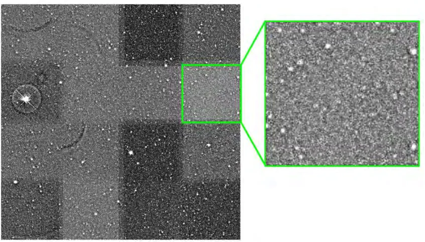
(36) 1.2. Astronomical sources. 9. Figure 1.4: Graphical representation of the effect of the PSF in images.. Figure 1.5: Radio image with different contrast stretching (0.1% of outliers eliminated on the left, and 2% on the right). These images contain extended sources encircled in green, irregular sources such as that at the top of the image, and multiple point sources..

(37) 10. 1.3. Chapter 1. Introduction. Background and noise. In astronomical images, empty parts of the sky are known as the background. Hereafter, we talk about the background and the sky without distinction. Even if an object is not present in these regions of the sky, a low luminosity mostly due to the light emitted by nearby sources, is always present. Images taken through the atmosphere may be polluted by light from man-made sources such as cities. Some regions of the background may be considered as such by human eyes, however, they may hide sources visible in other frequency bands or those so faint that they are detectable only by computer tools. Furthermore, the background is diffuse, meaning that it is difficult to specify the exact line that indicates where the sources end and where the background begins. Moreover, the background is normally non-homogeneous due to the fact that some astronomical images need a long exposure time. Also, there are changes in the atmospheric conditions so sometimes they are mosaics made up of different images pointing at different coordinates at different moments, as can be seen in Figure 1.6. Astronomical images are characterized by the presence of noise. It is one of the main disadvantages in astronomical detection, since it makes the detection process difficult. There are different types of noise according to their origin, such as shot, thermal and readout. Shot noise is due to the random variations in the number of light photons acquired by the instruments; thermal noise is due to the intrinsic thermal fluctuations in the acquisition devices that knock some electrons free; and the readout noise is due to the imperfect conversion from an analogue signal to a digital value in an electronic device [43]. Noise in images is usually taken as additive Gaussian and/or Poisson. For instance, in CCD (Charge-Coupled Device) images, the arrival of photons may generate Poisson noise while readout noise is commonly Gaussian. However, to simplify, in longer wavelength bands (basically optical, infrared and radio), the noise and the background are assumed to follow a Gaussian distribution. On the other hand, shorter wavelength bands present mainly Poisson noise since they are acquired by means of photon counters [91]. The amount of noise can be measured through the so-called signal-to-noise ratio (SNR), which is a measure used in many fields to quantify how much a signal has been corrupted by noise. It is calculated by dividing the amount of signal by the amount of noise (see the next chapter for more information), and therefore, the higher the ratio, the lesser the noise impact. Noise can sometimes be estimated through knowledge of the instrument’s properties..

(38) 1.3. Background and noise. 11. Figure 1.6: An infrared mosaic with background variations. This image, courtesy of Dr. J. Martı́ (private communication), is quite noisy and even presents some interferences (the darker curved regions at the top left of the image)..

(39) 12. 1.4. Chapter 1. Introduction. Astronomical imaging pipeline. In an astronomical imaging pipeline, also known as data reduction, several steps are carried out in order to generate the catalogues with features of the objects present in a region of the sky. An astronomical catalogue is a list of known astronomical objects that share a common type, morphology, origin or detection method. Astronomical catalogues are usually the outcome of a general map or image of a region of the sky (this is also known as an astronomical survey).. 1.4.1. Acquisition process. Astronomical observations are made in observatories by means of large telescopes. The most widely-used telescopes are optical, able to observe the visible light emitted by stellar bodies and some wavelengths of ultraviolet and infrared bands. These telescopes are generally composed of two or three reflector mirrors or lenses to gather and focus light photons. Sometimes, some filters are used in the telescope to select specific zones of the electromagnetic spectrum (a set of these filters covering an important part of the spectrum is known as a photometric system). They are usually placed in large observatories in high places like mountaintops to take advantage of optimal climatic conditions such as clear skies or dry environments due to thermal inversion as dampness is below the observatories’ location. As the atmosphere may distort the observations (the blurring and twinkling of objects caused by turbulences in the atmosphere is called seeing), sometimes these telescopes and some at other wavelengths, are placed at higher altitudes using aeroplanes and satellites. Following similar principles, there are other types of telescopes according to the band they observe. Most of them, such as infrared, ultraviolet, X-ray, and γ-ray telescopes, are found above the atmosphere. In order to form a radiation image that reaches the telescope, a CCD camera is frequently used. They are used mainly due to their high sensitivity to most of the electromagnetic spectrum, especially the visible range, their linear response to the light, their reduced size, and their low cost. CCD cameras have an array of CCD sensors, each of which corresponds to a pixel in the image. These sensors are based on the photoelectric effect, which converts its received light into electric current to be translated to a pixel intensity in the digital image afterwards. CCD cameras are able to capture visible, ultraviolet, infrared (although in this band, infrared detector arrays are used as well) and even X-ray bands. On the other hand, as we have already mentioned, radio frequencies are captured.

(40) 1.4. Astronomical imaging pipeline. 13. through directional radio antennas. To have high resolution in radio, interferometry must be used, which reaches radio emissions with large arrays of antennas. Moreover, to preserve an angular resolution (antennas have a concave shape), a technique called aperture synthesis is used. This technique simulates the distribution of the set of antennas by mathematical corrections, taking into account the shape the huge simulated antenna should have (a parabola or a dish shape). In radio, the image is formed by the interpretation of the signal reached by the interferometer. In γ-rays (and sometimes also in X-rays), the image is generally created by photon counters.. 1.4.2. Preprocessing. Several preprocessing steps are used to remove instrumental signatures from the data. For instance, a typical practice in CCD imaging is to calibrate the data by means of bias and dark current subtraction and flat fielding. Bias frames are images taken with no light (shutter closed) and with an exposure time of zero used to measure the signal of the CCD pixels; dark frames are images taken with no light in a given exposure time used to measure the dark current due to the thermal emission of the CCD pixels; and the flat fields are images taken when a homogeneous source of light is exposed and are used to measure the light sensitivity of the CCD pixels [43]. Some pixels in the image may be missing or corrupt (they are also known as bad or dead pixels) due to defects in the CCD or to cosmic rays (high energy particles). Some techniques used to deal with these outliers are, for instance, simple filtering, image reconstruction (such as replacements or interpolations) or inpainting. Additionally, to attenuate background variations such as noise or interferences, several instances of the same observation can be taken and pixel means or medians can be performed [114, 32, 115, 88]. In radio interferometric images, where strong fringe patters are usually present, image restoration through deconvolution is commonly used. The so-called CLEAN algorithm [39] is the most widely used algorithm in these images. It iteratively searches peaks (sources) in the image, subtracts the gain of the beam at these peaks and convolves them with an idealized beam (usually a Gaussian).. 1.4.3. Source extraction. Source detection can be considered as the first step of source extraction and consists of extracting properties and characteristics of the objects present in an astronomical image..

(41) 14. Chapter 1. Introduction. Once the sources are located, a common practice is to measure their intensity radiation (also known as flux). This process is called photometry and can provide information about the structure of the object, its temperature, distance or age. Photometry techniques aim to measure the light emitted by the source and discard the light from the sky. Two different types of photometry are commonly used: aperture and differential. In aperture photometry, the level of the sky is measured by averaging the intensity pixels of an annulus around the source center that do not include the source, and afterwards, this value is subtracted from the addition of the intensity of the pixels within a circle surrounding the source (aperture). On the other hand, differential photometry measures the brightness of the sources relative to reference sources with constant brightness. It is typically used to determine the evolution of variable stars. In astronomy, the brightness can be measured in different ways. The amount of energy transferred to CCD pixels or photon counters is mostly measured in terms of flux in Jansky (Jy) units. However, the logarithmic measure of the brightness of the objects relative to stars of known brightness is widely used as well. It is so-called magnitude and can be calculated as follows:. m = mref − 2.5 log10 (. f lux ), f luxref. (1.1). where mref is the photometric zero point: the magnitude of a star with a brightness considered as reference (the star Vega has been classically assumed to have zero magnitude). f luxref corresponds to the flux of the reference star. Note that the smaller the magnitude, the brighter the source. Additionally, flux in radio astronomy is sometimes measured in terms of brightness temperature (the temperature of a black body in thermal equilibrium) in K units. The determination of the position of objects in terms of celestial coordinates is then carried out. This process is called astrometry and commonly uses the coordinates of sources in the image well-located in other catalogues to determine the position of objects in the image with unknown coordinates. Additionally, as many observations are performed pointing to well-known coordinates, this prior information can also be used to determine the astrometry in images. Some source extraction methods also incorporate a source classification step to figure out the type of astronomical bodies behind the sources. For instance, some software applies star/galaxy classification or galaxy morphology determination steps..

(42) 1.5. Research framework. 1.5. 15. Research framework. This thesis is located within the framework of two research projects in which the Computer Vision and Robotics (VICOROB) group [103] of the University of Girona [100] has been recently involved: “Observational and theoretical studies of high energy galactic sources from the radio to the VHE γ-rays” (reference AYA2007-68034-C03-03) awarded by the Ministerio de Educación y Ciencia (2008-2010), for which Dr. Marta Peracaula was responsible; and “High-energy phenomena in stellar objects. Theory and multiwavelength observations” (reference AYA2010-21782-C03-02) awarded by Ministerio de Ciencia e Innovación (2011-2013), for which Dr. Jordi Freixenet was responsible. Both projects were coordinated by the teams of the Department of Astronomy and Meteorology [97] and the Institute of Sciences of the Cosmos [98] of the University of Barcelona [99], led by Dr. Josep Maria Paredes. The third member involved in the projects was the team of the Department of Physics of the University of Jaén [101], led by Dr. Josep Martı́. The main role of VICOROB in these projects was closely related to that of this thesis. It specifically consists of performing research on astronomical source detection algorithms in images of different natures, paying special attention to the development of detection and segmentation algorithms for radio images.. 1.6. Objectives. As part of the two projects just mentioned, the main goal of this thesis is the analysis and development of automatic algorithms to detect sources in astronomical images. This goal refers to the building of catalogues containing the coordinates, in terms of pixels, of the centroid of sources present in images. This general objective can be divided into three specific parts pertaining to the different stages of this thesis: 1. An exhaustive analysis of the state of the art in astronomical source detection. This includes a review of the main methods used over the last few years as well as the proposal of a new classification of methods according to their main steps. This second task arises from the lack of an updated review of astronomical.

(43) 16. Chapter 1. Introduction. detection techniques at the beginning of this thesis. 2. A quantitative analysis of some of the most promising methods found in the state of the art. This evaluation includes some of the most widely used detection algorithms as well as other innovative methods that have recently emerged. Included is the selection of an appropriate common dataset to level the playing field consisting of optical, infrared and radio images. Accurate catalogues of sources are also needed in order to evaluate the detection performance of the methods. 3. The development of several proposals to automatically detect sources in different types of astronomical images. Our main aim is the implementation of different methods able to deal with different types of images at different bands. However, as the research projects linked to this thesis are mainly focused on radio frequency images, more importance is given to the use of radio images. The results obtained with these proposals in different datasets will also be compared to those obtained with widely-used state-of-the-art methods.. 1.7. Document structure. This thesis is structured as follows: • Chapter 1. Introduction. This current chapter has explained the main points this thesis deals with, such as what is and what the automatic detection of sources in astronomical images involves. The planning and goals of this thesis have been presented as well. The following chapters explain, in detail, the current techniques in this field and introduce new proposals. • Chapter 2. Review of source detection in astronomical images. After Chapter 1, a wide variety of astronomical detection techniques that have appeared over the last few years is analyzed, pointing out their main advantages and drawbacks in a qualitative way. We introduce a new classification based on the image transformations and the detection criteria the methods use. Finally, the performance of the methods is discussed according to their reported results. • Chapter 3. Quantitative evaluation of source detection methods. After reviewing the different techniques used to detect sources in Chapter 2, we present a quantitative evaluation of some of the most salient methods found in the literature. They are tested with a unified dataset consisting of optical, infrared, and.

(44) 1.7. Document structure. 17. radio frequency images. Respective catalogues of the images are used to evaluate the performance of these methods in terms of reliability of the detections obtained and the number of true sources in the catalogue correctly identified. An extended discussion is presented regarding the methods, the strategies they use and the type of images. • Chapter 4. Faint source detection in aperture synthesis radio images. After the exhaustive evaluation of strategies in Chapters 2 and 3, three new approaches to detect faint sources based on different techniques are presented. They come out of what we considered as being some of the most interesting techniques in the state of the art: the first combines multiscale decomposition and local thresholding; the second performs a radial contrast analysis of neighbourhoods of pixels; whereas the third classifies pixels by means of local features and a boosting classifier. After testing them on radio interferometric datasets, their results are compared to those achieved with algorithms widely-used by the astronomical community. • Chapter 5. Multiscale source detection for long wavelength images. Another proposal to deal with the detection of sources in radio and infrared images is presented in this chapter. It is based on the combination of commonly used multiscale transforms and the promising Distilled Sensing method. The combination of these methods allows a better performance than using only Distilled Sensing. The new proposal has been applied to different long wavelength datasets and the results obtained have been compared to commonly-used detection software. • Chapter 6. Conclusions. This final chapter sums up the main conclusions extracted from this work. Based on these, possible solutions and future work are set out..

(45) 18. Chapter 1. Introduction.

(46) Chapter. 2. Review of source detection in astronomical images. Astronomical detection is usually the first step in the process of building astronomical catalogues. For this reason, after astronomical detection, two other processes are also performed: classification, which categorizes the objects into different types (e.g. stars, clusters, galaxies, extended objects, etc.), and photometry, to account for the flux, magnitude or intensity of the objects. The whole process of building a catalogue is also known as source extraction. The development of automated algorithms to detect astronomical objects has become a research topic of interest for the astronomical community. Even thought these algorithms perform the same actions that an experienced astronomer can do with an appropriate display system, their importance relies on the fact that algorithms can do these things quickly, repeatedly, and always with maximum objectivity (properties a person can not guarantee). As stated by Goderya and Lolling [25], their importance becomes apparent in wide fields or large surveys with thousands of sources that can have intensities at detection levels. In these cases, a human search is inefficient, very slow, and inaccurate, if not almost impossible. The first automated methods for astronomical object detection had already been developed in the seventies, and have evolved until today, although at a relatively slow pace because simple image processing techniques are already used to achieve better results than those performed manually by experts. Nevertheless, more accurate and reliable detection techniques are increasingly required by astronomers so more complex strategies have been implemented. We are aware that astronomical imaging is a broad subject and images acquired at. 19.

(47) 20. Chapter 2. Review of source detection in astronomical images. different frequency bands present different features and behaviours. However, we want to give an overview of the most used techniques to find astronomical sources regardless of the origin of the images employed. This does not mean that we obviate the importance of the type of image. By doing this general review we can see whether a given technique performs well with different types of images or if it is more suitable for a specific frequency band. In this chapter we review the current state of the art in astronomical source detection [61], including a detailed analysis of these works, their classification according to the methods used, the image type, and the evaluation of their results. We propose a new classification based on two main steps: image transformation and detection criterion. The first consists of applying changes to the astronomical images to prepare them for further processing, whereas the second consists of classifying pixels that belong to sources and separating them from background pixels, or in finding those pixels where the sources are centred. Moreover, we also analyze the parameters of the strategies reviewed such as the type of image, the reference catalogue, the evaluation measures used and their performance. To the best of our knowledge, this is the first attempt to provide a quantitative and qualitative comparison of detection approaches according to their reported results in the literature.. 2.1. Image transformation. Image transformation is a basic step used to prepare data to achieve a better performance in later steps. Before putting into practice some of the image processing steps, some operations may be applied to suppress undesired distortions or enhance some features for further processing. Image transformation steps transform raw images in some way, creating new images with the same information content as the originals, but with better conditions. Thus, the images are adapted to facilitate later analysis, and to obtain better results. In astronomical imaging, the objectives of image transformation are, for instance, to filter noise, to estimate the background or to highlight the objects. Within this image transformation group, we find techniques such as filtering, deconvolution, transforms, or morphological operations. We present a formal and more accurate classification by dividing the image transformation steps into multiscale strategies, basic image transformations, Bayesian approaches, and matched-filter-based strategies. More information is given in Table 2.1, which presents the different works reviewed according to.

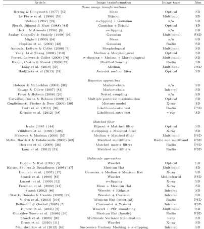
(48) 2.1. Image transformation. 21. the image transformation method, the type of image and the specified detection aim. The methods are grouped by their image transformation strategy. Notice that the different strategy aims may not be exclusive, but are simply the way authors referred to them.. 2.1.1. Basic image transformation. We begin this image transformation review with a range of techniques that, although simple, offer good performance, and hence are widely used throughout the computer vision field. They are basically used to filter noise and estimate background level. Simple filtering techniques such as median or average are used by many authors. They consist of a sliding window centred on a pixel that computes one of the statistics mentioned for all the pixels in the window, and, finally, replaces the central pixel with the computed value. For instance, the median filter was used by Damiani et al. [17] and Makovoz & Marleau [57] to estimate the background level and minimize the effect of bright point source light, while Yang et al. [113], Perret et al. [76], and Lang et al. [50] used it to filter noise and smooth the image. With these two aims, Herzog & Illingworth [37], Mighell [64] and Freeman et al. [21] used the mean filter. Notice that in some cases, pixels in the window with high values are removed to avoid biased values. Background estimation is a common step in astronomical object detection. A good way to carry it out is by using the one used in well-known extraction packages such as Daophot [92] and SExtractor [6]. Their local background estimation is performed by iteratively applying a thresholding based on the mean and standard deviation to eliminate outliers. Afterwards, a value of the true background is calculated as a function of these statistics (Stetson suggested 3×median - 2×mean, while Bertin suggested 2.5×median 1.5×mean). Some authors refer to this background estimation as σ-clipping. Others, such as Vikhlinin et al. [105], Lazzati et al. [52], Perret et al. [76] and Men’shchikov et al. [63] (in multiscale planes) also used this method to deal with the background estimation. Some authors (Irwin [44], Le Fèvre et al. [53] and Slezak et al. [84]) mentioned that they use a method that Bijaoui [7] presented more than thirty years ago. It was based on a Bayesian estimation of the intensity at each point using the histogram of the densities. A model of this histogram was then built, taking into account the granulation and the signal distribution, and obtaining the best threshold to separate the sky from the foreground. Although at first it was a widely used background estimation strategy, it became less common due to its high computational cost..

(49) 22. Chapter 2. Review of source detection in astronomical images. Table 2.1: Summary of the methods’ image transformation. Detection aims stand for: extended source detection (ESD), faint source detection (FSD), point source detection (PSD), and source detection (SD). The term ’n/a’ stands for not available. Article. Image transformation. Image type. Aim. Basic image transformations Herzog & Illingworth (1977) [37]. Mean. Optical. SD. Le Fèvre et al. (1986) [53]. Bijaoui. Multiband. SD. Stetson (1987) [92]. σ-clipping + Gaussian. n/a. SD. Slezak, Bijaoui & Mars (1988) [84]. Gaussian + Bijaoui. Optical. SD. Bertin & Arnouts (1996) [6]. σ-clipping. n/a. SD. Szalay, Connolly & Szokoly (1999) [93]. Gaussian. Multiband. FSD. Mighell (1999) [64]. Mean. n/a. SD. Hopkins et al. (2002) [42]. Gaussian. Radio. SD. Aptoula, Lefèvre & Collet (2006) [3]. Morphological. Multiband. SD. Yang, Li & Zhang (2008) [113]. Median + Morphological. Optical. SD. Perret, Lefèvre & Collet (2008) [76]. σ-clipping + Median + Morphological. Multiband. SD. Haupt, Castro & Nowak (2009)[35]. Distilled Sensing. Radio. SD. Lang et al. (2010) [50]. Median. Multiband. PSD. Hadjiyska et al (2013) [31]. Asterisk median filter. Optical. SD. Bayesian approaches Hobson & McLachlan (2003) [38]. Markov-chain. n/a. SD. Savage & Oliver (2007) [81]. Markov-chain. Infrared. SD. Feroz & Hobson (2008) [20]. Nested sampling. n/a. SD. Carvalho, Rocha & Hobson (2009) [15]. Multiple posterior maximisation. Optical. SD. Guglielmetti, Fischer & Dose (2009) [30]. Mixture model. X-ray. SD. Trott et al. (2011) [96]. Likelihood-ratio test. Radio. PSD. Klepser et al. (2012) [48]. Likelihood-ratio test. γ-ray. SD. SD. Matched filter Irwin (1985 ) [44]. Bijaoui + Matched filter. Optical. Vikhlinin et al. (1995) [105]. σ-clipping + Matched filter. X-ray. SD. Makovoz & Marleau (2006) [57]. Median + Matched filter. Multiband. PSD. Melin, Bartlett & Delabrouille (2006) [62]. Matched multifilters. Radio and multiband. PSD. Herranz et al. (2009) [36]. Matched matrix filters. Radio. PSD. Lanz et al. (2012) [51]. Matched multifilters. Radio. PSD. Multiscale approaches Bijaoui & Rué (1995) [9]. Wavelet. Optical. SD. Kaiser, Squires & Broadhurst (1995) [47]. Mexican Hat. Multiband. SD. Damiani et al. (1997) [17]. Gaussian + Median + Mexican Hat. X-ray. SD. Starck et al. (1999) [87]. Wavelet. Mid-infrared. FSD. Lazzati et al. (1999) [52]. σ-clipping. X-ray. SD. Freeman et al. (2002) [21]. Mean + Mexican Hat. X-ray. SD SD. Starck (2002) [86]. Wavelet + Ridgelet. Infrared. Starck, Donoho & Candès (2003) [89]. Wavelet + Curvelet. Infrared. SD. Vielva et al. (2003) [104]. Mexican Hat (spherical). Radio. PSD FSD. Belbachir & Goebel (2005) [5]. Contourlet + Wavelet. Infrared. Bijaoui et al. (2005) [8]. Wavelet + PSF smoothing. Multiband. SD. González-Nuevo et al. (2006) [26]. Mexican Hat (family). Radio. PSD. Starck et al. (2009) [90]. Multiscale Variance Stabilisation. γ-ray. SD. Broos et al. (2010) [11]. Wavelet. X-ray. SD. Men’shchikov et al (2012) [63]. Successive Unsharp Masking + σ-clipping. Infrared. SD.

(50) 2.1. Image transformation. 23. A recent work proposed by Hadjiyska et al. [31] used an asterisk median filter to estimate the background. A profile with two radii was defined, and only the pixels in the asterisk branches between the inner and the outer radii are used to calculate the neighbour median at that pixel. Sometimes, when the background presents large variations or the noise level is high, a background subtraction is applied (Le Fèvre et al. [53] and Slezak et al. [84]. After the subtraction, the source detection process becomes easier. The background subtraction is usually performed from the background estimation, removing those pixels considered as background. Haupt et al. [35] developed a different method called Distilled Sensing, which was based on the idea of ruling out the regions where the signal (sources) was not present, and then focusing on the rest of the regions. They performed iterative thresholding to discard regions where the signal was absent, and then the source detection was intensified in the regions not discarded. Another common image transformation step is to convolve the image with a Gaussian profile. In optical imaging, this process can be understood as an approximation to model the point spread function (PSF - the response of the acquisition instrument to a point source of intensity 1 unit) to the image pixels, thereby obtaining a new map with the probability that each pixel has to be part of an object. Gaussian fitting can be computed by subtracting the mean of the sky and dividing it by the Gaussian deviation. As Stetson [92] mentioned, Gaussian fitting is equivalent to going through each pixel and considering the expected brightness each one should have when an object is centred on it. A numerical answer to this question is estimated by fitting a Gaussian profile: if a star is truly centred on that pixel, it becomes a positive value proportional to the brightness of the object. Otherwise, the pixel value becomes close to zero or negative. Szalay et al. [93] and Hopkins et al. [42] also applied this strategy to multiband and radio frequency images. Moreover, Damiani et al. [17] in their multiscale approach, applied a Gaussian filter to the image in order to smooth the spatial variations of the background. Slezak et al. [84], also applied this convolution to optical images in order to enhance very faint objects. Furthermore, Gaussian models may also be used to filter noise. Modelling the intensity of the image pixels as a Gaussian, the bell-shaped zone may be considered as noise, while the rest of the distribution may represent background and objects. This noise filtering by Gaussian fitting of the histogram was used by Slezak et al. [84]. Morphological operations are another typical image transformation step used in computer vision. A generalisation to greyscale images allows the morphological image trans-.