Computational study of the emergent behavior of micro-swimmer suspensions

Computational study of the emergent behavior

of micro-swimmer suspensions

Francisco Alarcón Oseguera

Aquesta tesi doctoralestà subjecta a la llicència Reconeixement- NoComercial 3.0. Espanya de Creative Commons.

Esta tesis doctoral está sujeta a la licencia Reconocimiento - NoComercial 3.0. España de Creative Commons.

Facultat de F´ısica

Departament de F´ısica Fonamental

Mem`

oria de Tesi Doctoral presentada per optar al

T´ıtol de Doctor en F´ısica per la Universitat de

Barcelona

Computational study of the

emergent behavior of

micro-swimmer suspensions

Francisco Alarc´on Oseguera

Director y Tutor: Dr. Ignacio Pagonabarraga

Programa de Doctorat en F´ısica de la Mat`eria Condensada

Computational study of the emergent

behavior of micro-swimmer suspensions

Tesi que presenta

Francisco Alarc´on Oseguera

per optar al t´ıtol de Doctor per la Universitat de Barcelona

Director de Tesi: Dr. Ignacio Pagonabarraga

i

Contents

Outline of the Thesis 1

1 Introduction 3

1.1 Active systems . . . 3

1.2 Active particles . . . 4

1.3 Microswimmers . . . 5

1.4 Squirmer Model . . . 6

2 Lattice Boltzmann Method 11 2.1 Introduction . . . 11

2.2 Lattice Gas Cellular Automata . . . 13

2.3 Lattice Boltzmann . . . 15

2.4 Boundary Conditions . . . 17

2.5 Squirmer model coupled to LBM . . . 20

2.6 Parallelization . . . 21

2.7 Conclusions . . . 22

3 Collective motion of a squirmer suspension 23 3.1 Introduction . . . 23

3.2 Collective squirmer alignment . . . 24

3.3 Number fluctuations . . . 26

3.4 Emergent clustering in squirmer suspension . . . 28

3.5 Density-dependent speed . . . 30

3.6 Mean Square Displacement . . . 33

3.7 System size analysis . . . 34

3.7.1 Polar Order . . . 35

3.7.2 Number fluctuations . . . 36

3.7.3 Clustering . . . 36

3.7.4 Mean Square Displacement . . . 38

3.8 Conclusions . . . 39

4 Swimming and interacting in a plane. 41 4.1 Introduction . . . 41

4.2 Mean Cluster size . . . 45

4.3 Number fluctuations . . . 49

4.4 Cluster-size distribution . . . 51

4.5 Morphology of squirmer clusters . . . 53

4.5.1 Radius of gyration . . . 54

4.5.2 Polar order . . . 55

4.6 Dynamics of squirmer clusters . . . 58

4.6.1 Translational velocity . . . 58

4.6.2 Angular velocity . . . 60

4.7 Conclusions . . . 62

5 Dynamics of a squirmer suspension at a liquid interface 65 5.1 Introduction . . . 65

5.2 Orientational parameters . . . 66

5.2.1 Global polar order of a squirmer suspension at an interface 67 5.2.2 Normal polar order . . . 67

5.2.3 Standard deviation of normal polar order . . . 69

5.2.4 Probability Distribution Functions . . . 70

5.3 Orientational parameters. Competition between active stresses and self-propulsion . . . 72

5.3.1 Long-time polar order for trapped squirmers . . . 72

5.3.2 Nematic order parameter . . . 72

5.3.3 Eigenvectors squirmer orientation at an interface . . . 75

CONTENTS v

6 Conclusions and perspectives 79

7 Res´umen en castellano 83

A Identifying clusters 87

A.1 Values of ∆si used to compute f(s) . . . 88

A.2 Size effects in attractive squirmer suspensions swimming in a slab 90

A.2.1 Cluster-size distribution . . . 90

A.2.2 Radius of gyration . . . 90

B Angular velocity 93

Outline of the Thesis

The goal of this thesis is to study by numerical simulations, the collective behavior of a model of micro-swimmers. In particular, the squirmer model, where the fluid motion is axisymmetric. Coherent structures emerge from these systems, therefore to try to understand whether coherent structures are generate by the intrinsic hydrodynamic signature of the individual squirmers or by a finite size effect is of paramount importance, we also study the influences of the geometry in the emergence of coherent structures, the direct interaction among particles, concentration, etc.

This thesis report new phases of squirmer suspensions that form a cluster distribution o even suspensions where a macroscopic cluster emerge. An important task of this thesis is to characterize these cluster phases and the morphology of the clusters in order to understand the phenomenology of the system by analogy with cluster distributions and morphological parameters of systems in equilibrium.

The Thesis is organized as follows. We first review in Chapter 1, what are the active systems and the consequence to have a set of active particles. We shall find some examples of active matter under several context. In this chapter we also explain the micro-swimmers and in particular the squirmer motion in a detailed way.

In Chapter 2 we explain the numerical methodology that we use to simulate the fluid that interact with the micro-swimmers. A full review of the method is depicted here.

The Chapter 3 shows that semi-dilute microorganism suspensions in 3D can develop collective motions like polar alignment and giant number fluctuations. We demonstrate that both collective motions depend on the hydrodynamic signature of the particles and systems with giant number fluctuations generate a cluster size distribution where a macroscopic cluster is formed. This striking phase sep-aration emerges thanks to hydrodynamic interactions that re-orient and align the particles. And not to the reduction of velocity when local density grows. Fur-thermore, aligned suspension generates a long-time super-diffusive motion after a cross-over from ballistic to diffusive motion generated by the re-orientation of

the particles. It contains a complete computational study of squirmer suspensions in 3D. We show global measures of the suspension, global parameteres like the number fluctuations, density dependence speed or the mean square displacement give us information of the general behavior of the suspension.

In Chapter 4 we simulate a dilute suspension of attractive self-propelled spher-ical particles taking into account hydrodynamics interactions. Particles are re-stricted to move only in a plane. To start with, we observe that depending on the ratio between attraction and propulsion, particles aggregate forming clusters. Next, we analyse their structure, comparing the case when active particles behave either as pushers or pullers (always in the regime where inter-particles attractions competes with self-propulsion). To conclude, we compare the obtained results with a system consisting of self-propelled Brownian disk particles at the same condi-tions. We have find that hydrodynamics drive the coherent swimming between swimmers while the swimmer direct interactions, modeled by a Lennard-Jones potential, contributes to the swimmersˆaTM _cohesion.

In Chapter 5 we developed numerical simulations of squirmer suspensions where particles were confined to move only in a plane but not the solvent. We saw that global polar order of the suspension depend on the hydrodynamic signa-ture and collisions of the particles as in the non-confined case, however due to the geometrical restriction to move in a plane we saw that depending on the hydro-dynamic signature particles can align either parallel or perpendicular to the swim plane. When squirmers only are able to re-orient and they are fixed in the plane, we found that polar order disappears for all cases of squirmers, but alignment is still present parallel to the swim plane for pullers, while pusher suspensions are more isotropically stable. This alignment that emerges due to the confinement of fixed particles is studied more systematically by doing simulations of different sizes, we found that this alignment emerges completely due to the confinement restriction and the hydrodynamic interactions among particles and it is not a fi-nite size effect. Due to this geometrical constriction, we also show the eigenvector associated to the nematic order, to analyse if particles re-orient normal or parallel to the confinement plane. Given rise to the fact that pullers with fixed position align parallel to the plane. A systematic study of the cluster size distribution is also showed for this system and contrasted with the case where particles can not re-orient. We found that partial confinement plays a key role in the cluster sizes as well as the hydrodynamic signature.

Chapter 1

Introduction

In this chapter, we give a general definition of active matter and active particles, we describe the wide range of applications and phenomena where active matter is present. We describe particularly in detail, the theoretical background generated in the recent years for active particles and specially the case of systems with hydrodynamic interactions. Since particles interact with the fluid in order to self-propel we call it micro-swimmers, such active particles and its applications are widely discussed and the model that we used along the computational study presented in this thesis.

1.1

Active systems

Active systems or active matter can be defined as materials which are made of many interacting units, where each unit consume energy and generate motion or mechanical stresses collectively. Given the intrinsic nature of these entities to put/consume energy to/from the system, active matter or active systems are out of equilibrium.

Active systems are found everywhere from the living and nonliving world and they span in a wide range of length scales, from the cytoskeleton to individual living cells, tissues and organisms, animal groups such as bird flocks, fish schools and insect swarms., self-propelled colloids and artificial nanoswimmers. These dis-parate systems exhibit a number of common mesoscopic to large-scale phenomena, including swarming, non-equilibrium disorder-order transitions, mesoscopic pat-terns, anomalous fluctuations and surprising mechanical properties. Experiments in this field are now developing at a very rapid pace and new theoretical ideas are needed to bring unity to the field and identify “universal” behavior in these internally driven systems.

It is known that active matter can generate some interesting nonequilibrium features, it gives rise for example to amazing emergent collective motion as swarm-ing or formation of coherent structures [1–5].

Several researchers has been working in understand the fundamental mecha-nisms that generate the collectivity between particles, like clustering, orientational order or phase separation. They have found that aggregation depends crucially on the particular shape of gliding bacteria or any elongated self-propelled particles in general [6, 7]. But it has been found that spherical particles where nor steric repulsion neither attractive interaction among particles are taking in count also shown aggregation and even phase separation.

Experimentalist has been working with photoactive colloids [8, 9], active emul-sion droplets [10] and with spherical swimming bacteria [11]. Motivated by these experiments, people have performed simulations particularly using active brown-ian particles [12–14].

1.2

Active particles

Simulations have shown a phase-separated liquid state that depend on the density and the activity of the particles. Following this result theoretical advances has been done to understand this phase separation in terms of the density dependent motility [15–17]. Furthermore, they have even derived expressions for the pressure in order to find the equation of state for active systems [18–21]. However, it has been shown that despite that the mechanical pressure can be calculated, an equation of state not necessarily exist [22].

Spherical swimmers is an important case, where an equation of state is less likely to find, since hydrodynamics can cause torques, and torque needs to be negligible under the theoretical framework [22]. Actually, extensions of this theory shows that the interplay of activity and hydrodynamics is highly nontrivial [23].

Regardless of the difficulty to take in count hydrodynamic interactions, several studies in 2D concerning the phase behaviour have been published recently, for ex-ample in Ref. [24] simulates 2D swimmers and they found that phase separation is suppressed by hydrodynamic interactions, while in Ref. [25] they simulate swim-mers strongly confined by walls in a quasi-2D geometry where a phase separation is found at high concentration. In Ref. [26] shows that squirmers swimming in a plane without walls can indeed form aggregates and orientational order, which is in accordance with a previous result of our group [27].

1.3. Microswimmers 5

very recently the swarming formed in 3D suspensions in confinement [33]. Our group, also has contributed in understand the emergence of collective motion in 3D swimmer suspensions [34].

Aside from Ref. [27], swimmers were modelled as squirmers [35, 36] in all the studies mentioned above, which is a standard model for study micro-swimmers.

1.3

Microswimmers

As we have seen in previous section, there are two general kinds of active matter: Living and artificial active matter, and inside of both groups we also found differ-ent systems in terms of their interaction with the media. In [4] called dry active matter which are systems that can be described by models with no momentum conservation, while when solvent-mediated hydrodynamic interactions are impor-tant, the dynamics of the suspending fluid must be incorporated in the model and one must develop a description of the suspension of active particles and fluid, with conserved total momentum. We refer to systems described by models with momentum conservation, where fluid flow is important, as “wet.” In this section, we focus on the wet systems, where we can find several examples and applications either with artificial or living particles suspensions.

In the living world, the main example is the micro-organisms who play a vital role in many biological, medical and engineering phenomena. It has been shown that one important aspect to understand micro-organism behaviours such as lo-comotion and collective motions of cells are biomechanics. The development of collective motions like the spatio-temporal coherent structures have been studied over the last few years. Among all the research and analysis, one important con-clusion about the macroscopic properties of a suspension, it is the strong influence of the interactions between individual microbes on the mesoscale structures gen-erated. Such conclusion were generated by measured macroscopic properties like the rheology and diffusion in the suspension [37].

To study microrganism and biomechanics are key subjects in order to de-sign and optimize micro-robots. Syntethic or artificial micro-swimmers have been made, using a wide variety of materials, from polystyrene spheres coated with platinum, which react with the hydrogen peroxide in the medium, leading to the propulsion of the spheres [38]. Whereas, Thutupalli et al. in [39] have synthe-sized liquid droplets moving in an oil “background” phase. Propulsion arises due to the spontaneous bromination of mono-olein (racglycerol-1-mono-oleate) as the surfactant.

The physical mechanisms of microorganism locomotion accompany a variety of natural phenomena, including human spermatozoa approaching the ovum in the mammalian female reproductive tract,[41] algal blooms moving to nutrient rich environment in maritime regions,[42, 43] biofilm formation,[44] and paramecia cells escaping from their predators. [45] There are several studies in order to understand the different physical mechanisms at play in the locomotion of microorganisms. In particular, in this thesis we are interested in collective behavior, and hydrodynamic interactions.

To understand the physics of swimming, in other words, the physical mech-anism of micro-swimmer locomotion, it is important to take in count that the size of microorganisms are around microns and move at around 102 _{microns per}

second, thus we have that the Reynolds numbers is less than 10−2_{. Where the}

Reynolds number Re is defined in terms of the swimming speed u, the radius of the individualσ/2 and the kinematic viscosity of the solvent ν as

Re= uσ

2ν. (1.1)

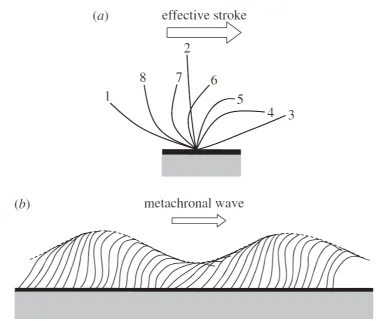
Therefore, the flow field around a micro-organism is a Stokes flow and hence the inertial force is negligible compared with the viscous force. In the Stokes flow regime, Purcell showed that the reciprocal motion cannot lead to any locomotion; (scallop theorem) [46]. However, for ciliated organisms , the motion of each in-dividual cilium follows an asymmetric pattern. First applies an effective stroke and then a recovery stroke, as we show in figure 1.1-a. The asymetry in the strokes gives to the cilium, the ability to generate a net thrust on the cell body. Cilia are typically short compared with the cell body, and the number of cilia per cell is large. A ciliate swims by synchronizing ciliary motions with slight phase differences, thus generating metachronal waves, as shown in figure 1.1-b. In the next section we shall explain in detail a simple model to take in count the ciliary motion, it is the most popular exact solution and originally due to Lighthill [35] and Blake [36].

1.4

Squirmer Model

The Lighthill [35] and Blake [36] model sometimes is referred as the envelope model, the motion of closely packed cilia tips are modeled as a continuously de-forming surface (envelope) over the body of the organism. Basically, this model consider a spherical particle with a fixed director that moves with the particlee1

ra-1.4. Squirmer Model 7

Figure 1.1: Schematic of the motion of an individual cilium and the collective motion of cilia. (a) Effective stroke of an individual cilium. The numbers in the figure indicate the order of the ciliary motion. The effective stroke is defined from 1 to 3. (Reproduced images from Ishikawa in [37].) (b) Metachronal wave generated by cilia (reproduced images from Blake and Sleigh in [47]).

dial vr and another polarvθ. Both components can be written in terms of special

functions:

ur|r=Rp =

∞

X

n=0

An(t)Pn

e1r

Rp

,

uθ|r=Rp =

∞

X

n=0

Bn(t)Vn

e1r

Rp

, (1.2)

whererrepresents the position vector with respect to the squirmer’s center, which is always pointing the particle surface and thus |r| = Rp, while e1 describes

for the n-th order Legendre polynomial and Vn is defined as

Vn(cosθ) =

2

n(n+ 1)sinθ P

0

n(cosθ). (1.3)

The amplitudes An(t) and Bn(t) determine the flow induced by the beating cilia

on the squirmer’s surface, both functions are periodic. Since the cilia wave stroke is faster than the squirmer displacement, we can replace the time dependent plitudes in the boundary conditions, eqn. (1.2), by their effective averaged am-plitudes over a stroke period, Bn(t) =Bn. Moreover, we will disregard the radial

changes of the squirming motion, An(t) = 0, in this way the velocity field

gen-erated by a squirmer will depend only in the polar part of the slip velocity and not in the size of the squirmer. Another feature in this squirmer model is that squirmer swimms in a non inertial medium hence the velocityu and pressure pof the fluid are given by the Stokes and continuity equations:

∇p=ν∇2_u,

∇ ·u= 0. (1.4)

Solving eqns. (1.4), one can then derive the average fluid flow induced by a squirmer, [48, 49]. Taking in count the boundary conditions specified by the slip velocity in the surface of its body, eqn. (1.2) and the constrains we specified above, we have that the mean fluid flow induced by squirmer is

u(r) =B1e1

−1 31 +

rr r2 Rp r 3 + ∞ X n=2 Bn

R(pn+2)

r(n+2) −

Rn p

rn

!

Pn

e₁r

r r r + ∞ X n=2

Bne1

1₋rr

r2

× nR

(n+2)

p

2r(n+2) −

(n₋2)Rn p

2rn

!

Vn e1_rr

p

1− e1r

r

. (1.5)

This solution take in count also that squirming surface has a finite total energy, given by the constrain vs = 2₃B1 along e1 where vs is the velocity in which fluid is

moving, measured in the reference system of the squirmer center of mass. With this velocity constrain we ensure that there is not net force acting on the squirmer. We are interested in study a simplified squirmer model, hence we take Bn = 0,

1.4. Squirmer Model 9

The two non-vanishing terms can model the dynamic effects associated to the squirmers. The polarity is associated with squirmer self - propulsion, through

B1, and the active stresses induced by the apolar term B2. The active stress is

quantified in terms of the squirmer self-propulsion by β = B2/B1 [48], β sign

determines squirmer behaviour, ifβ >0 squirmer behaves as puller or as a pusher if β < 0. Hence, the average fluid flow generated by this simplified model of squirmer can be written as

u(r) =−1 3

R3

p

r3B1e1+B1

R3

p

r3e1·

rr

r2

− R

2

p

r2B2P2

e₁r

r

r

r. (1.6)

Chapter 2

Lattice Boltzmann Method

In this chapter, we present the lattice Boltzmann method (LBM) which is a rel-atively new method in computational fluid dynamics. In the last 20 years, LBM has developed into an alternative and promising numerical scheme for simulating fluid flows [52]. Its strength lies however in the ability to model complex phys-ical phenomena, including single and multiphase flow in complex geometries or chemical interactions between the fluid and the surroundings.

The chapter is divided in sections, where first we make an introduction of different methods for simulate hydrodynamic interactions in soft matter, second the Boltzman equation and its discretization, in section 2.3 the Lattice Boltzmann method itself, next the boundary conditions in LBM, in section 2.5 we explain how is plugged the squirmer model in the LBM scheme, finally we explain the parallelization of our LB code and some features of it and some general conclusions.

2.1

Introduction

Microorganisms and active fluids in general, are systems where the coupling be-tween the fluid and their mesoscopic components (bacteria, active colloids, etc.) affects the dynamics of the system. The mesoscopic elements generate disturbance in the neighboring fluid which changes the fluid flow at long distances, this effect is called hydrodynamic interactions (HI).

Transport equations are used to study these kind of problems where fluid flows are taking in count. On a macroscopic scale, partial differential equations (PDE) like Navier-Stokes equation are used. Since these kind of equations are difficult to solve analytically due to non-linearity, complicated geometry and boundary con-ditions. A lot of numerical schemes such as finite difference method (FDM), finite volume method (FVM), finite element method (FEM) or spectral element method

(SEM) are used to convert the PDE to a system of algebraic equations. These macroscopic methodology is based on the discretization of the PDE. However, we can lose details of the dynamic of the mesoscopic elements.

Another approach to the problem is to consider a microscopic scale where the motion of all the particles of the system can be simulate (molecular dynamics (MD)). But we deal with the fact of the large disparity between the time-length scales of the solvent (10−10 _{s - 10}−10 _{m ) and the mesoscopic components (10}−3 _s

- 10[_{−3] m). It becomes technically impossible to reach time-length scales of the}

mesoscopic components and to simulate complex fluids as a consequence.

To close the gap between macro-scale and micro-scale, coarse-grained models have been developed. These methods reduce the degrees of freedom of the solvent but capture the collective modes of the fluid. For example, in Brownian Dynamics (BD), the solvent is represented implicitly by random forces and frictional terms. It is a simplified version of Langevin dynamics where particle inertia is neglected. BD not conserve momentum, so diffusion is present but not hydrodynamics [53]. However, another mesoscopic methods have been created, where the solvent dy-namics is explicitly resolved, for example Dissipative Particle Dydy-namics (DPD) [54, 55] where the fluid is described asN coarsened particles with continuous posi-tions and velocities. The particles interact among them by a soft potentials which leads to large time-steps and reach time scales orders of magnitude larger than the time scales of a MD. DPD was reformulated and slightly modified by P. Espa˜nol [56] to add a Galilean invariant thermostat, which preserves the hydrodynamics.

As an alternative of these mesoscopic MD-like methods we can find mesoscopic approaches based on kinetic theory. Lattice Boltzmann Method for example, it is based on microscopic models and mesoscopic kinetic equations. The funda-mental idea of the LBM is to construct simplified kinetic models that incorporate the essential physics of microscopic processes so that the macroscopic averaged properties obey the desired macroscopic equations [57].

Even though the LBM is based on a particle picture, its principal focus is the averaged macroscopic behaviour. The kinetic equation provides many of the advantages of molecular dynamics, including clear physical pictures, easy imple-mentation of boundary conditions, and fully parallel algorithms. Because of the availability of very fast and massively parallel machines, there is a current trend to use codes that can exploit the intrinsic features of parallelism. The LBM fulfills these requirements in a straightforward manner [57].

2.2. Lattice Gas Cellular Automata 13

2.2

Lattice Gas Cellular Automata

The fundamental idea behind lattice gas automata is that microscopic interactions of artificial particles living on the microscopic lattice can lead to the corresponding macroscopic equations to describe the same fluid flows.

Historically, the lattice Boltzmann method originates from the lattice gas cellu-lar automata (LGCA) which is a Cellucellu-lar Automaton (CA)1 _{where fluid particles}

are constrained to move on a regular lattice such that their collisions conserve mass and momentum. It was originally created by Hardy, Pomeau and de Pazzis in 1973 [59] known as HPP model. In this model, the lattice is square, and the particles travel independently at a unit speed to the discrete time. The particles can move to any of the four sites whose cells share a common edge. Particles can-not move diagonally. The HPP model lacked rotational invariance, which made the model highly anisotropic. This means for example, that the vortices produced by the HPP model are square-shaped [52] and it does not reproduce macroscopic hydrodynamics. Ten years after Frisch, Hasslacher and Pomeau [60] discovered that a LGCA with hexagonal symmetry, leads to the Navier-Stokes equation in the macroscopic limit (FHP model).

In general, a lattice gas automaton is a regular lattice with particles resid-ing on the nodes, all particle velocities are also discrete. So we have particles that can move around, but only within lattice nodes. The particle occupation is characterized by the occupation number

ni(x, t) ={ni(x, t), i= 1...m}, (2.1)

ni is a Boolean array, such that

ni(x, t) = 0 site x with no particles at timet,

ni(x, t) = 1 site x with one particle at timet,

(2.2)

where M is the number of velocities at each node. For example,M = 4 for HPP model, while M = 6 for FHP model.

This occupation numbers defines a M N-dimensional time dependent Boolean field, where N is the number of lattice sites [52]. The evolution of this field take place in a Boolean phase-space consisting in 2M N _{discrete states, and evolution}

equation can be written as:

ni(x+ci, t+ 1) =ni(x, t) +Ωi[n(x, t)], (2.3)

1_{Cellular automata are regular arrangements of single cells of the same kind, each cell holds}

where ci is the local particle velocity and Ωi[n(x, t)] is the collision operator. Ωi

contain all the possible collisions. Boolean nature is preserved and interactions are completely local. Configuration of particles at each time step evolves in two sequential sub-steps:

• Streaming: every particle moves to the neighbouring node according to its velocity ci.

• Collision: when there are more than one particle at the same node, they interact by changing their velocity directions according to scattering rules. The collision process is chosen so that the number of particles and the total momentum are conserved. The conservation of energy is not imposed.

Frisch et al. in [60], making use of a probabilistic approach, they considered

Ni defined as the average population at a node with velocity i. Since the average

is over a macroscopic space-time region, Ni can be written as

Ni(x, t) = hni(x, t)i, (2.4)

therefore the mean density as

ρ=X

i

Ni(x, t), (2.5)

and the mean velocity

u =X

i

Ni(x, t)ci/ρ. (2.6)

With this definitions, they have found a steady state equilibrium solution for the mean population in function of the Fermi-Dirac distribution and then they obtained a set of hydrodynamic equations that goes to imcompressible Navier-Stokes equation in the limit where the Mach number M = u√2 _→ 0 and the hydrodynamic scale L _{→ ∞}. However, some problems arise, like the lack of Galilean invariance.

2.3. Lattice Boltzmann 15

2.3

Lattice Boltzmann

The formulation of the Lattice Boltzmann Method (LBM) lies in the replacement of the Boolean occupation numbers, involved in the previous LGCA, with the corresponding ensemble-averaged populations. In this way, the artificial micro-dynamics of LGCA will be more close to the usual kinetic theory [58].

The property of the collection of particles is represented by a distribution function. That means that the Boolean occupation number ni(x, t) in LGCA is

replaced for a single particle distribution function fi(x, t), which is the ensemble

average of ni,

fi(x, t) =hni(x, t)i. (2.7)

Occupation numbernican be 0 or 1 whilefinow is a real functions with a range

0 _≤ fi ≤ 1. Therefore, a discrete kinetic equation for the particle distribution

function, which is similar to the kinetic equation in the LGCA (see eq. (2.3)):

fi(x+ci∆t, t+∆t) =fi(x, t) +Ωi[f(x, t)], (i= 0,1, ..., M), (2.8)

whereΩi =Ωi[f(x, t)] is the collision operator which represents the rate of change

of fi resulting from the collision. ∆t is the time increment. Discrete equations

like eqs: (2.8) are referred to as lattice Boltzmann equations.

Moreover, it can be shown that eq. (2.8) is a particular discretization of the Boltzmann equation [62]. Since the continuous Boltzmann equation is

∂f

∂t +v∇f =Q (2.9)

whereQ is the collision integral. We can expand the functionfi(x+ci∆t, t+∆t)

as

fi(x+ci∆t, t+∆t) =fi(x, t) +∆t

∂fi

∂t +ci∆t∇fi+O((∆t)). (2.10)

Replacing in eq. (2.8) and neglecting higher order terms:

∂fi

∂t +ci∇fi =

Ωi[f(x, t)]

∆t (2.11)

which is a correspondence to Boltzmann Equation (eq. (2.9)) where fi → f,

ci →v and

Ωi[f(x,t)]

∆t →Q.

• The particle populationsf may only move with velocities that are members of the set of discrete velocity vectorsci. The corresponding populations are

denoted fi.

• A collision operator with a single relaxation time, τ, is used to redistribute populations fi towards equilibrium values fieq . This is also referred to as

a BGK collision operator where τ is inversely proportional to density [63]. For constant density flows τ is a constant.

• The equilibrium velocity distribution function is written as a truncated power series in the macroscopic flow velocity.

Therefore, with the BGK approximation, the discrete Boltzmann equation (2.11) becomes

∂fi

∂t +ci∇fi =−

1

τ (fi −f

eq

i ), (2.12)

hence,

Ωi =−

1

τ (fi−f

eq

i ) (2.13)

and the average density, velocity and pressure tensor are given by

ρ(x, t) =

M

X

i=1

fi(x, t), (2.14)

ρ(x, t)vα(x, t) = M

X

i=1

fi(x, t)ciα, (2.15)

pαβ(x, t) = M

X

i=1

fi(x, t)ciαciβ, (2.16)

where M is the number of directions of the particle velocities at each node. Ωi

is a nonlinear collision operator, thus its evaluation is time consuming. Higuera and Jim´enez in [64] have shown that collision operator can be approximated by a linear operator, such as

Ωi(f) = Mij(fi−fieq) (2.17)

where according to [64]

Mij ≡

∂Ωi(feq)

∂fj

, (2.18)

2.4. Boundary Conditions 17

conserve mass and momentum,Mij satisfy [65]:

M

X

i=1

Mij = 0 M

X

i=1

Ωici = 0. (2.19)

Furthermore, due to eq. (2.13),

Mij =−

1

τδij (2.20)

Additionally, given the relaxation timeτ, the shear and bulk viscosity under LBM framework are

η= (2τ₋1)/6ξ = 2η/3 (2.21)

respectively [66], where we have chosen our units such that ρ= 1 for a quiescent fluid, and choose the lattice parameter (LU) as the unit of length, and the time step as the unit of time (∆t= 1), and the sound speed for the lattice in 3D that we use, cs= 1/

√

3 in LU.

Different lattice geometries, in which the distribution functions move, can be defined, specified by both the arrangement of nodes and the set of allowed ve-locities. LB models can be operated on a number of different lattices in two or three dimensions: cubic, triangular, rectangular, hexagonal, etc. A popular way of classifying the different cubic lattices is theDnQm scheme [67]. HereDnstands

for n dimensions while Qm stands form speeds.

With this basic algorithm of the LBM by using the single-time relaxation approximation and a particular Maxwell-type distribution for the equilibrium dis-tribution (eq. (8) in [68]), one can recover the Navier-Stokes equations and model single phase fluid with a variety of boundary conditions [52].

2.4

Boundary Conditions

In general, we have a great deal of temporal/spatial flexibility in applying bound-ary conditions in LBM. In fact, the ability to easily incorporate complex solid boundaries is one of the most exciting aspects of these models. LB is particularly useful in complex fluids such as suspensions of solid colloidal particles [69].

For solid boundaries we separate solids into two types: boundary solids links that lie at the solid-fluid interface and isolated solids links that do not contact fluid. With this division it is possible to eliminate unnecessary computations at inactive nodes [69].

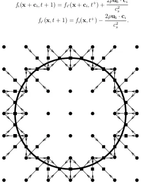
replacing the normal collision rules at a specified set of boundary nodes by the “bounce-back” collision rule [70]. This collision rule is used to model solid sta-tionary or moving boundary condition, non-slip condition, or flow over obstacles. Name implies that a particle coming towards the solid boundary bounces back into the flow domain. If we want particles to bounce back from a solid, we have to change certain values of distribution functions fi. For example, velocities f4,

f7 and f8 in a fluid node next to solid nodes (called boundary node velocity) will

pass the velocity value to the velocities f2, f5 and f6 respectively, this procedure

is schematically explained in Fig. 2.1.

Figure 2.1: Schematic illustration of bounce back rule for interaction with solids. Figure extracted from reference [71], fi vectors in the figure are the ci velocities

in the nomenclature we used along this manuscript.

2.4. Boundary Conditions 19

Ω and center of mass R, hence, ifub is the velocity in a boundary node

ub =U+Ω×

r+ 1

2ci −R

. (2.22)

By exchanging population density between a fluid node and solid node the local momentum density of the fluid can be modified to match the velocity of the solid particle surface at the boundary, without affecting either the mass density or the stress, which depend on the sum of both nodes distributions [72]. In addition to the bounceback, population density is transferred across the boundary node [72], in function of the velocity in a boundary node,

fi(x+ci, t+ 1) =fi0(x+c_i, t+) + 2ρub·ci

c2

s

fi0(x, t+ 1) =f_i(x, t+)−

2ρub·ci

c2

s

.

(2.23)

Bounce-back involves changes in the velocity distribution functions which lead to a force and torque acting locally on the fluid. The opposite force and torque are exerted on the particle. Hence, the overall fluid momentum change through bounceback determines the net force and torque acting on the rigid particle, which are used to update the particle linear and angular velocities at each time step. These velocities are then used to update the particle position and direction; the motion of colloidal particles is, hence, determined by the force and torque exerted on it by the fluid, and is resolved by a MD like algorithm [73]. With this method, we ensure a correct description of the dynamic coupling between the collective modes of the solvent and the suspended particles.

The size of the colloid is important, since due to the discretization the colloid is not strictly a sphere (as we show in Fig. 2.2), which could be relevant for the torque calculation. There are “magic” values of the particle radius, including 1.25, 2.3, 3.7, 4.77 which minimise discretisation effects [74]. Most of the results we have shown here are done with simulations with radius of 2.3 lattice units.

Again following [74], mass conservation is enforced, since when particles are near to contact they may not have a full set of boundary links with the fluid, this leads to a potential non-conservation of mass associated with the particle motion.

2.5

Squirmer model coupled to LBM

First two terms of equation (1.6) represent a dipolar field, similar to the one generated by an electric/magnetic dipole. The direction and strength of the fluid flow is specified by the polarity term B1e1 in analogy with the electric/magnetic

moments. While the B2 term models a quadrupolar field. B2 is equivalent to the

strength of a quadrupole for a symmetric arrangment of electric/magnetic dipoles, when the dipole moments vanish [75] (without polarity). Then, taking in count that we have only two non-zero terms, the boundary conditions on the surface of the squirmers depicted in equations (1.2) are written as

ur|r=Rp = 0,

uθ|r=Rp =B1V1(cosθ) +B2V2(cosθ). (2.24)

Thus, the velocity in the surface of the squirmer defined as the velocity u_|r=Rp

u|r=Rp = [B1sinθ+B2sinθcosθ]τ, (2.25)

where τ is a unit vector tangential to the surface of the particle.

2.6. Parallelization 21

equation (2.22), ub is discretized in terms of the velocities of the nodes and is

included in the bounceback rules.

2.6

Parallelization

Reason, why LBM is becoming more and more popular in the field of CFD, is the fact that LBM is solved locally. It has high degree of parallelization, hence it is ideal for parallel machines (computational clusters).

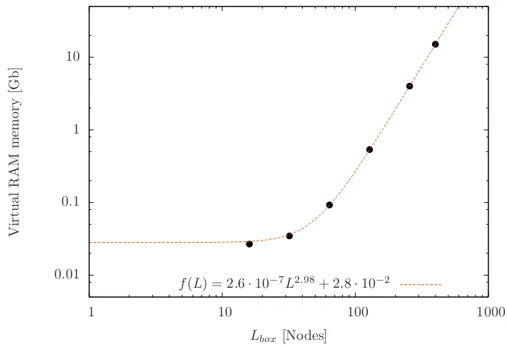
We have performed simulations using theLudwig code, which is a LB code for D3Q19 lattice [76]. It is a parallel lattice Boltzmann code which includes moving particles via domain decomposition and message passing using the message passing interface MPI, its parallelization has been tested [77]. A simulation of a fluid in a cubic box with a edge length of L= 512 lattice units, needs a RAM memory of almost 20 Gb and it the requirement of memory grows linearly with the grow of the volume, as we see in Figure 2.3.

0.01 0.1 1 10

1 10 100 1000

V

ir

tu

a

l

R

A

M

m

em

o

ry

[G

b

]

Lbox [Nodes]

f(L) = 2.6·10−7_L2.98_{+ 2.8·10}−2

2.7

Conclusions

Chapter 3

Collective motion of a squirmer

suspension

3.1

Introduction

We characterize the collective motion that emerge from active particles like spher-ical active colloids or microorganisms. We have taken in count hydrodynamic in-teractions explicitly by using Lattice-Boltzmann numerical simulations explained in Chapter 2, and active particles are modelled using a squirmer model where only two parameters are necessary to model how a microorganism swims, as described in chapter 1.

Here we study principally semi-dilute suspensions of squirmers with φ = 0.1, where φ = πσ3_N/6L3_{, σ = 2.3 and L = 120 both in lattice space units, thus}

N = 3400 for φ = 0.1. To obtain different volume fractions N was changing. We changedβsystematically to observe the emergence of collective motion depending on the hydrodynamic signature. We also show a systematic study in terms of the system size, therefore N and L were tuned to observe the effects of finite size. We set B1 = 0.01 and the viscosity ν = 0.5, therefore u∞ = 0.007 and Reynolds

number Re= 0.031.

We show that semi-dilute microorganism suspensions in 3D can develop col-lective motion and display polar alignment and giant number fluctuations. We demonstrate that both signatures of collective motion depend on the hydrody-namic properties of the particles. In particular, the emergence of giant number fluctuations is related with the formation of a macroscopic cluster. This striking phase separation emerges thanks to hydrodynamic interactions that re-orient and align the particles, and not to the reduction of velocity when local density grows. Furthermore, aligned suspensions generate a long-time super-diffusive motion

ter a cross-over from ballistic to diffusive motion generated by the re-orientation of the particles.

3.2

Collective squirmer alignment

We consider a simplified squirmer model with a slip velocity at the squirmer surface of the form

u_|r=σ

2 = [B1sinθ+B2sinθcosθ]τ, (3.1)

where τ is a unit vector tangential to the surface of the particle, θ is the angle between the direction of self-propulsion defined by the unit vectoreand the vector perpendicular to τ. B1 defines the self-propulsion speed of an isolated squirmer,

u∞ = 2/3B1 and B2 is the apolar term of the velocity and is related with the

active stresses generated by the spheres. The active stress is quantified in terms of the squirmer self-propulsion by β = B2/B1, when β < 0 squirmer it is called

pusher and puller with β > 0, while β = 0 correspond to a mover or neutral squirmer. We define a characteristic time in terms of the particle size and u∞ as

t0 =σ/u∞, whereσ is the particle diameter.

(To study squirmers, we used the Lattice-Boltzmann method (LBM), this model simulates the hydrodynamics of a liquid and shows excellent scalability on parallel computers [77], it has been successfully used to simulate squirmer suspensions in Ref. [34, 49], where the slip velocity of the squirmer, defined in Eq. (3.1), is plugged in the LBM scheme as boundary conditions (see chapter 2).

In this chapter we will concentrate on the study of semi-dilute suspensions of squirmers with volume fraction of φ= 0.1, whereφ =πσ3_N/6L3_{, the diameter of}

squirmers σ = 4.6 and the system size L = 120 both in lattice space units, thus

N = 3400 for φ = 0.1, where N the number of simulated squirmers. We have changedβsystematically to observe the emergence of collective motion depending on the hydrodynamic signature. We also show a systematic study in terms of the system size, thereforeN and Lwere tuned to observe the effects of finite size. We setB1 = 0.01 and the viscosityν = 0.5, thereforeu∞ = 0.007 and a characteristic

Reynolds number Re= 0.031.

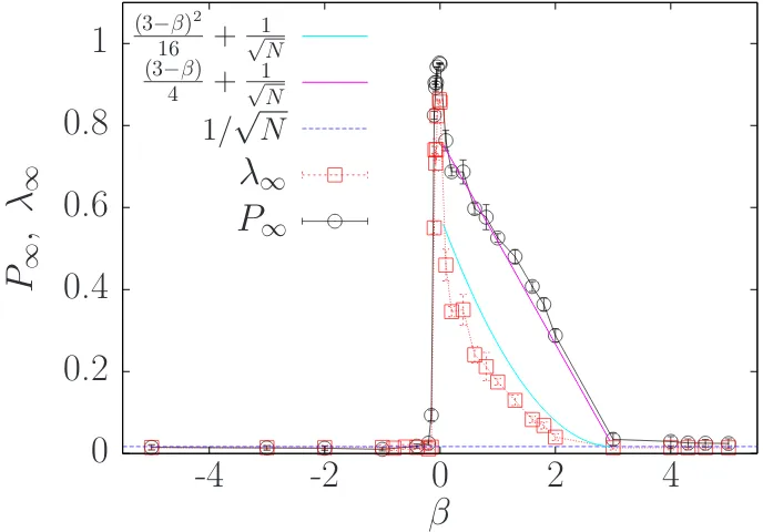
Semi-dilute squirmer suspensions can develop alignment between particles, this alignment has been measured [31, 34, 81] by the polar order parameter:

P(t) = 1

N|

N

X

i=1

3.2. Collective squirmer alignment 25

whereei is the intrinsic orientation of thei-th squirmer. At long-times, the

suspen-sion reaches a steady state P(t >>0) =P∞. IfP∞= 1 the system is completely

polarized (all squirmers pointing to the same direction), whileP∞∼1/

√

N means the system is isotropically oriented. In Fig. 3.1, the black circles show P∞ as a

function of β. Pusher swimmers withβ < ₋1/10 are isotropically oriented since

P∞ ∼ 1/

√

N, for larger values of β P∞ change abruptly, reaching values close

to 1. The suspension becomes strongly polar around β = 0, where P∞ reaches

the maximum. For pullers, β > 0, P∞ decreases with β until β ∼= 3, where P∞

saturates to ∼1/√N , like pushers with β <−1/10.

0

0.2

0.4

0.6

0.8

1

-4

-2

0

2

4

P

,

λ

β

P

λ

1/

√

N

(3−β) 4

+

1

√

N (3₋β)2

16

+

√

N

Figure 3.1: Long-time polar, P∞, and nematic order, λ∞, parameter for different

values of β, ranging from −5 to 5. P∞ correspond to black circles, while λ∞ is

represented by red squares. Particles with isotropic orientation will have P∞ ∼

1/√N hence we also show the blue dashed line for 1/√N. P∞has a roughly linear

decay in the region 0 ≤β ≤3, similarly λ∞has a quadratic behaviour in the same

region of β. Pink curve is the linear fit for P∞ while cyan curve the parabolic fit

for λ∞.

The value of P∞ is very sensitive to the system size; this reason explains the

difference with respect to the results reported in ref. [34], where P∞>1/

√

N for some pushers with β <₋1/10 at the same φ = 0.1, but withN = 2000 particles. We have verified that for an infinite system P∞ remains finite (We have done a

more detailed study on the finite size effects in section 3.7). The differences in the

P∞ here and the one shown in [34] comes from finite size effects, here the system

Since the system can have nematic order without polar order therefore, addi-tionally to the polar order parameter, we have also computed the nematic order tensor, defined as

Qhk(t) =

1

N

N

X

i=1

3

2eih(t)eik(t)− 1 2δhk

; (3.3)

for a 3Dsystem [82], wherehandkarex, y, zandN the total amount of squirmers. The nematic order parameter λ(t) correspond to the largest eigenvalue of Qhk.

Similarly to the polar order, nematic order reaches a steady stateλ(t >>0) =λ∞

that we also plot in Fig. 3.1. Red squared symbols show us that nematic order is presented for the sameβ range than polar order and for pullers withλ∞decreases

quadratically withβ untilβ = 3. We always find λ∞∼P∞2, which means that we

can consider that in semi-dilute suspensions of squirmers a polar-nematic phase emerges when−1/10≤β ≤3, and an isotropic oriented phase develops otherwise.

3.3

Number fluctuations

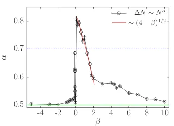
As we pointed previously [34], squirmers can develop emerging flocking and display highly dynamic, mobile flocks or clusters that can form and re-form continuously in time. These structures generate fluctuations in the number of particles. To measure these fluctuations more systematically, we calculate the number fluctu-ations for different sub-system sizes for a given β, and analyze how fluctuations h∆Nigrow with system size. We expect number fluctuations to grow as a power law of

h∆Ni ∼Nα, (3.4)

whereN is the mean of the number of particles in a given subsystem size. The fluc-tuations are proportional to √N when fluctuations are essentially uncorrelated, as is the case for systems in thermodynamic equilibrium, while active systems ei-ther experiments [83] or numerical simulations [84] have shown anomalous density fluctuations withα _≥0.75.

We have seen thatαvalue depends on theβ value as we show in Fig. 3.2 where

α is plotted for the range ₋5_≤ β _≤10. Pushers with β _{≤ −}1 have an exponent

α = 0.5, then α starts to grow slowly as we increase β until β = ₋0.1 where

3.3. Number fluctuations 27

0.5

0.6

0.7

0.8

-4

-2

0

2

4

6

8

10

α

β

∆N

_∼

N

∼

(4

₋

β)

Figure 3.2: Black circles show the exponent α obtained by fitting the number fluctuations as a power law function h∆Ni ∼ hNiα for different values of β. The green solid line is forα= 1/2, which is the case of systems in equilibrium, while the blue dashed line representα= 0.7 which is the threshold we use to define whether the system has giant density fluctuations or just anomalous density fluctuation (1/2< α <0.7).

active stresses has on the global organization of the active squirmers. Similarly, forβ = 0 the order parameters areP∞= 0.95 andα= 0.5. This abrupt change in

α is due to the fact that particles are stronger alignedP∞(β ∈[−0.01,0]) = 0.95.

Pullers on the contrary, exhibit giant density fluctuations when 0< β _≤1 and α

decays withβ as_∼(4₋β)1/2 _{up toβ = 2. Whenβ >2, we observe a slower decay}

to α = 0.5, we have reached β = 10 to get an exponent of α = 0.51. In general, we can observe in Fig. 3.2 that exponent is not symmetric with respect to β, thus pushers and pullers behave in different ways. Therefore, we observe a strong sensitivity of the number fluctuations with the character of the active stress, while pushers exhibit essentially uncorrelated fluctuations, except in a narrow region close to β = 0 where a fast increase in α is observed, pullers show a very soft transition from giant to anomalous number fluctuations up to β <3, follow by a regime where α slowly decays to 1/2.

have shown that bacterial colonies exhibit anomalous fluctuations with an expo-nent value α = 0.75±0.03 [83], while simulations of self-propelled particles with either alignment rule [86] or not [12] the scaling exponent is 0.8 for cases associated with a phase separated state.

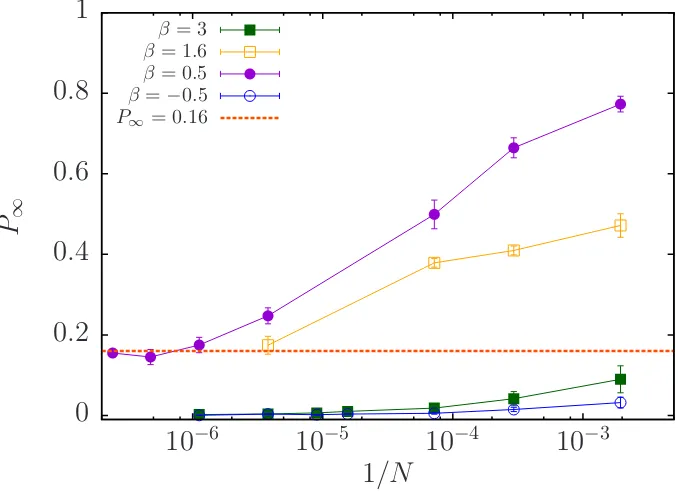
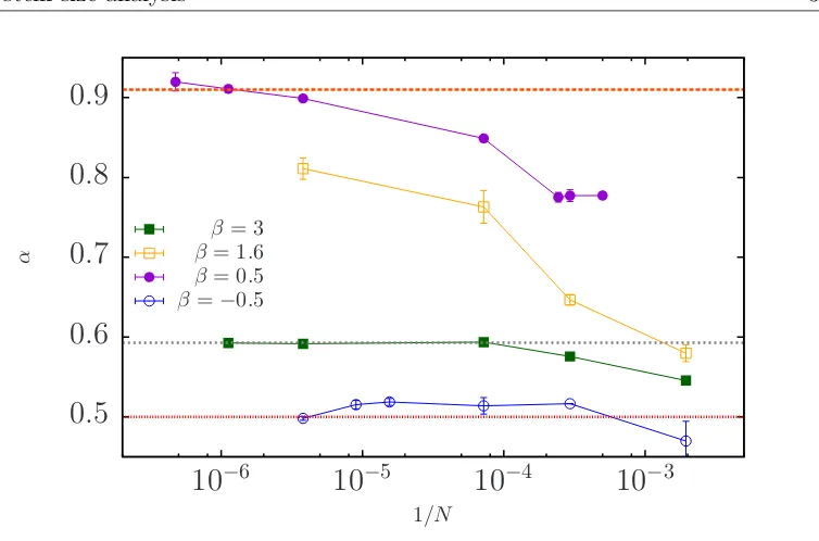
We have found that fluctuations on the density are not produced by finite size effects, on the contrary, when suspensions exhibit giant fluctuations (α >0.7), α

increases as the system size increases as we show in Fig. 3.7 reaching α ∼ 0.91 for larger systems when β = 0.5. Therefore, we found a range 0 < β ≤ 1 where semi-dilute suspensions of pullers and even pushers with ₋0.1 < β < ₋0.01 can generate giant number fluctuations, there is also a range where alignment is very high such that all particles swim in the same direction uniformly (β =_{−0.01,0_}), thus swimmers are not able to form density differences, which give us an exponent

α = 0.5. As well as pushers with β < −0.1 where particles are not aligned but the collisions between particles are uniform and the density of particles in the suspension is also uniform. While pullers withβ >1 generate anomalous number fluctuations and decay very slowly to α= 1/2 as β increases. From Figs. 3.1 and Fig. 3.2, it is clear that the alignment produced by hydrodynamic interactions is a key mechanism to have induced fluctuations.

3.4

Emergent clustering in squirmer suspension

In this section we discuss the cluster size distribution. Squirmers exhibit clustering when they reach a steady state, this steady state is characterized by a constant polar order parameter. During this interval of time we calculate the distribution of the cluster sizes.

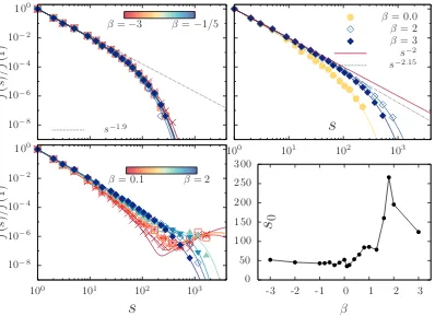
To identify the clusters we follow the methodology described in Appendix A. Once the clusters are identified, we calculate the fraction of clusters of sizes, called

f(s). We have followed the criterion elaborated by Chantal, et al. [87]: First, the range ofs-values are arbitrarily subdivided into intervals∆si = (si,max−si,min) and

estimate the total number of clusters within each interval∆si, callednti. Secondly,

we assign the value ofni =nti/∆sito everyswithin∆si. Thus, the total fraction of

cluster isNc=

P

ini∆si and the fraction of clusters of sizes,f(s) = ni/Nc, where

s is the closest integer to the central value of ∆si = (si,max−si,min). The details

of the boundaries of the clusters size intervals are explicitly shown in Appendix A. We have found that the cluster size distribution for squirmers behave in general as:

fb(s) =f(1)

exp(₋(s₋1)/s0)

sγ0 +B

exp(₋(s₋1)/z0)

s−γ0 , (3.5)

3.4. Emergent clustering in squirmer suspension 29

and distributions are completely unimodal, described by only one power law with an exponential decay given by the fitted parameters s0 and γ0. For pushers, the

exponent γ0 = 1.9 and s0 does not change significantly as β changes. CSDs for

β = ₋3 up to ₋0.2 are plotted with symbols and fitted curves to the data are plotted with lines in the top-left panel of Fig. 3.3. Similarly, B = 0 for pullers when β _≥2 and for the special case of β = 0, but γ0 = 2.15 for β ≥2 andγ0 = 2

for β = 0. In the top-right panel of Fig. 3.3 we show the CSDs for β = 0,2,3. CSDs in these cases are thicker than the CSDs for pushers showed in the top-left panel.

10−8

10−6

10−4

10−2

100 f ( s ) /f (1 )

100 ₁₀1 ₁₀2 ₁₀3

s

10−8

10−6

10−4

10−2

100

100 ₁₀1 ₁₀2 ₁₀3

f ( s ) /f (1 )

s

-3 -2 -1 0 1 2 3

s

β

s−1.9

β=₋3 β=₋1/5 β_β= 0.0_{= 2} β = 3 s−2

s−2.15

β= 0.1 β= 2

Figure 3.3: CSD of suspensions of squirmers for different β. All CSDs are fitting with an analytical bimodal distribution function of eq. (3.5). Top-left: CSDs for pushers. Top-Right: CSDs for β = 0,2,3. Bottom-left: CSDs for pullers in the range 0< β_≤2. Bottom-right: Parameter s0 as a function of β.

Cluster-size distributions of pullers with 0 < β < 2, exhibit a bimodal be-haviour, like the eq. (3.5) with B ₆= 0, when 0 < β _≤ 1 the exponent γ0 = 2.2

and prefactor B _∼ 10−13 _{with the exponential cutoff z}

0 ∼ 1000 (reddish curves

in bottom-left panel of Fig. 3.3) while the range 1 < β < 2 has an exponent

γ0 = 2.075 and prefactor B ∼10−10 with z0 ∼100 (blueish curves in bottom-left

panel of Fig. 3.3). The exponential cut-off s0 is plotted in the bottom-right panel

value around 50, while for pullers s0 grows slowly whenβ < 1 and then it grows

faster, until a maximum of s0 = 266 at β= 1.8.

The bimodal cluster-size distributions observed for pullers withβ ≤1 (reddish curves in bottom-left panel of Fig. 3.3) reach cluster-sizes arounds∼1600 parti-cles, which is approximately half of the total amount of particles in the suspension. These clusters can be seen as macroscopic clusters.

3.5

Density-dependent speed

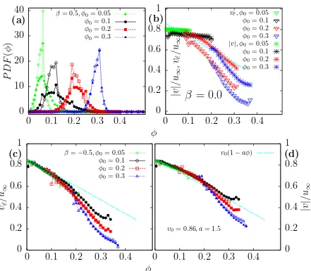
Although the macroscopic clusters, generated by someβs, can be understood as a phase separated state, the nature of this phase differs from the MIPS scenario [16], when macroscopic phase separation emerges as a result of a decrease of particle motility with concentration. In order to identify if hydrodynamic interactions can induce effective decrease in squirmer motility that can, indirectly, lead to the appearance of the macroscopic clusters reported, we have computed the local volume fraction for squirmers withβ =₋1/2,0,1/2.

The local volume fraction is calculated at the center of every particle in the system. Where we estimate the number of particles around every particle inside of a typical cut-off distance. The cut-off distance we have used is 3σ whereσ is the diameter of the particles. Although the choice of the cut-off distance is arbitrary, from a systematic study, we have observed that either the probability distribution of the volume fraction or the density dependent speed does not depend on the cut-off distance, when the distance between 2σ and 4σ.

In Fig. 3.4a we show the probability distribution P DF(φ) of the local vol-ume fraction for two types of squirmers, pullers with β = 0.5 (solid symbols) and pushersβ =₋0.5 (hollow symbols). Green diamonds correspond to the probabil-ity distributions for suspensions with a total volume fraction of φ0 = 0.05. For

pushers the probability distribution ranges from 0 to 0.1, while pullers spread up toφ = 0.2. The increase in the range of local values of φ is due to the emergence of large clusters in the system. Similarly, when the average volume fraction is

φ0 = 0.1 (black symbols) pushers have a narrow distribution center in φ = 0.1

while pullers have a wider distribution in which the local volume fraction fluctu-ates from 0 to 0.35, pullers with β = 0.5 and φ0 = 0.05 or 0.1 are suspensions

where the macroscopic cluster emerges,

3.5. Density-dependent speed 31

0

10

20

30

40

0

0.1

0.2

0.3

0.4

P

D

F

(

φ

)

(a)

0

0.2

0.4

0.6

0.8

1

0

0.1

0.2

0.3

0.4

|

v

|

/u

,v

/u

φ

β

= 0.0

(b)

β = 0.5, φ0= 0.05

φ0= 0.1

φ0= 0.2

φ0= 0.3

veˆ, φ0= 0.05

φ0= 0.1

φ0= 0.2

φ0= 0.3

|v|, φ0= 0.05

φ0= 0.1

φ0= 0.2

φ0= 0.3

0

0.2

0.4

0.6

0.8

1

0

0.1

0.2

0.3

0.4

v

/u

∞

(c)

0

0.1

0.2

0.3

0.4

0

0.2

0.4

0.6

0.8

1

|

v

|

/u

φ

v0= 0.86, a= 1.5

(d)

β =−0.5, φ0= 0.05

φ0= 0.1

φ0= 0.2

φ0= 0.3

v0(1−aφ)

Figure 3.4: (a) Distribution profiles of the local densities for β = ±0.5 with different values of global density. Solid symbols are for pullers with β= 0.5 while hollow symbols for pushers with β = −0.5. (b) Density-dependent speed |v(φ)| and velocity projected to the orientational vector vˆe(φ) for squirmers with β = 0.

Hollow triangles are vˆe(φ), stars are |v(φ)| and each color correspond to different

total density φ0. (c) Density-dependent velocity projected to the orientational

vector vˆe(φ) for β = ±0.5 . (d) Density-dependent speed |v(φ)| for β = ±0.5.

All velocities are normalized by the asymptotic swim speed of a single squirmer

u∞ = 2/3B1. Color and symbols maps are the same for (a),(c) and (d). Pullers

are solid symbols, while pushers are hollow symbols.

particles accumulate in regions where they move slowly and it causes further ac-cumulation of particles. This motility-induced phase separation occurs without attractive interactions or orientational order and it has been confirmed in sim-ulations [12, 13, 16], experiments [96] and by a continuum description for the structural evolution [16]. Given this theoretical framework, they have found that velocity dependent linearly with the density. In the cases of squirmers, where hydrodynamic interactions are taking in count, we have found that the system density affects the local particle motility, as we observe in Fig. 3.4b where the density-dependent speed |v(φ)| and the velocity projected to the orientational vector of squirmers vˆe(φ) changes as the concentration regime changes forβ = 0.

For semi-dilute cases with φ0 = 0.05 and 0.1, both velocities do not depend on

the local density, since all the suspension is aligned, although all particles move in the propulsion direction _|v(φ)_|=veˆ(φ) this speed is less than u∞= 2/3B1, due to

the hydrodynamic field generated by neighbour particles. For a more concentrate case where φ0 = 0.2 or 0.3, speed and projected velocity depend on the local

density and motility is reduced as local density increases. Forφ0 = 0.2|v(φ)| and

veˆ(φ) follow a linear behaviour in their range of local densities where values are

more relevant statistically. While φ0 = 0.3 case follows an asymptotic decay to

a non-zero value. Which tell us that particles always move even for concentrated regimes where local density can reach values up to φ= 0.35. Another important remark is the difference between the value of the speed and the projected velocity. Speed is always greater than projected velocity for a given density. This contrast correspond to the hydrodynamic flow around the particle that contributes to the total speed of the particle.

For squirmers with β = ±0.5, the velocity along the self propelled direction decays as a function of the local density as we observe in Fig. 3.4c, regardless of the average volume fraction. For φ0 = 0.05 (green diamonds), for both pushers

and pullersvˆe(φ) decays linearly untilφ = 0.15 according to the cyan curve in Fig.

3.4c, then both cases decay faster, where pushers decay even faster than pullers due to the partial alignment of pullers. The same behaviour is found at higher volume fractionφ0 = 0.1 (black circles). On the contrary, for denser systems with

total volume fraction of φ = 0.2 projected velocity for either pushers or pullers decays almost in the same way, a tendency even more clearly seen at φ = 0.3.

|v(φ)| for β = ±0.5 plotted in Fig. 3.4d, follows the same pattern than pro-jected velocity. But as in β = 0.0, the speed taking in count the velocity induced to the particle by hydrodynamic flows around the particles. Thus, speed is greater than projected velocity for a given local density.

3.6. Mean Square Displacement 33

well defined coexistence densities [16], while theP DF(φ) for squirmers has a uni-modal shape, where the thickness of the distribution depend on the hydrodynamic signature. When macroscopic clusters appears, the P DF(φ) is wider than other cases, this cluster is very dynamic and form and re-form very fast, therefore this loose cluster can not form a binodal state, like MIPS for active brownian particles in [16].

On the other hand, swim speed is affected by hydrodynamic interactions, since density-dependent speed changes asβchanges. When squirmers are highly aligned with β = 0 and φ ≤ 0.1 both velocities do not change as local density change, otherwise velocities decay as density increases. This behaviour is due to the col-lisions as in ABPs, however squirmers do not follow a linear behaviour. We have also found that pullers with macroscopic clusters generate non-zero velocities, de-caying very slow to zero at high density due to the orientational order, whereas the velocities of pushers and squirmers with higher average density decay faster to zero.

3.6

Mean Square Displacement

We want to analyse the squirmer dynamics as a function of their activity. In particular, we want to understand the impact that the global polarization observed for pullers has on squirmer motion. To this end, we concentrate first in the Mean Square Displacement (MSD) defined as

∆r2(t)

= 1

N

N

X

i=1

[~ri(t)−~ri(0)]2, (3.6)

WhereN is the total amount of squirmers in the suspension. In Fig. 3.5a we show the MSD for squirmers such as orientational order is absent, MSDs evolve from a initial ballistic regime to a linear one. Thus, we are able to determine the diffusion coefficient, by calculating the slope of the MSD at long-times, since according to the Eistein relation:

h∆r2_(t)i

σ2 = 6D

t t0

, (3.7)

where σ is the diameter of the squirmer, t0 the time that a squirmer needs to

travel one diameter at velocity u0 = 2/3B1 and D the diffusion coefficient. We

100

102

104

106

100 ₁₀1 ₁₀2 ₁₀3

h

∆

r

2(t

) i /σ 2 t/t0 (a) 100 101 102

-4 -2 0 2 4

D

β β=−3

β=−2

β=−1

β=−0.2

β= 3

100

102

104

106

108

100 ₁₀1 ₁₀2 ₁₀3 ₁₀4

h ∆ r 2( t ) i /σ 2 t/t0

∼t2

∼t2

(b)

β= 2

β= 1

β= 0.5

β= 0.0

β=−0.1

Figure 3.5: (a) Mean-squared displacement for squirmers without alignment, lines correspond to a linear fitting at long t when diffusive regime (∆r2_{(t) ∼ t) is}

present. Inset: Diffusion coefficient as a function of β. D is only defined when suspension has a diffusive behaviour. (b) Mean-squared displacement for aligned squirmers for β between ₋0.1 _≤ β _≤ 2. Orange solid line describe the ballistic regime.

times (Fig. 3.5b), the evolution of the MSD to a super-diffusive regime is a consequence of the hydrodynamic field generated by the squirmers.

In Fig. 3.5a MSDs evolve to a diffusive regime at t >102_t

0 and remain in this

regime, whereas in Fig. 3.5b MSDs evolve to a transient diffusive regime follow by a crossover to a steady super-diffusive regime.

The precise time where the crossover to diffusive regime occurs will depend on

β. The greater the value of|β|the shorter the time to diffusive regime. Similarly, the time of crossover to super-diffusive regime also vary with β. The time that squirmers spend in the transient diffusive regime coincides with the time that polar order needs to reach the steady state where P(t) =P∞.

3.7

System size analysis

Given the proven accuracy of the Ludwig code [77] we are able to reach 3D periodic systems with edge length up to 1280 node-node distance, thus we have studied semi-dilute squirmer suspensions with a total number of particle up to_∼4_×106_.

3.7. System size analysis 35

3.7.1

Polar Order

We show that polar order decrease with the system size, but it reaches an asymp-totic value at large N. When β = 0.5 (purple circles in Fig. 3.6) P∞ goes from

0.77 at N = 514 to an asymptotic value of 0.16 when N _≈ 106_{. Analogously, at}

β = 1.6 P∞ drop from 0.47 to 0.17 when N = 263500, in this case we can not

conclude whether the polar order goes to zero or to a constant value as β = 0.5 (yellow squares in Fig. 3.6). But, for cases where P∞ ≈ 1/

√

N at N = 3400 like pushers with β = −0.5, or pullers with β = 3 they still have the 1/√N

dependency as the system grows, as we show in (blue circles and green squares in Fig. 3.6). The general drop in the long-time polar order that we observe for the different values of β as the system size grows, explain why Ishikawa et al. in [30] and Evans et al in [31] have reported higher values of the polar order for different values ofβ, since they have used systems with N = 64 particles, whereas us in [34], we have used N = 2000 in which there is a higher value of P∞ in

comparison with Fig. 3.1 where we have used N = 3400. Additionally, Delmotte

0

0.2

0.4

0.6

0.8

1

10

10

10

10

P

1/N

β= 3 β = 1.6 β = 0.5 β=−0.5 P∞= 0.16

Figure 3.6: Long time polar order as a function of the system size for differentβs.