Essays on the economics of culture and identity

(1)

Essays on the Economics of Culture and

Identity

Vasiliki Fouka

TESI DOCTORAL UPF / ANY 2015

DIRECTOR DE LA TESI

Prof. Hans-Joachim Voth

(2)

(3)

(4)

(5)

ACKNOWLEDGEMENTS

I would first like to thank my advisor, Hans-Joachim Voth, for his constant support and mentoring over the last five years. He has been for me an invaluable teacher, not just of research skills, but also, and most importantly, of those non-cognitive skills and attitudes so necessary for the completion of a PhD, for working in academia and for life in general: trust in one’s self, perseverance and the habit of thinking broadly, before solving the inevitable constrained optimization problems. The comments of my readers, Albrecht Glitz, Stelios Michalopoulos and Luigi Pascali were crucial for turning my research proposal to a completed thesis. I am indebted to Ran Abramitzky, Alberto Alesina and Davide Cantoni for their comments on the job market paper. I also owe thanks to Nathan Nunn for hosting me at Harvard for a year.

I would like to thank seminar participants in Brown, Harvard, Lucerne (SEA), Naxos (CRETE), Northwestern, NYU (NEWEPS3), Stanford, Toulouse (ESEM), UPF and Vanderbilt for their constructive feedback on different chapters of the dissertation.

A big thanks to Marta Araque and Laura Agust´ı, for their accessibility and efficiency, which made every administrative step of the PhD easier.

Thank you to Tanya, Bruno, and Ciccio, for sharing with me an office and six long years at UPF. To Andrea, Felipe and J¨org for sharing the preparation for the job market, to Thomas for his good energy and for always being a trustworthy hiking buddy and to all my fellow UPF students. Corina, Andreas, Egemen, Laura, Dileimy and Vicky, thank you for being great flatmates and friends and my window to the outside world.

I owe so much to my family and friends, in Spain and in Greece, for being there for me throughout the PhD. A thank you to my parents, Nikos and Fotini and my brother, Xenophon, whose programming skills proved particularly useful for part of this thesis.

(6)

(7)

Abstract

This thesis examines how culture — in the sense of identity and preferences — re-lates to economic decision-making. The first chapter investigates how a prohibition of their native language in school affects the assimilation of German immigrants in the US in the early 20th century. I find that restrictive language policies pro-duce a backlash of ethnic identity, which is particularly pronounced among less assimilated immigrants. In the second chapter I examine the role of history and memory in shaping consumer decisions. I show that the share of German car sales in Greece drops during periods of conflict between the Greek and German gov-ernments, and that this drop is larger in areas of the country which suffered from German reprisals during World War II. The third chapter provides a theory on the origin of the preference for work. Combining agroclimatic and attitudinal survey data from Europe, I show that regions in which returns to labor in agriculture have historically been high place more value on work versus leisure today.

Resumen

(8)

(9)

PREFACE

Until recently, culture — in the sense of preferences, collective beliefs and social norms formed through parental socialization and history — featured very little in the topics of interest of economists. The vagueness of its definition, and the reluctance of the discipline to touch fundamentals of economic models such as preferences, left the study of culture to other social sciences, better equiped to deal with it, such as psychology or anthropology. Owing to Greif (1994), and after him Akerlof and Kranton (2000) and Bisin and Verdier (2000), economists not only started developing ways of thinking about culture, but also managed to show that economic models are a good way of understanding how culture is both shaped by the economic environment and is itself a driver of economic behavior.

Despite the burgeoning literature that ensued on the study of culture, we still have a long way to go in understanding where culture comes from and how it matters for economic outcomes. Empirically identifying the roots of attitudes and norms, or isolating their effects on behavior from other proximate factors is challenging. A number of studies document convincingly the persistence of culture over very long periods of time. But what makes this persistence weaken, and when the effect of history on behavior becomes more or less pronounced is relatively less understood.

(10)

produce a backlash of German ethnic identity, particularly for individuals coming from homogeneous German families. These German-Americans were more likely to marry within their ethnic group and choose decidedly German names for their offspring. They were also less likely to volunteer in the US Army during World War II. This backlash effect is more pronounced in places with a small German minority and places where the initial sense of German identity, as proxied by the strength of the Lutheran church and the presence of Lutheran parochial schools, was stronger. These results are compatible with a model of cultural transmission of identity, in which parental investment overcompensates for the direct effects of assimilation policies.

In the second chapter, coauthored with Hans-Joachim Voth, I investigate how historical memory affects consumer choices in the context of the Greek debt crisis. Combining an index of political sentiment constructed from over 60,000 newspaper articles with historical maps on German war crimes in Greece during World War II, we find that German car sales drop in response to German-Greek political acri-mony, especially in areas with a memory of past German atrocities. We conclude that cultural aversion was a key determinant of purchasing behavior, and that memories of past conflict can affect economic choices in a time-varying fashion. These findings are compatible with behavioral models emphasizing the importance of salience for individual decision-making.

(11)

(12)

(13)

List of Figures

1.1 Language laws, 1917–1923 . . . 10 1.2 Counties on the northern and southern borders of Indiana and Ohio 20 1.3 Balancedness of border data set . . . 23 1.4 Locations of linked data set in 1920 . . . 25 1.5 Densities of log GNI of first son by cohort . . . 36 1.6 Difference in Germanness of first name by birthplace of parents . . 43 1.7 Ethnic composition and effects of the language ban . . . 47 1.8 Strength of ethnic identity and effects of the language ban . . . 49 1.9 Schools of the Lutheran Church-Missouri Synod in 1913 . . . 50 1.10 Match rate for border data set, by cohort and language law status . 60 1.11 Cumulative distribution function of the GNI in the 1930 IPUMS by

gender and German origin . . . 61 1.12 GNI density by gender: Children in border data set . . . 62 1.13 Correlation of German names with gender and birth order . . . 63 1.14 Match rate for WWII enlistments, by cohort and language law status 64 1.15 1942 enlistments and volunteers by birth cohort . . . 65 1.16 Endogamy rates of second-generation Germans in IPUMS sample . 66 2.1 Changes in the market share of German cars . . . 76 2.2 Map of towns affected by German reprisals, 1941–1944 . . . 81 2.3 Number of international news articles referring to German-Greek

(18)

2.7 Comparison of news and search-based conflict index . . . 104

2.8 Facebook membership in boycott groups . . . 109

2.9 German-Greek conflict and evolution of German market share in prefectures with and without reprisals . . . 114

2.10 Decline in the market share of German cars . . . 123

3.1 Potential labor intensity in the regions of Europe . . . 136

3.2 Potential labor intensity and historical hours worked . . . 137

3.3 Bivariate correlation plots . . . 138

(19)

List of Tables

1.1 Balancedness of border counties . . . 21

1.2 Summary statistics: Border data set . . . 24

1.3 Most and least German-sounding names in the 1930 census . . . 27

1.4 Summary statistics: WWII enlistments . . . 30

1.5 Baseline results: Border data set . . . 35

1.6 Baseline results: WWII enlistments . . . 39

1.7 Non-German mothers: Border data set . . . 42

1.8 Non-German mothers: WWII enlistments . . . 45

1.9 Proximity to Lutheran schools . . . 51

1.10 Educational and labor market outcomes . . . 53

1.11 Endogamy in IPUMS . . . 56

1.12 Summary of legislation enacted 1917–1923 . . . 67

1.14 Summary statistics: Non-German mothers, border sample . . . 68

1.13 Characteristics affecting the probability of a match: Border data set 69 1.15 Characteristics affecting the probability of a match: WWII enlist-ments . . . 70

1.16 Summary statistics: Non-German mothers, WWII enlistments . . . 71

2.1 Chronology of Greek crisis and German-Greek conflict month iden-tification . . . 86

2.2 Monthly car registrations in Greece . . . 89

2.2 Monthly car registrations in Greece (cont.) . . . 90

2.3 Summary statistics of main variables . . . 92

2.4 Balancedness . . . 93

(20)

2.6 Share of German cars, baseline . . . 98

2.7 Sample subdivision . . . 101

2.8 Alternative measures of German-Greek conflict . . . 103

2.9 Alternative definitions of reprisals . . . 106

2.10 Assessing selection on unobservables . . . 107

2.11 Effects by membership in Facebook boycott groups . . . 110

2.12 Triple differences . . . 112

3.1 Estimates of crop-specific labor shares from Prussian agricultural data . . . 135

3.2 Individual-level OLS estimates using data from EVS and ESS . . . 140

3.3 Individual-level OLS estimates for natives using EVS and ESS data 141 3.4 Weekly hours worked for children of European immigrants in the US 142 3.5 Regional-level estimates using data from EVS and ESS . . . 144

3.6 Potential labor intensity estimated with US data . . . 145

3.1 EVS Sample . . . 154

3.1 EVS Sample (cont.) . . . 155

3.2 ESS Sample . . . 155

3.2 ESS Sample (cont.) . . . 156

(21)

Chapter 1

BACKLASH: THE UNINTENDED

EF-FECTS OF LANGUAGE PROHIBITION

IN US SCHOOLS AFTER WORLD WAR I

1.1 Introduction

From France’s “burkha ban” to the politics of bilingual education in California, societies around the world grapple with the challenge of integrating ethnic minori-ties. Theories of nation building (Alesina and Reich, 2014) assume that policies such as imposing a national language or otherwise repressing minority culture will lead to more homogeneity. At the same time, one strand of literature has shown theoretically that identity may be strengthened in the face of policies aimed at integration (Bisin and Verdier, 2000, 2001; Bisin et al., 2011). What is unclear is when assimilation can work in practice, and what drives the risk of a backlash.

(22)

it contribute to a cultural backlash and greater isolation from the mainstream of American culture? To guide the empirical analysis, I construct a simple model of intergenerational transmission of ethnic identity. I derive conditions under which a cultural backlash is more likely. Using a variety of data sources — including linked census records and World War II enlistments — I examine several outcomes for German-Americans affected by language restrictions: (i) their intermarriage rates, (ii) the ethnic distinctiveness of the first names chosen for their offspring, and (iii) their decision to volunteer for the US Army during World War II.

I exploit both within–cohort variation (comparing states with and without a German ban) and within–state variation (comparing cohorts at school with older cohorts) in a difference–in–differences (DiD) model. I find a strong backlash effect for the children of German immigrants and this effect is consistent across outcomes and specifications. Treated cohorts in this group are 1–8 percentage points more likely to marry endogamously (i.e. within their ethnic group) and 10–12 percentage points less likely to volunteer in 1942. They also choose more distinctively German names for their children, with the estimated effect being equivalent to switching from a name like Chris to a name like Adalbert.

(23)

In accordance with this dynamic, I also find a greater backlash among those liv-ing closer to Lutheran parochial schools; such individuals were likely to sort there owing to their preference for ethnic schooling.

My findings imply that linguistic immersion through the prohibition of Ger-man has no clear assimilation effect on average. Instead, and across all outcomes, a language ban leads to a robust increase in the spread between individuals of uniform and mixed German ancestry. Furthermore, I find that the language ban has no significant effect on years of schooling and is thus unlikely to influence assimilation outcomes through its effect on education. I do, however, find evi-dence that a strengthening of ethnic identity entails a penalty for individuals who become more German. German-Americans with two German parents affected by language laws experienced an earnings penalty in the labor market. Given that schooling outcomes are unaffected, such a drop in earnings is unlikely to be due to lower quantity or quality of education as a result of linguistic immersion. It is, however, consistent with research emphasizing the economic payoffs of assimilation (Biavaschi et al., 2013).

(24)

study of German-Americans yields an interesting measure of ethnic identification: volunteering for service in the US Army during World War II. This is a unique historical setup in which immigrants are called upon to take sides between their host country and their country of origin; as a proxy of assimilation, that decision is very little contaminated by economic or other confounding factors.

The paper proceeds as follows. Section 1.2 relates this work to the existing literature. Section 1.3 discusses the historical background of German language schooling and the language restrictions imposed after WWI. Section 1.4 presents a simple model of cultural transmission used to examine the implications of a shock on ethnic schooling for the ethnic identity of children belonging to a minority. Section 1.5 describes my data sources. Section 1.6 is devoted to the empirical analysis. I show that the prohibition of German in school created a backlash of ethnic identity among Americans born to German parents, as measured by en-dogamy rates, ethnic name choices and volunteering in World War II. Section 1.7 shows how this backlash effect weakens among children of mixed couples and as-sesses how the response to legislation varies by a community’s ethnic composition and strength of ethnic identity. Section 1.8 examines whether language restrictions affected schooling outcomes and verifies that language laws had a similar impact in the US as a whole as they did in the restricted set of states I examine. Section 1.9 reviews my findings in the context of recent theory on cultural transmission and identity in economics. Finally, Section 1.10 concludes.

1.2 Relation to existing literature

(25)

the school. Bisin et al. (2011) present a mechanism for the persistence of opposi-tional minorities.1 _{In their model, oppositional types intensify their identification}

with the minority culture in response to attempts at desegregation or discrimi-nation by mainstream society. Similarly, Carvalho (2013) predicts that bans on veiling worn by Muslim women can increase religiosity.

My paper relates to a broad literature on immigrant assimilation. Much of this research has focused on economic assimilation and the gap between native and immigrant earnings.2 _{In addition, several papers construct measures of the}

speed of assimilation by looking at political (Shertzer, 2014) or cultural outcome variables (Aleksynska and Algan, 2010), such as first names (Arai et al., forth-coming) or self-reported national identity (Manning and Roy, 2010). D´avila and Mora (2005), Neeraj et al. (2005), and Gould and Klor (forthcoming) show how discrimination against Muslims in the United States after the 9/11 attacks reduced integration. My study contributes to this literature by identifying the effect of a specific government intervention on assimilation outcomes.

My research also contributes to the literature on the economics of identity (Akerlof and Kranton, 2000). Identity has been shown to explain a variety of economic outcomes, including risk and intertemporal choice patterns (Benjamin et al., 2010), contributions to public goods (Benjamin et al., 2013), as well as educational decisions (Austen-Smith and Fryer, 2005), but evidence on the deter-minants of identity formation is generally not causal in nature (Constant et al., 2009; Nekby and R¨odin, 2009; Battu and Zenou, 2010; Manning and Roy, 2010; Bisin et al., 2013).

More broadly, this paper relates to a rich literature in history, economics, and sociology that examines the effects of education on national identity. There are many studies documenting how education and the content of the school curricu-lum have been used to shape preferences, homogenize societies, and “manufacture” nations (Dewey, 1916; Freire, 1970; Weber, 1976; Colley, 1992). More recently in the economics literature, Cantoni et al. (2014) show how a new school curriculum in China had a measurable effect on the political attitudes of students. My study

1_{See also Bisin and Verdier (2000), Bisin and Verdier (2001) and Bisin et al. (2004).}

2_{See Borjas (1985), LaLonde and Topel (1991), Hatton (1997), Minns (2000), Card (2005)}

(26)

focuses more on the medium than on the content of education, but its results sug-gest that the purpose of integrative educational policies is seldom entirely achieved. The study of Friedman et al. (2011) in Kenya points in a similar direction. They find that more education in the context of a nationalist curriculum led to political alienation for school girls, especially those not belonging to the country’s leading tribe.

Relative to the existing literature, I make the following contributions. My paper is the first to provide empirical evidence on the existence of a backlash of identity in response to assimilation policies. Second, I test the relevant mechanism driving this reaction: cultural distinction, or the tendency of parents to invest more in enculturating their children when there are few role models among their children’s peers. Finally, I contribute to the literature on identity formation by providing evidence on a specific mechanism through which ethnic identity can be influenced: language in school and its interaction with parental socialization. In this regard, the paper most closely related to mine is Clots-Figueras and Masella (2013).3

1.3 Historical background

This section outlines the history of the German language in US schools until the early 20th century. It also discusses the reasons that led to the restriction of German as a language of instruction during and after World War I.

1.3.1 Germans in the United States and the German

lan-guage in schools

Germans were the single largest foreign group that migrated to the post-colonial United States until at least the 1970s. Starting in the 17th century, German immigration increased as a result of the mid–19th-century political upheavals in Europe and peaked in 1890, when economic migrants replaced political refugees

3_{These authors find that instruction in Catalan, which was re-introduced in the schools of}

(27)

in the arriving immigrant cohorts. Between 1880 and 1920, Germans were always the largest element among the foreign-born in the United States; in 1900, the first and second generation of Germans together constituted little more than 10% of the total US population (Conzen, 1980).

As the dominant non–English speaking group, Germans established a large network of private (mainly religious) schools, in which the German language was taught and used as a medium of instruction; they also succeeded in introducing German instruction to the public schools of districts with a large German popu-lation. In cities such as Cincinnati and Indianapolis, designated German-English schools provided a form of bilingual education that included daily half-day instruc-tion in German (Schlossman, 1983; Zimmerman, 2002). Such bilingual programs were favored by German parents and they were also supported by school officials as a way of drawing first- and second-generation German children away from private schools, which were perceived to perpetuate exclusive ethnic communities and to endanger the linguistic and cultural homogenizing function of the public school. Some proponents of dual German-English instruction pointed out its assimilating function not just for the children of German immigrants but also for their par-ents. According to the Milwaukee Association of Collegiate Alumnae: “Foreign mothers, who are busy all day in their homes, have but one opportunity to acquire the language of their adopted country, and that is from their children, who bring English home from the schools” (Schlossman, 1983).

Although there is no comprehensive census of private schools and their instruc-tion practices, individual state census records reveal the prevalence of German in parochial schools prior to World War I. According to the 1917 Minnesota Educa-tional Census, the state counted 308 parochial schools with a total enrollment of 38,853 pupils; more than two thirds of these schools used both German and English as a medium of instruction (Rippley, 1981).4 _{Official statistics aside, a number of}

sources confirm the unofficial use of German by teachers in the classroom as a nat-ural way of introducing first- and second-generation children of German parents to English (Schlossman, 1983). For parochial schools that employed German-born teachers and were located in predominantly German rural communities, this

prac-4_{In the early 20th century, 35 out of 48 states taught some form of German in school mostly}

(28)

tice was the norm.

Despite this ethnic group’s large network of schools, the prevalence of using German and the importance placed by German-Americans on conserving their culture and a sense of Deutschtum, by the early 1900s Germans were fairly well assimilated — in both socioeconomic and cultural terms — into US society. In the words of Higham (1998), “public opinion had come to accept the Germans as one of the most assimilable and reputable of immigrant groups. Repeatedly, older Americans praised them as law-abiding, speedily assimilated, and strongly patriotic.”

1.3.2 WWI, anti-Germanism, and language restrictions

The outbreak of the First World War made the large German community the focus of American patriotic reaction. The growing anti-Germanism of the early war years, which was further agitated by the insistence of the German-American press on strict American neutrality, found its expression in a series of both spontaneous and organized acts of harrasment and persecution once the United States entered the war in 1917. Numerous German-Americans were arrested as spies or forced to demonstrate their loyalty by buying liberty bonds under the threat of vandalism or tarring and feathering. The hanging of Robert Prager in Collinsville, Illinois, was the most well known in a series of lynching attacks against German-Americans (Luebke, 1974). Berlin, Michigan, was renamed to Marne in honor of the American soldiers who fought in the Second Battle of Marne. Hamburgers became “liberty steaks”5 _{and sauerkraut consumption fell by 75% in the period 1914–1918 (New}

York Times, 25 April 1918). Moser (2012) shows that the number of German-language operas featuring in the New York Metropolitan Opera fell dramatically during the war years.

The German language also came under attack. At the federal level, the 1917 Trading With The Enemy Act and also the Espionage Act required all foreign language publications to translate into English any news referring or related to the war. At the state and local level, various restrictions were placed on the

5_{An interesting parallel is the renaming of french fries to “freedom fries”, after France opposed}

(29)

use of German. The state of Iowa prohibited, among other things, the use of German over the telephone. Iowa state governor William Lloyd Harding stated in the New York Times in June 1918 that “English should and must be the only medium of instruction in public, private, denominational and other similar schools. Conversation in public places, on trains, and over the telephone should be in the English language. Let those who cannot speak or understand the English language conduct their religious worship in their home” (Baron, 1990).

This political climate encouraged support for language restrictions in the schools. Since the war’s outbreak, nationalist organizations had propagandized against the instruction of German. A 1915 pamphlet of the American Defense League, one of the largest nationalist political groups of the time, reads as follows: “Any lan-guage which produces a people of ruthless conquistadores [sic] such as now exists in Germany, is not fit to teach clean and pure American boys and girls.” This pro-paganda merged with a pre-existing nativist movement that originated in the 19th century, but had strengthened in the early 1900s in response to the unprecedented flow of immigration to the United States (Kazal, 2004). During and after the war years, these attitudes were enshrined in legislation restricting foreign languages in a number of states.

(30)

[image:30.595.144.493.132.366.2]

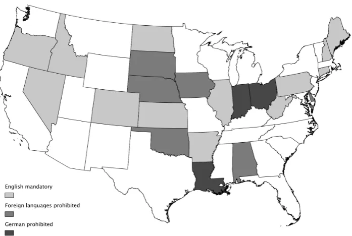
Figure 1.1: Language laws, 1917–1923

Notes: Data from Edwards (1923).

World War I marks a clear break in the pre-existing trends of English language legislation; in the period 1917–1923, there were 21 states that prohibited the use of foreign languages as a medium of instruction or as a separate subject in elementary grades (Knowlton Flanders, 1925). Figure 1.1 depicts these states in terms of the type of law they introduced. Though not always explicitly targeted against German, these laws are generally viewed by historians as resulting from anti-German sentiment during the war years (Van Alstyne, 1990; Bennett Woodhouse, 1992). Their main difference from previous legislation is that they applied to all schools — whether public, private, or parochial.6 Since English was already the main (and most often the only) language of instruction in public schools, the laws were mainly aimed at private schools and at German-Americans, the ethnic group with the largest and oldest system of private schools in the country.

In 1923, the US Supreme Court repealed the 1919 Nebraska law — and with it

6_{Similar in spirit was the 1889 Bennett Law of Wisconsin, which was fiercely opposed by the}

(31)

all legislation that restricted foreign-language education in the private schools — as a violation of the Fourteenth Amendment. Despite this ruling, most parochial schools did not re-introduce instruction in German and the number of high school students studying German, which dropped precipitously during the war years, never returned to its pre-war levels (Schlossman, 1983; W¨ustenbecker, 2007).

1.4 Conceptual framework

To guide the empirical analysis, this section provides a basic conceptual framework for understanding how language restrictions at school affect the formation of ethnic identity among immigrant children. I construct a simple model of intergenerational transmission of ethnic identity; the model borrows from Bisin and Verdier (2001) and Bisin et al. (2011), and it features both vertical and horizontal socialization. A child’s sense of ethnicity is the end product of parental investment and socialization in the school. Using this model, I derive predictions for the effect of a language ban on the younger generation’s sense of ethnic identity and for how this effect varies according to the initial strength of parents’ ethnic identification.

1.4.1 Modeling the intergenerational transmission of

eth-nic identity

Consider a population of fixed size N that consists of a majority and a minority group. The two groups are differentiated by some external attribute, which is exogenous to the individual. In the context of our specific case study, this attribute is ethnic — in particular, German — origin. Hence we use subscript G to denote the minority group, whose size isNG; we use subscriptN Gto denote the majority,

whose size isNN G(N =NN G+NG). Within the minority group of German ethnics,

(32)

Families are composed of a parent and a child of unspecified gender. Children (marked by superscript c) initially inherit the type or trait, i = m, o, of their parents (marked by superscript p); however, they can switch to a different trait after exposure to interactions with peers, role models, or other cultural partners in society. I assume that such “horizontal” socialization occurs in school, which every child attends. In school, the child interacts with teachers and peers and is paired to a role model, who with probabilityqi is of a different type than the focal child’s

inherited type. If this is the case, then the child switches to the role model’s type with probability 1−λc

i. Here λci denotes the intensity of the child’s identification

with his initial type and is the result of parental investment. Since oppositional parents are more likely to feel strongly about the identity of their children, we assume that parameter values are such that λc_o > λc_m.

We next explain in more detail the function of the school in our model. After the family, the school is assumed to be the main (and, for simplicity, the only) socialization pool entered by the child. The school’s ethnic character — in other words, the importance it places on German education — thus determines how likely it is that the child will become oppositional later in life. Recall that qi

denotes the probability of the child meeting a role model of type different than her parents. For oppositional children, the probabilityqoof meeting a mainstream role

model is lower in a school that emphasizes the transmission of German ethnicity (as in, e.g., a school that teaches the German language).

Given the socialization mechanism just described, the probability with which a parent of traiti will end up with a child who shares that same trait is given by

Pii = 1−qi(1−λci) (1.1)

Similarly, the probability that a parent of trait i will end up with a child who instead exhibits traitj 6=i is

Pij =qi(1−λci) (1.2)

(33)

(“Non-German”) is compatible with the mainstream values and is taken by an assimilated individual. For instance, one could have G={marrying a German ethnic}versus

N G = {marrying a native} or G = {giving one’s child a German name} versus

N G={giving one’s child an Anglo-Saxon name}.

I define preferences such that a mainstream minority type always prefers action

N Gto actionGwhile an oppositional type always prefersGtoN G. In particular, utility is given by:

U(G) =







aλc

i +bλo+d if i=o

0 if i=m

U(N G) =







0 if i=o

F if i=m

with a, b, d, F >0. For minority oppositional types, utility is increasing in the child’s intensity of identity. It is also increasing in a social interaction component, denoted by λo, which captures the strength of German identity among the child’s

peers. The intuition for this latter component is straightforward. The utility that the oppositional child derives from a German action is greater if his immediate environment supports that action. I normalize the utility that an oppositional child would derive from taking action N G to zero. A mainstream child derives utility Uo

m =F > 0 from action Gand 0 otherwise.7

Parents are characterized by what Bisin and Verdier (2001) call imperfect em-pathy, a form of paternalistic altruism whereby parents care about their children’s action but evaluate it using their own preference parameters. So in our setup oppo-sitional parents whose intensity of identity isλp_owill derive utilityU_op =aλp_o+bλo+d

if their child is oppositional (takes action G) or zero utility if their child is

main-7_{Mainstream minority children may also enjoy a psychological benefit when interacting with}

mainstream peers whose intensity of identity is similar to their own. The converse of this mech-anism is the “acting white” phenomenon (Austen-Smith and Fryer, 2005), or the psychological cost sustained by minority individuals who do not conform to the norms of their group. Here, I assume that the psychological benefit to mainstream children is negligible when compared with

the direct gainF of assimilation. In other words, the benefit of undertaking the action prescribed

(34)

stream (takes action N G). Conversely, mainstream parents gain utility Up m = F

if their child is mainstream or zero utility if their child is oppositional. Parents can influence their child’s choice of action by undertaking a costly socialization investment in her identity. A stronger ethnic identity will reduce the likelihood of the child abandoning the parental trait for a random role model in school and will also increase the child’s incentives to take parentally desired actions later in life.

Assuming investment costs are quadratic, the problem of an oppositional parent can be written as follows:

max

λc o

(1−qo(1−λco))(aλ p

o +bλo+d)−

λc o

2

This expression gives the optimal intensity of identity chosen by the parent as

λc_o∗ =qo(aλpo+bλo+d) (1.3)

Since λc o

∗

=λo in equilibrium, we can write

λc_o∗ = qo(aλ

p o+d)

1−bqo

Note that λc o

∗

is increasing in qo (i.e., in the likelihood of the child meeting a

mainstream role model). This relation makes intuitive sense. Parents will invest more in their child’s identity when it is threatened — that is, when the child interacts more frequently with role models belonging to a different type.

The model exhibits a unique and stable steady state, in which λss ₌ dqo

1−qo(a+b).

To ensure that the problem has an interior solution, I further assume that 1 ≥

qo(a+b+d).

An analogous maximization problem for the mainstream parent yields

λc_m∗ =qmF

(35)

(Bisin and Verdier, 2001).

1.4.2 Implications of a language ban in elementary school

A school’s ethnic character is determined by the probability qi that a child meets

a role model of different type. In this context, a German language ban at school corresponds to an increase inqo and, equivalently, a reduction inqm(i.e., a reduced

likelihood that the child meets an oppositional role model). If we denote the share of oppositional types among the minority by p and the share of the minority in society by s, then we can think of qo, or the probability of an oppositional

child meeting a mainstream role model, as qo = (1−κs) +κs(1−p). Similarly,

the probability of a mainstream child meeting an oppositional role model can be written as qm = κsp. Here κ represents how likely it is to meet a minority role

model at school, so a language law can be thought of as a reduction in κ.

The law sets in motion two opposing forces. Its immediate effect, acting through horizontal socialization, is a reduction in the share of oppositional children; this effect is mediated by a decrease in the relative importance of oppositional role models at school. The second, indirect effect acts through vertical transmission. Given that socialization in the school and in the family are substitutes, oppo-sitional parents will react to the weakening of the school’s ethnic socialization function by increasing their own investment in the child’s identity. This increase in parental investment can be high enough to counteract the language law’s direct effect. Hence we can state the following proposition

Proposition 1(Backlash). Starting from the steady state, children of oppositional parents are more likely to become oppositional in response to a language-banning policy if the steady state intensity of oppositional identity is high enough.

Proof. For a backlash to occur, we need

dPoo

dq =−(1−λ

c o) +qo

aλp o +d

(1−bqo)2

>0 (1.4)

(36)

for a backlash as

λss > 1−bqo

2−bqo

To gain some intuition on the content of Proposition 1, it is useful to revisit equation (1.3), which describes the optimal investment for oppositional parents. That expression makes clear that the law increases parental investment through two channels. The first one is the direct reaction of oppositional parents to the now diminished role of the school, which formerly served as a substitute for their own investment. Hence parents now invest more, which leads to higher λc

o (i.e.,

to a stronger sense of identity) for those children who remain oppositional. In turn, that behavior increases λo, the average ethnic identity among oppositional

children. Equation (1.3) shows that this dynamic feeds directly into the parental decision inducing parents to make additional investment in cultural identity. If this amplification effect is strong enough, then the share of oppositional children will actually increase as a result of the school language law. Propositions 3 and 4 posit that such a “backlash” result is more likely if the minority community is small and/or if oppositional parents strongly identify with their type to begin with.

Although thesign of the average reaction is indeterminate, the next proposition predicts how each type of minority parent reacts.

Proposition 2. The difference between oppositional and mainstream parents — with regard to their respective shares of oppositional children — increases in re-sponse to a language-banning policy.

Proof. Using the transition probabilities and the fact that qm = 1−qo, we can

write this difference as

(37)

Taking the derivative with respect to qo yields

∂D ∂qo

= (1 + 1 1−bqo

)λc_o−2λm_o >0

where the inequality follows from λc_o > λc_m and 1−bqo∈(0,1).

Proposition 2 shows that a language ban always leads to an increase in het-erogeneity within the minority group. Both types of minority parents adjust their identity investment in response to the law, with mainstream parents now investing less and oppositional parents more. However, the combination of a stronger iden-tity and the effect of social interactions for oppositional parents ensures that their reaction will always be more pronounced than that of their mainstream counter-parts. As a result, the spread in the shares of oppositional children born to the two types of parents will increase.

The following two statements identify conditions under which the language law’s backlash effect will be more pronounced.

Proposition 3. A backlash from oppositional types is more likely when the share

s of the minority community is small.

Proposition 4. A backlash from oppositional types is more likely when the initial identity of parents is strong (i.e., when λp_o is large).

Proof. Recall that the condition under which a backlash occurs is λss > 1−bqo

2−bqo.

Then Proposition 3 follows from the fact thatqois increasing ins, the left-hand side

of the previous expression is increasing inqo and the right-hand side is decreasing

in qo. For Proposition 4, recall that λco is increasing in λpo. A backlash is more

likely if the share of the minority is small or if oppositional types have a stronger identity.

The mechanism of cultural distinction elicits higher investment levels from op-positional parents who belong to a small minority. When the share of the minority group is small, the child is unlikely to meet an oppositional role model at school; in this case, the parents must replace horizontal socialization with their personal effort. The result is both high initial λc

o and high average identity among

(38)

child’s utility from social interactions is high, the initial increase in parental in-vestment spurred by the language ban is amplified considerably. This increases the likelihood of parental compensation outweighing the law’s first-order assimilation effect and producing a backlash.

The intuition behind Proposition 4 is similar to that behind Proposition 3. In both cases, initial parental investment is high enough to ensure a high average identity — and thus a high utility benefit from social interactions — for opposi-tional children. These conditions make for a strong amplification mechanism and a more pronounced reaction of oppositional parents to assimilation policies.

1.5 Data

(39)

1.5.1 Laws

Data on English-only laws are from Edwards (1923) and Knowlton Flanders (1925). Edwards offers a complete list of state laws passed in the late 19th and early 20th centuries that regulated the language of instruction in elementary schools. Knowlton Flanders classifies every state in each of the years 1903, 1913, and 1923 in terms of (a) whether or not English is the mandatory language of instruction and (b) whether permissive, restrictive or no legislation had been passed concerning foreign languages in elementary schools. In cases of disagreement between the two sources, I consult the original state and school laws while using as manuals Hood (1920) and Ruppenthal (1919), who provide references to all language-related legislation enacted in the United States until 1919.

Both Indiana and Ohio explicitly singled out German as a language to be pro-hibited in elementary school grades in 1919.8 The law in Ohio reads as follows:

That all subjects and branches taught in the elementary schools of the state of Ohio below the eighth grade shall be taught in the English language only. . .Provided, that the German language shall not be taught below the eighth grade in any of the elementary schools of this state. (108 Ohio Laws, 614, 1919)

The wording was almost identical in Indiana:

All private and parochial schools. . .shall be taught in the English language only. . .provided, that the German language shall not be taught in any such schools within this state. (School Laws of Indiana, 1919)

I combine data on English-only laws with information on the age range of compulsory schooling from Goldin and Katz (2008). Because the legislation I am considering was passed in the years 1918–1923, cohorts exposed to it were those that should — according to the compulsory schooling law of their respective states — be in school at the time a law was in effect. The average compulsory

8_{The only other state that explicitly prohibited German in its schools was Louisiana in 1918.}

(40)

schooling age range in the period was 7–14, with 6 the minimum age (in New Mexico) and 18 the maximum age (Idaho, Nevada, Oklahoma, and Utah).

1.5.2 Indiana and Ohio borders

[image:40.595.223.393.404.658.2]

I construct a unique data set of all males born 1880–1916 who had parents born in Germany and who lived in a county on either side of the border of Indiana and Ohio with Michigan and Kentucky in 1920 — the census year closest to the introduction of these anti-German laws (see Figure 1.2, where the border counties are shaded). This approach is an improvement over relying on census samples in that it is no longer necessary to use state of birth as a proxy for exposure to the laws. I use the genealogical website Ancestry.com to extract records of individuals fitting the criteria just stipulated from the digitized 1920 census index, and I record the following variables: birthplace, birth year and individuals’ exact location in 1920.

Figure 1.2: Counties on the northern and southern borders of Indiana and Ohio

(41)

[image:41.595.71.487.284.524.2]

affected and non affected Germans in dimensionsother than language restrictions. Table 1.1 shows that counties on either side of the border were comparable in 1910, although this is true mostly for the Michigan border segment. Kentucky coun-ties have a lower concentration both of German-born individuals and of Lutheran Church members. A DiD strategy can deal with these pre-existing differences in the absence of differential trends. Yet the results are not qualitatively affected when Kentucky’s border is excluded from the analysis.

Table 1.1: Balancedness of border counties

MI Border KY border

Law No Law Diff. Law No Law Diff.

Population density 142.02 58.56 −83.46 136.16 116.01 −20.15

(176.45) (17.22) (67.28) (251.38) (167.50) (65.90)

Share urban 0.426 0.257 −0.169 0.274 0.190 −0.084

(0.330) (0.075) (0.128) (0.296) (0.297) (0.093)

Share foreign-born 0.093 0.074 −0.019 0.034 0.019 −0.014

(0.082) (0.038) (0.034) (0.031) (0.026) (0.009)∗

Share German-born 0.043 0.036 −0.010 0.022 0.011 −0.011

(0.043) (0.023) (0.018) (0.017) (0.015) (0.005)∗∗

Share Lutheran 0.022 0.035 0.013 0.012 0.003 −0.009

(0.025) (0.039) (0.016) (0.012) (0.010) (0.005)∗∗

Observations 8 7 19 22

Notes: Data are from the 1910 county data in Haines and Inter-university Consortium for Political and Social Research (2010) and from the 1906 Census of Religious Bodies.

(42)

census. I discard observations with multiple matched records. Exploiting the features of Ancestry.com’s search formula, I increase the band around the year of birth to as many as 2 years for those observations that return zero matches when the exact year of birth is used. When searching for individuals in the 1930 census, I use the father’s birthplace as an additional matching characteristic.9

The match rate is approximately 50% for the 1930 and 48% for the 1940 cen-sus.10 _{As is common in record-linking procedures, both demographic}

character-istics and properties of the name strings can be correlated with the probability of locating an individual in a later census. Table 1.13 (in the Appendix) demon-strates that this is true for my data. US-born individuals, as well as those who are observed to have remained in the state of their birth, are more likely than others to be found. A similar association with the probability of a successful match exists for a number of properties of the first and last names of individuals in the data set. Shorter and less common last names are more likely to be found in a later census. I control for these name string characteristics in all subsequent regressions.

It is noteworthy that the characteristics affecting the probability that an ob-servation is linked do not vary systematically across cohorts or between the two sides of a border; see Figure 1.10 (in the Appendix), which compares match rates for states with and without a law. Despite the match rate’s substantial volatility across cohorts, there is no systematic difference in the probability of a successful match that could bias the difference-in-differences analysis.

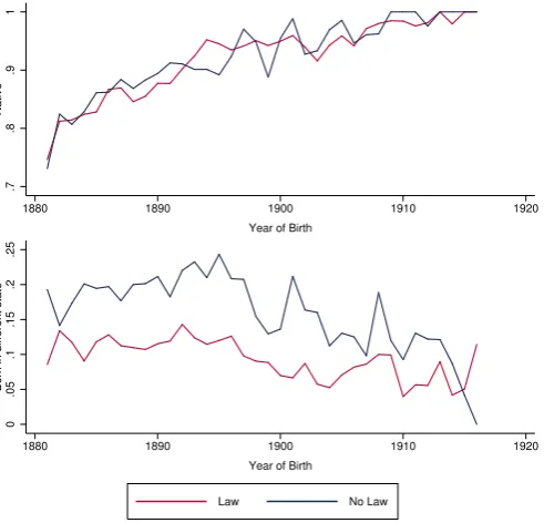
Figure 1.3 examines the balancedness of the linked data set in terms of the few available pre-treatment characteristics. The cross-border share of natives is comparable and does not vary systematically by cohort. The lower panel plots the share of “movers”, or individuals born in a state other than the state in which they are observed in 1920. Figure 1.3 shows that Michigan and Kentucky have a higher share of in-migration than do Indiana and Ohio. Although this phenomenon could be a worrisome indication of sorting across the border, in fact the trends move in

9_{For the 1940 census, Ancestry.com does not provide a digitized entry for parents’ birthplace.}

Recall that, for the 1940 IPUMS, only a random 5% of the sample were asked about parental birthplace.

10_{This is roughly comparable to the match rates of previous work linking individuals between}

(43)

[image:43.595.161.407.183.419.2]

parallel for the two groups of states over time; hence out-migration from states with a language law is not higher for the younger cohorts.

Figure 1.3: Balancedness of border data set

.7

.8

.9

1

Native

1880 1890 1900 1910 1920

Year of Birth

0

.05

.1

.15

.2

.25

Born in different state

1880 1890 1900 1910 1920

Year of Birth

Law No Law

Notes: The figure compares characteristics of the linked border data set across birth cohorts and across states with and without a language ban. The data consist of males, born 1880–1916 to German parents, who lived in a border county in 1920 and could be linked to the 1930 or 1940 census. The upper panel plots the share of native-born and the lower panel plots the share of “movers” (i.e., people who were born in a different state than the one in which they lived in 1920).

(44)

[image:44.595.113.524.138.378.2]

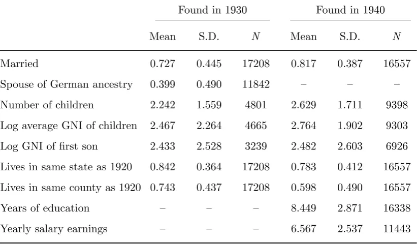
Table 1.2: Summary statistics: Border data set

Found in 1930 Found in 1940

Mean S.D. N Mean S.D. N

Married 0.727 0.445 17208 0.817 0.387 16557

Spouse of German ancestry 0.399 0.490 11842 – – –

Number of children 2.242 1.559 4801 2.629 1.711 9398

Log average GNI of children 2.467 2.264 4665 2.764 1.902 9303

Log GNI of first son 2.433 2.528 3239 2.482 2.603 6926

Lives in same state as 1920 0.842 0.364 17208 0.783 0.412 16557

Lives in same county as 1920 0.743 0.437 17208 0.598 0.490 16557

Years of education – – – 8.449 2.871 16338

Yearly salary earnings – – – 6.567 2.537 11443

Notes: The table shows summary statistics for males born 1880–1916 to German parents, who in 1920 lived in a county on either side of the border of Indiana (IN) and Ohio (OH) with Michigan (MI) or Kentucky (KY) and who were linked to the census of 1930 (left panel) or 1940 (right panel). See Section 1.5.2 for details on construction of the GNI variables.

Intermarriage. One key outcome of interest is intermarriage. It has been characterized as “the final stage of assimilation” (Gordon, 1964) and it is arguably a good indicator of immigrant integration in the host country, as it reflects accep-tance of the host culture on the part of the immigrans and vice versa. I investigate the extent to which being exposed to restrictive legislation at school affects the probability that second-generation German-Americans end up marrying within their own ethnic group.

(45)

predic-Figure 1.4: Locations of linked data set in 1920

Notes: The map shows the town-level location of all males, who were born 1880–1916 to German parents, living in a border county in 1920 and who could be linked to the 1930 or 1940 census.

tion. To the extent that the language of instruction in school affects the ethnic preferences of second-generation immigrants, we can expect to see changes in mar-riage choices later in life as one response to language restrictions. In particular, if removing German from the curriculum had the effect suggested by proponents of the policy, then English-only instruction should lead to greater assimilation as reflected in higher intermarriage rates. That might happen because, in the first place, children would no longer be indoctrinated “with the German language, cus-toms, and prejudices of the Fatherland. . .against the social and religious customs of the American communities in which they claim citizenship.”11 Greater familiar-ization with the American language and culture, as the Americanfamiliar-ization movement aimed to inculcate, would make these children prefer American spouses later in life. Second, to the extent that such Americanization would make these offspring more receptive to social environments other than their closed ethnic communities,

[image:45.595.91.449.105.391.2]

(46)

the market for marriage partners would contain more non-ethnic members and thus would increase the likelihood of intermarriage.

The earlier US censuses pose some difficulties for determining an individual’s ethnic background. In 1940, the question on parental birthplaces was posed to only 5% of the universe. This means that I can observe the ethnic background of the spouse of a native person only in 1930. In this census year, younger cohorts are observed at an age when they have likely not yet completed their marriage spells (ages 18–27). Comparison of these cohorts between states with and without a language law should still yield unbiased estimates, but they are not likely to be representative of the general population of German-Americans.12

First names. I use the names that individuals in my sample choose for their children as an additional proxy for ethnic identity. Names have an indisputable cultural component and to a great extent reflect the parents’ racial, ethnic, and social background and preferences (Lieberson, 2000; Fryer and Levitt, 2004; Head and Mayer, 2008; Cook et al., 2013). As such, the choice of first names for their offspring is indicative of parental tastes and, for immigrants, of assimilation into the host society. In particular, if cohorts affected by an anti-German law choose to give their offspring names that are less German-sounding and more common among natives, then that would indicate an assimilation effect of language restrictions.13

In order to measure a name’s ethnic content, I follow Fryer and Levitt (2004) in constructing an empirical index of German name distinctiveness, by using census data on first names and ethnic origin. This German name index (GNI), which captures how much more frequent a name is among the population of German origin compared with the rest of the population, is constructed as follows

GNIname,s =

Pr(name|Germans)

Pr(name|Germans) + Pr(name|non-Germans)

×100

12_{For example, Chiswick and Houseworth (2011) document a higher likelihood for endogamous}

marriages among individuals who marry young.

13_{Algan et al. (2013) show that the economic penalty associated with culturally distinctive}

names is an additional important determinant of parents’ naming decisions. In the current

(47)

[image:47.595.71.491.284.546.2]

A name found only among German ethnics would have index value 100, whereas a name given to no individuals of German origin would have index value 0. To compute this index, I use information from the 1930 5% IPUMS sample (Ruggles et al., 2010) and define Pr(German) as the share of foreign-born individuals in the census that were born in Germany. I compute this index separately for men and women and drop from the analysis all names that appear fewer than 10 times in the data; this procedure ensures that index values are not driven by rare names.

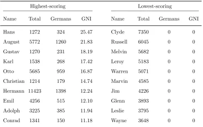
Table 1.3: Most and least German-sounding names in the 1930 census

Highest-scoring Lowest-scoring

Name Total Germans GNI Name Total Germans GNI

Hans 1272 324 25.47 Clyde 7350 0 0

August 5772 1260 21.83 Russell 6045 0 0

Gustav 1270 231 18.19 Melvin 5682 0 0

Karl 1538 268 17.42 Leroy 5183 0 0

Otto 5685 959 16.87 Warren 5071 0 0

Christian 1214 179 14.74 Marvin 4585 0 0

Hermann 11423 1398 12.24 Jim 4226 0 0

Emil 4256 515 12.10 Glenn 3893 0 0

Adolph 3225 385 11.94 Leslie 3795 0 0

Conrad 1341 150 11.18 Wayne 3648 0 0

Notes: The table shows the values of the German name index for the 10 highest-scoring (left panel) and 10 lowest-scoring (right panel) names of males in the 1930 5% IPUMS sample. Highest-scoring names are chosen among names that appear at least 1,000 times in the 1930 sample and are ordered by their GNI value; lowest-scoring names are ordered by popularity. See Section 1.5.2 for details on construction of the GNI.

(48)

but many of these names, including Hermann and Christian, are also on the list of most popular names among German immigrants. The right panel of Table 1.3 lists the 10 most popular names with a zero GNI value. Names such as Clyde, Russell, and Melvin are characteristically un-German in that they had been given to no German-born individuals in the 1930 IPUMS sample.14

In my data, the GNI is always highly correlated with gender and birth order. Males have a higher GNI than females, and the first-born son almost always has the highest value in the GNI among his siblings.15 _{In the main empirical analysis,}

I will use both the logarithm of the average GNI of all children and the logarithm of the GNI of the first son as outcome variables that proxy for ethnic identity.

1.5.3 World War II enlistment records

Data on men who enlisted in the US Army during World War II are from the Army Serial Number Electronic File, ca. 1938 –1946. The database is the end product of digitizing the original WWII draft computer punch cards by the Na-tional Archives and Records Administration. The complete database comprises of nearly 9 million records of enlistments in the Army, the Enlisted Reserve Corps, and the Women’s Army Auxiliary Corps. Each entry provides information on enlistment details (Army serial number, enlistment date and place, enlistment term and Army component), and also on several demographic and socioeconomic characteristics of the enlistee (nativity, race, civil status, birth year, birthplace, education, and occupation).

From this universe, I restrict my attention to a random sample of individuals born in Indiana, Ohio, Michigan, or Kentucky during the period 1880–1916. As with the IPUMS samples, I match the individuals to legislation based on their state of birth and thus limit the analysis to second-generation Germans. Be-cause the enlistment database does not contain information on the birthplace of an individual’s parents, I perform a procedure, similar to the one described in

14_{The GNI performs well in predicting an individual’s German ancestry among the second}

generation of Germans in the 1930 5% IPUMS sample; see Figure 1.11.

15_{Figure 1.12 shows that the GNI’s density for girls is to the left of that for boys. Figure 1.13}

(49)

Section 1.5.2, that links enlistees to the 1930 census and determines their ethnic origin, via Ancestry.com’s search engine. This is not the census year closest in time to the enlistment date range, but it is the closest one for which I can obtain information on parental nativity (since this variable is not usually recorded in the 1940 census).

Volunteers. Japan attacked Pearl Harbor in early December 1941. Only days later, Nazi Germany declared war to the United States. Following their country’s entry to World War II, thousands of American men volunteered for service. The decision to volunteer is motivated by patriotism and, in the case of first- or second-generation immigrants, it clearly signifies a strong identification with their host country. Especially for Germans, who would be called to fight against their country of origin, a decision to volunteer is an unmistakable indicator of assimilation.

It is not straightforward to determine whether a person volunteered for the Army or was conscripted. According to the draft classification, enlisted men are those members of the Armed Forces of the United States who volunteered for service. These individuals can be identified by their serial numbers, which belong to the 11 through 19 million series.16 _{However, it was possible for a drafted man}

to enlist in the regular army as a volunteer prior to his induction; doing so gave him more say in the choice of unit and conditions of service. This possibility introduces measurement error when serial numbers are used as a method to identify volunteers, yet the estimation procedure will not be biased provided this error does not differ systematically across cohorts and states. To reduce measurement error, I restrict my attention to men enlisted in 1942 — the year immediately following US entry into the war and during which enlisted men were most likely to be volunteers and not draftees.

Figure 1.14 plots the match rate between enlistment records and the 1930 census for the entire sample of men enlisted in 1942 and for volunteers.17 _Volatility

in the match rate is high, especially for older cohorts, but there are no systematic differences in the linking probabilities across states and cohorts. Table 1.4 gives summary statistics for the linked sample.

16_{Army Regulation no. 615-30, 1942.}

17_{The match rate is approximately 14%. Parman (2015) uses identical criteria to match a}

(50)

[image:50.595.113.523.137.317.2]

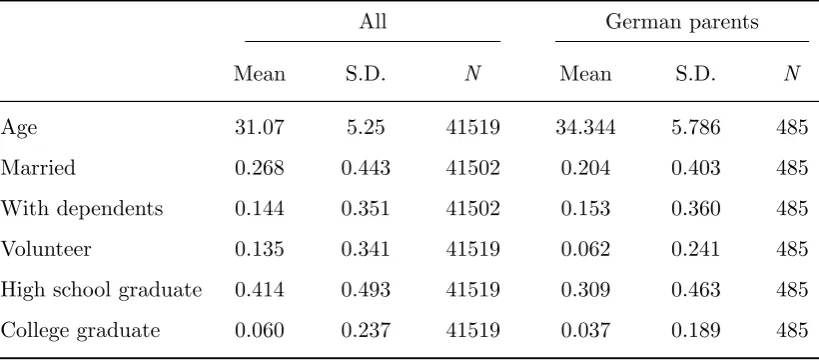
Table 1.4: Summary statistics: WWII enlistments

All German parents

Mean S.D. N Mean S.D. N

Age 31.07 5.25 41519 34.344 5.786 485

Married 0.268 0.443 41502 0.204 0.403 485

With dependents 0.144 0.351 41502 0.153 0.360 485

Volunteer 0.135 0.341 41519 0.062 0.241 485

High school graduate 0.414 0.493 41519 0.309 0.463 485

College graduate 0.060 0.237 41519 0.037 0.189 485

Notes: The table reports summary statistics for a random sample of males who enlisted in the US Army in 1942 and were linked to the 1930 census. The sample comprises of cohorts born 1880–1916 in Indiana, Ohio, Michigan, and Kentucky. The right panel restricts the sample to individuals with German parents. Volunteers are identified as having a serial number in the 11 through 19 million series.

1.6 Main results

My identification strategy is a difference-in-differences approach that is based on comparing cohorts of school age and cohorts too old to be at school between states with and without a language law. My main specification takes the form:

Yiscj =α+βTcsj+λc+θs+δZiscj+dsj+εisc (1.5)

whereTcsj is an indicator for individuals living in a state with a law and who were

within the age range for compulsory schooling at the time that law was in place. The termsλcand θs signify cohort and state of birth/residence fixed effects. dsj is

a fixed effect for the border segment (Michigan or Kentucky), andZiscj is a vector

(51)

allows for arbitrary patterns of autocorrelation within states across time but yields consistent estimates of the standard errors only with a sufficiently large number of clusters. To correct for the small number of clusters (n = 4) in my data, I always report p-values computed using the wild-t cluster bootstrap method of Cameron et al. (2008).18

In the above specification, state and cohort fixed effects account for average differences in the outcome variable across states and cohorts. As with every DiD approach, the identifying assumption is that there exists no omitted time-varying and state-specific factor correlated with the passage of language laws. The decision of states to adopt restrictive legislation was not entirely random; it was driven mainly by the share of the German element in the state’s population.19 _{To control}

for the potentially time-varying effect of this factor on outcomes such as endogamy rates, I always report specifications that interact the share of first- and second-generation Germans in a state in 1910 with cohort fixed effects.

Yiscj =α+βTcsj+λc+θs+δZiscj

+dsj +

37

X

c=1

γc×German shares×λc+εiscj (1.6)

It is worth remarking that there should be significant measurement error in my estimates because it is not known precisely which children of German origin attended schools where German was actually used as a language of instruction. This lack of sharp variation across cohorts in terms of the language of instruction will bias all estimates toward zero; yet it should not generate a systematic bias in the estimated coefficient of the difference in differences, which will be an average treatment effect on the entire population of Germans in relevant cohorts (including non compliers).

Threats to identification. The main DiD identifying assumption will be

18_{The significance of estimated coefficients in the entire analysis that follows is affected little}

when clustering at the state-cohort level or when adjusting for two-way clustering within state and within cohort (Cameron et al., 2011). Results available upon request.

19_{This can be verified by a mean comparison of the German share across states and also by a}

(52)

violated if legislation is endogenous to factors that directly affect assimilation out-comes. A plausible scenario is that Indiana and Ohio introduced restrictive laws because those states were characterized by relatively more anti-German sentiment. In that case there should be greater discrimination against Germans, which would affect some outcomes (such as intermarriage) directly and not through any mech-anism related to language used in school. This scenario is unlikely for three main reasons. First, in order for differences in the intensity of discrimination to have a differential effect on the younger cohorts exposed to school laws, these differences would have to be increasing over time. Yet we expect the opposite to be true because anti-Germanism peaked during and shortly after the war years and began to subside thereafter. In particular for endogamy, it is equally (if not more) likely that discrimination would affect marriage outcomes for the control cohorts born 1890–1900 — who would be at a marriageable age exactly during the war years — than the treated cohorts born after 1904. In any case, sources point to all states conducting a campaign of similar intensity against German during and after the war. Beck (1965) reports that both Ohio and Michigan had many proponents of a language ban, and language restrictions in both states faced militant opposition from Catholic and Lutheran churches. That German was banned in Ohio, but not Michigan, was due largely to idiosyncratic factors.

(53)

indicate no break around the treated cohorts. For my research design, this is an encouraging indication that parents did not relocate in response to language legislation.

A third and related concern is that of spillovers across the border. In particular, individuals living close to a state border — and who want to attend a German school — could always do so on the other side of the border, provided a school is close enough to their town. Therefore, restricting attention to border counties makes it easier to compare the treatment and control groups but also increases the possibility of measurement error caused by non compliers. The effect of spillovers would be to bias any estimated coefficients downward. In a robustness check, I will assess empirically the relevance of this concern by excluding from the data set all individuals who live very close to the border.

1.6.1 Intermarriage and first names

Panel A of Table 1.5 examines the average effect of legislation on the linked data set of males with German parents. Column [1] reports the estimated coefficient derived from a regression of equation (1.5)’s form. The estimate is negative, which suggests a decline in endogamy for treated cohorts. Column [2] inserts state con-trols measured pre-legislation in 1910 interacted with birth cohort dummies; hence this regression accounts for the effects of time-varying factors correlated with the law. These controls are, for year 1910, the share of first- and second- generation Germans and the sex ratio (computed as the ratio of males to females) among Germans in the state.20 _{The sex ratio is an important determinant of}

intermar-riage decisions (Angrist, 2002). During the period under study, the United States placed restrictions on immigration that could have distorted the ethnic composi-tion and sex ratios across states.21 Because immigration quotas were set on the basis of pre-existing immigrant shares, the included interactions partly control for this confounder by addressing the time-varying effect of population shares and sex

20_{I compute this using the 1% IPUMS sample for 1910.}

21_{The United States imposed a literacy test in 1917, seeking thereby to reduce immigrant flows}