Generic Neuromorphic Principles of Cognition and Attention for Ants, Humans and Real-world Artefacts: a Comparative Computational Approach

Generic neuromorphic principles of

cognition and attention for ants,

humans and real world artefacts:

a comparative computational approach.

Zenon Mathews

TESI DOCTORAL UPF / ANY 2010

DIRECTOR DE LA TESI

Paul F.M.J. Verschure

Acknowledgments

This doctoral thesis has been carried out at the Universitat Pompeu Fabra (UPF) in Barcelona, in the research group SPECS lead by Prof. Paul F.M.J. Verschure. My first and earnest thanks goes to Prof. Ver-schure, whose encouragement, supervision and constant support from the preliminary to the final level enabled me to develop and connect research ideas.

My deepest gratitude also to Dr. Sergi Berm´udez i Badia for the con-structive discussions, reviews and the abundant guidance over the many years that contributed crucially to my thesis. A semester project under the supervision of Sergi Berm´udez i Badia and Paul Verschure at the ETH in Z¨urich nearly five years ago started me on the path I traveled at UPF in Barcelona.

I would like to extend my special thanks to all SPECS members for the many useful feedbacks on my thesis and the great team work dur-ing several years. I have acquired invaluable scientific and social skills through the constant interaction with the SPECS group members.

I am heartily thankful to my parents and my brother for always being there when I needed them most, despite my negligence to visit them often enough. They deserve far more credit than I could ever offer.

Abstract

Resum

Summary

List of figures xxvi

List of tables xxvii

1 INTRODUCTION 1

1.1 The minimal components of biological cognition . . . . 2 1.2 Do biological cognitive systems use forward-models? . . 3 1.3 The stepwise refinement approach for modeling cognition 4 1.4 The cognitive system as a largely feedforward

mecha-nism: strengths and limits of an insect model . . . 5 1.5 Accommodating the forward-model for complex robotic

tasks . . . 6 1.6 Signature and model of anticipatory biases in human

vi-sual processing . . . 7

2 AN INSECT-BASED MODEL OF KNOWLEDGE

REPRE-SENTATION AND EXPLOITATION 9

2.1 Basic model and robot implementation for static environ-ments . . . 11 2.1.1 Experimental setup . . . 13 2.1.2 Task . . . 13 2.1.3 Simple model for mapless landmark navigation in

2.1.6 Heading direction accumulation . . . 18

2.1.7 Short and long term memories . . . 18

2.1.8 Results . . . 21

2.2 Extended model and comparison with the biological sys-tem in dynamic environments . . . 28

2.2.1 Navigational task and the test environment . . . 29

2.2.2 The extended model for mapless landmark navi-gation in dynamic environments . . . 32

2.2.3 Dynamic memory consolidation using expectations 34 2.2.4 Results . . . 40

2.3 On the necessity of top-down cognitive influence on per-ception . . . 47

3 PASAR: AN INTEGRATED BOTTOM-UP AND TOP-DOWN MODEL FOR ACTING IN DYNAMIC UNCERTAIN ENVI-RONMENTS 49 3.1 Related Work . . . 51

3.2 Research Question . . . 52

3.3 The model and the components . . . 53

3.3.1 World Model . . . 55

3.3.2 Prediction, Anticipation and Sensation . . . 55

3.3.3 Top-Down and Bottom-Up Attention . . . 59

3.3.4 Sensory Data Alignment . . . 60

3.3.5 Motor Response . . . 62

4 TESTING PASAR: CONTROLLING ARTEFACTS IN REAL-WORLD DYNAMIC ENVIRONMENTS 65 4.1 eXperience Induction Machine (XIM) . . . 66

4.2 Rescue Robot Simulation . . . 66

4.3 Data Collection . . . 68

4.3.1 XIM . . . 69

4.3.2 Rescue Robot Simulation . . . 70

4.4 Data Analysis . . . 72

4.5.1 Mixed Reality Space XIM Testbed . . . 72

4.5.2 Robot Rescue Simulation Testbed . . . 80

4.6 Conclusions . . . 82

4.7 Discussion . . . 83

5 TESTING PASAR: THE BOTTOM-UP AND TOP-DOWN INFLUENCES IN HUMAN VISUAL PROCESSING 85 5.1 Methods . . . 87

5.1.1 Model . . . 87

5.1.2 Displacement detection task . . . 92

5.1.3 Psychophysical reverse correlation . . . 94

5.2 Results . . . 96

5.3 Conclusions . . . 99

6 CONCLUSIONS 101 7 APPENDIX 107 7.1 MCMC Implementation for JPDA Event Probability Com-putation . . . 107

7.2 Sensory MAP Alignment Learning in the XIM Mixed-Reality Space . . . 108

7.3 Multi-robot Testbed Equations . . . 111

7.4 Multi-Person Tracking Experiment in XIM . . . 113

List of Figures

2.1 (A) The artificial forager SyntheticAnt. The robot is

2.2 Contextual learning of landmarks:(A)Activation of HDA cells as a sinusoidal function of the angular difference from the cell’s preferred angle. (B) HDA-set activation for a group of 36 HDA cells (of 10◦resolution each) for a movement indicated by the arrow. Blue and red lines rep-resent positive and negative activations respectively. (C)

An example of a foraging run from nest to feeder travers-ing some landmarks indicated by the colored shapes. (D)

2.4 Foraging to landmark navigation: All plots are super-imposed on the tracking camera image. The vertical bar in the middle of the image belongs to the wooden struc-ture of the wind tunnel and does not interfere with the movement freedom of SyntheticAnt. (A) Foraging and

homing. The red dots indicate robot positions during

for-aging from nest to feeder. The green circles indicate en-countered landmarks. The white arrows indicate the cor-responding HDA sets from the DAC contextual layer. The blue square on the right is the feeder. The yellow arrow corresponds to the computed homing HDA. The yellow track shows the homing behavior of the robot after feeder detection. (B) Nest to feeder trajectories. SyntheticAnt

is guided through two different trajectories from nest to feeder (indicated as run 1 and run 2, leading through avail-able landmarks. (C) Generalization of homing. Af-ter the runs shown in B, SyntheticAnt is kidnapped and placed in an arbitrary position in the arena. Upon land-mark detection SyntheticAnt recalls all possible straight routes to other landmarks including the nest and feeder, indicated by the white arrows. (D) Route execution. Af-ter recall,SyntheticAnttraverses recalled routes. . . 22

2.5 Foraging behavior as density plot: Position data from

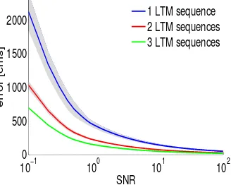
2.6 Bayesian merging of LTM sequences:The error in hom-ing vector computation (or in landmark to landmark route recall in general) as a function of the SNR of the HDA computation. The errors when using one, two or three LTM sequences in combination are shown. The colored lines are mean values and the patches signify standard de-viation. . . 27

2.7 Acting in a dynamic world: SyntheticAntwas exposed

to virtual obstacles (filled circle) placed on its route dur-ing homdur-ing or landmark navigation. The tracked posi-tions of the robot are indicated by the yellow dots. . . 27

2.8 Insect behavioral analysis, modeling and testing on robots:

A)Real-world ant experimental studies are performed and the behavior of the ant is recorded using a tracking cam-era. Controlled manipulations of visual landmarks in the ant arena are made in order to analyze the ant behavior.B)

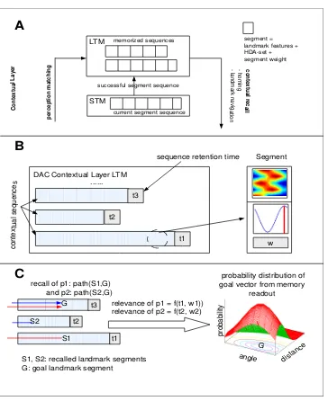
2.10 (A) DAC Contextual LayerA segment contains the ex-tracted landmark features, an HDA-set and the segment weight. Segments are sequenced temporarily in the short-term memory (STM) whenever a landmark is encoun-tered. Upon feeder detection, the contents of the STM are transferred into the long-term-memory (LTM). Dur-ing recall phase (homDur-ing, landmark navigation), the LTM is matched against the current sensory events and an opti-mal trajectory is computed from recalled LTM segments.

(B) Sequencing: During the foraging runs from the nest

to the feeder, encountered landmarks are chained in the DAC contextual layer short-term memory (STM) together with the HDA set. Each LTM sequence has a retention time towing to the transiency of memory and each seg-ment has a weightw. (C) Recall:During the recall phase, the HDA-sets starting from the recalled segment to the goal segment are combined to compute the optimal hom-ing vector. When the recalled segment and the goal seg-ment are on different LTM sequences, the segseg-ments from the recalled segment to the nest on one sequence, and the nest to the goal segment on the other are combined (such a combination is calledpath). Pathsare weighted accord-ing to the retention time of the sequence and the mean relevance weights of the segments of the recalled LTM sequence. . . 33

2.11 Dynamic Memory Reconsolidation Schema:As a

2.12 Expectation reinforcement for memory consolidation:

Discrepancy between expected paths and computed paths are used to consolidate memory by means of setting LTM segment weights and writing new LTM sequences. . . . 39

2.13 Expectation reinforcement for learning stable landmarks:

A) Before the test runs (but after several foraging runs)

SyntheticAnt has encountered all 10 landmarks, but has the same confidence in all of them. The observed vari-ance is due to different LTM sequence acquisition times.

B)After 5 test runs, during which 9 out of 10 landmarks were displaced, the probability distribution for the con-fidence changes. C)The confidence probability distribu-tion after 10 test runs. The plot shows the computed home distances and angles (as a probability distribution) using individual landmarks using memory recall for each land-mark. The indicated skewness values are the third central moments of sample values, divided by the cube of their standard deviations. The growing skewness from left to right indicates growing asymmetry in the distribution. . . 42

2.14 Confidence recovery and search intensities: The

re-covery of confidence with time (after initialization of the L´evy search) is indicated. High intensity searches (indi-cated by theθ values) reach a certain confidence thresh-old quicker. A high intensity L´evy search is initialized when a landmark is missing and a low intensity one is launched when a low confidence landmark is encountered

2.15 Real ant benchmark: The upper panel and lower pan-els show real and Synthetic ant data in the same land-mark manipulation task. The ant performs 25 foraging runs from nest (located at the right end the arena) to the feeder (at the left end of the arena). The arena contains displaceable visual landmarks and also non-displaceable obstacles, both of which the ant cannot walk over. Trajec-tories are indicated by white lines. The density maps are computed from the trajectories; we define here density as inversely proportional to theconfidencein the landmarks.

A)Ant trajectory in the 21st foraging run. B)Ant trajec-tory in the 22nd run, where some landmarks were manip-ulated at the indicated positions. C) In the next run (23) all the visual landmarks are again placed in the positions as in runs 1 to 21. D)The density plot of trajectory after landmark restoration. The lower panel shows the perfor-mance of theSyntheticAntin the same experiment. E) Be-fore the manipulation, theSyntheticAnthas the same high confidence value in all landmarks and therefore does the traversal on almost a straight line. F)Upon manipulation, a high intensity L´evy search is initiated and propagated back home. G) Upon restoration, a low intensity search at the low confidence landmark is performed, as captured by the density plot.H)The confidence in the manipulated landmark recovers slowly as indicated by the density plot. 45

2.16 Position density norms reflecting task resolution times:

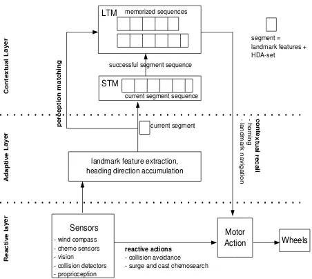
3.1 PASARproposes a three-layered distributed architecture: reactive, adaptive and contextual (as in [113]). The reac-tive layer contains the physical sensors and the feature extraction mechanisms. The adaptive layer contains the

data alignment, the data association and saliency com-putation mechanisms. The contextual layer contains the

world-modeland thegoalsof the system. The arrows in-dicate information flow, and the colored arrows inin-dicate sensation and bottom-up attention (red), prediction and anticipation (blue) and top-down attention (green). The

motor responseis a result of the integration of the bottom-up and top-down saliency maps. . . 54 3.2 Schematic of world-modeland selective attention

gener-ation for a dynamic scenario. Left panel: A dynamic scene as perceived by an autonomous system. Four en-circled objects are perceived as closed entities by the au-tonomous system. Middle Panel: Fourconcepts (mem-ory representation of real-world objects) inn = 3feature space with hue, weight and height as example features. The ellipsoids represent the covariance of the concepts.

Right Panel: The top-down attention mechanism

initi-ates an action that might have an immediate effect on the world model (arrow 3) as the sensory input is changed by the performed action. . . 56

3.3 Saliency computation from multimodal sensory input:

The multimodal sensory input(A) is associated to exist-ing targets by means of the anticipatory fields of JPDA

(B). The top-down biasing of the anticipatory fields using the world-model is applied before data association. The bottom-up and top-down saliency maps are combined us-ing a common neural group onto which both the above saliencies are mapped(C). A winner-take-all WTA neu-ral network computes a single winner from this map(D)

4.1 The eXperience Induction Machine (XIM)can be con-sidered as an artificial organism in the shape of an en-vironment, that has its own goals and expresses its own internal states. It comprises a pressure sensitive floor, overhead and pan-tilt cameras (gazers), movable lights (light-fingers), triplets of microphones for sound recogni-tion and localizarecogni-tion, projecrecogni-tion screens and ambient and directional sound output (adapted from [70]). . . 67

4.2 XIM Multiuser Interaction Scenario:Multiple real users

interacting with each other in a mixed reality Pong game, which is one of the scenarios used to evaluated PASAR performance. Also remote users take part in the same interaction by logging in from remote machines into the virtual world and they are represented by avatars on the projection screens (adapted from [55]). . . 68

4.3 PASAR multi-robot rescue scenario. LeftSnapshot from

PASAR Experiment: The bigger circle surrounding PASAR shows sensory range. Everything outside this range is not perceived by PASAR. The smaller circles surrounding some of the agents indicate that the corresponding agents are expired. The base station, where PASAR recharges itself, is indicated by the rectangle on the left bottom.

RightExample of the predicted total utility as a

4.4 Sensory Map Learning Using PASAR Adaptive Layer: Ashows the error map in [cms] for the overhead infrared camera tracking before learning (mean 75 cms). High er-rors are due to camera perspective and distortive erer-rors.B

shows the error after online learning with a single user in XIM (mean 26 cms). CThe validation gates of the con-cepts(i.e. the tracked persons) for the tactile floor modal-ity are made larger along the periphery of the space. Us-ing this top-down bias in PASAR improves the trackUs-ing error significantly (mean 14 cms). The error distributions decrease significantly fromA to B toC (Tukey-Cramer multiple comparison,p <0.05) . . . 73

4.5 PASAR for multimodal multitarget tracking: Ashows

correctness of ID resolution in cluttered situations of track-ing with 2 to 5 persons freely interacttrack-ing in XIM.Bshows ID resolution accuracy for different interaction scenarios (see text for further details). . . 74

4.6 PASAR for multimodal multitarget tracking: ID

reso-lution performance percentage as a function of the num-ber of objects tracked in XIM simulation. . . 75

4.7 Usage of a priori knowledge: spatiotemporal

congru-ence of multimodal data in XIM Multimodal data that

is proximal to data of another modality in space and time has an added weight. The scenario numbers 1,2,3,4 refer to the interaction scenariosexploration, energy, center of mass, pong gamerespectively. . . 76

4.8 Usage of a priori knowledge: spatiotemporal

congru-ence of multimodal data in simulation: The accuracy of

4.9 Attention-guided feature extraction under noise and

limited resources constraints: PASAR attention system

follows subjects in XIM and hue extraction from torsos. Two such attempts are shown, one for green and one red. The snapshots are from a moving camera image and the bottom indicates the images used for hue extraction. The Region-of-Interests (ROIs) of the images used to extract the hues are indicated by the white rectangular boxes in the smaller images at the bottom. . . 78

4.10 Attention-guided feature extraction under noise and

limited resources constraints: A)Subjects with two

dif-ferent hues are identified as belonging to two difdif-ferent hue bins with a significant difference (student’s t-test, p

< 0.05). B) Latency of recuperation: Latency of

re-cuperation of IDs using hue feature extraction after an ID confusion (mean 17 seconds). The data shown is ex-tracted from two subjects acting simultaneously in XIM for 5 minutes. . . 79

4.11 Total expiry time of robots as a function of the

mem-ory decay: Memory decay rate is used in seconds.

De-cay rate refers to the time in seconds in which theconcept

variance falls to a predefined baseline. . . 80

4.12 Total expiry time for different testcases: Performance

5.1 Schema of ellipsoidal anticipatory gates: A: Moving targets with predicted positions indicated by arrows. B:

Ellipsoidal anticipatory gates for data association.C: Tar-get states after one movement step. One anticipation was violated by a displacement (bottom right) and the dis-placement falls outside the anticipatory gate. The ques-tion mark indicates if the subjects answers ”yes” or ”no” to the question if this displacement was noticed. . . 92

5.2 Schematic of the psychophysical kernel computation:

All trials are sorted to detected and non-detected trials and all displacements normalized. A single kernel is com-puted from the density plots of the two sorted data groups (see text for more details). . . 94

5.3 Psychophysical kernelsfor all subjects for conscious

de-cision, early and late saccades and in different cognitive loads (low, medium and high). The area (a), eccentricity () and the orientation (γ) of the kernel ellipses are indi-cated. . . 97 5.4 a) Saccade histograms with early and late saccade

inter-vals indicated. b)Change in intra-subject eccentricities.

c)Change in intra-subject orientations. . . 98

7.1 Learning Sensory Maps: Using the PASAR adaptive

layer, the space representation errors of one sensory modal-ity are corrected using a different modalmodal-ity stimulus. . . 109

7.2 Online learning of the extrinsic parameters of

mov-able cameras:Using the PASAR adaptive layer, the

List of Tables

2.1 Neural simulation parameters . . . 23

2.2 Landmark stability learning experiment:the table shows

the ten landmarks available in memory, the angle and dis-tance from each landmark to feeder, the segment rele-vance of the segment containing the landmark (rseg) and the retention time (tret_{) of the memory sequence from}

which this landmark recalled. . . 41

5.1 p-valuesof the two-sided sign test for the eccentricity()

and orientation(γ) differences of the psychophysical

ker-nel ellipses at individual subject level between low(l), medium(m) and high(h) load experiments. The kernels computed by

the subjects’ decisions, the express saccades and thelate

Chapter 1

INTRODUCTION

More than a decade ago, Allen Newell argued that a model of a cogni-tive system should be capable of explaining how intelligent organisms flexibly react to stimuli from the environment, how they predict future events, how they exhibit goal-directed rational behavior, how they repre-sent knowledge, and how they learn [81]. Newell also defines the term cognition to include perception and motor control. Despite intense re-search in cognitive sciences, it still remains unclear how these specific mechanisms such as prediction, anticipation, sensation, attention, mem-ory or behavior contribute to the general process of cognition and how they interplay in autonomous systems acting in dynamic uncertain en-vironments [129]. On the one hand this question has been the starting point for several behavioral and neuroscientific studies, with the goal of understanding the biological brain. On the other hand, this question has also been of immense interest to roboticists building artificial cognitive systems acting in real-world environments. This is because evensimpler

that of traditional artificial intelligence point of view. We model the min-imal components of cognition, aiming to capture the key ingredients of cognition and their interplay.

1.1

The minimal components of biological

cog-nition

We first address the question of what minimal set of mechanisms are necessary for a cognitive system. Unveiling these minimal components serves as the starting point of our investigation about the interplay among them. One such mechanism, namely the one that predicts the future state of a system given the current state and the control signals, is increasingly thought to play an important role in neuroscientific explanations of motor control, goal oriented behavior and cognition [128]. The existence of such a mechanism, known conventionally as theforward model, means that bi-ological systems should be able to predict the sensory consequences of their actions in order to have robust adaptive behavior. In this context, the distinction between vertebrate and invertebrate nervous systems be-comes crucial as the cognitive capabilities of animals from the two ani-mal groups largely vary. In vertebrate neuroscience, there is substantial interest in interpreting the function of various brain areas in these terms (e.g. the cerebellum [76]). Besides, several authors have suggested that forward modeling could be a unifying framework for understanding the brain circuitry that underlies cognition [27, 11, 31]. The components of a forward model not only include sensory input, sensory processing, motor command and motor output, but also a prediction mechanism of future stimuli [120, 60]. In this context, the notions oftop-downandbottom-up

bottom-up dialogue with lower areas (midbrain and sbottom-uperior colliculus) to solve low-level tasks like multisensory integration [101]. In the context of this dissertation we take a phylogenic approach to model a modular cogni-tive system, starting with a simple model and then incorporating forward models to account for observed insect navigational behavior in dynamic scenarios. We then generalize and test our model in complex real-world and simulated robotic tasks and in human visual processing.

1.2

Do biological cognitive systems use

forward-models?

is not evident that the invertebrate kingdom does not posses such capabili-ties, e.g. insects have brain structures called the mushroom bodies, which might have comparable functions [53]. Evolution is yet another argument that speaks for unique higher cognitive capabilities in higher animals, as adapting to more complex habitats should have given rise to more com-plex cognitive capabilities [36]. At the anatomical level, the difference in cognitive capabilities is remarkable, materialized in the number of neu-rons and synapses and in the complexity of brain layer structuring [106]. In summary, there is a general consensus that higher animals like mam-mals use forward mechanisms like prediction or anticipation to achieve adaptive behavior in uncertain environments. Nevertheless, the question whether invertebrates do the same or if their task solving behavior can be explained with relatively simpler models, without explicit use of forward models, is still subject of debate.

1.3

The stepwise refinement approach for

mod-eling cognition

We follow the principle of stepwise refinement in modeling the key cog-nitive components. We start with the relatively simpler nervous system of the ant and investigate the behavior of the ant in navigation tasks and we finish with a model that integrates prediction, anticipation, sensation, attention and motor response.

1.4

The cognitive system as a largely

feedfor-ward mechanism: strengths and limits of

an insect model

1.5

Accommodating the forward-model for

com-plex robotic tasks

We update our model to accommodate higher-level cognitive mechanisms like prediction, anticipation and attention and test the refined model for solving complex robotic tasks. Our model is inspired by the immense efforts invested over the past two decades in discovering the brain mech-anisms involved in the interplay between prediction, anticipation, percep-tion, memory and action [66]. Scrutinizing the highly hierarchichal struc-ture of the brain has been a starting point for various studies investigating these subcomponents of cognition. The interdisciplinary research of cog-nitive brain and robotics research has profited from the above findings about the key hierarchical and vertical mechanisms involved in biological cognition.

con-textual [113]. In our simulation and real-world robotic experiments, we address the question of how each sub-component of PASAR contributes to the overall performance in the given task and what insights we can gain about robotic control and cognitive mechanisms in general. By perform-ing these experiments we want to gain deeper insights into the interplay of the different cognitive subsystems involved in solving complex tasks. In order to test the hypothesis posed by our model about the specific inter-play of attention, prediction and anticipation, we perform a psychophys-ical experiment with humans, thereby validating the model in biologpsychophys-ical cognition.

1.6

Signature and model of anticipatory biases

in human visual processing

Chapter 2

AN INSECT-BASED MODEL

OF KNOWLEDGE

REPRESENTATION AND

EXPLOITATION

land-mark navigation as a benchland-mark task to understand the basic cognitive principles employed by ants.

Ants have been investigated widely for their remarkable navigational capabilites. Ants, like a wide range of other animals, are foragers and robust navigation skills are crucial to survival for foraging successfully in unknown environments [103, 122, 127, 29]. Some remarkable behaviors such as landmark navigation, homing, path integration (PI) and learning are in many occasions required to perform successful foraging. Many ant species, like the desert ant (Cataglyphis Fortis), are known to forage successfully in very dynamic environments and find their way back to the nest, speaking for their robust navigational skills in changing envi-ronmental conditions. Also, ants are a particularly interesting preparation since the navigation of ants in dynamic environments can be tested in a controlled manner in indoor ant arenas. We design a minimal cogni-tive model that can capture ant behavior and implement it in a real-world robotic platform to navigate using the same model.

2.1

Basic model and robot implementation for

static environments

Our initial navigational model is inspired by the discussion about the pres-ence or abspres-ence of a cognitive map in the insect brain. The concept of

cognitive map for navigation, carried out mainly by Tolman [105], was fuelled by the discovery of the so-called place cells in the hippocampus of the rat and has widely increased our understanding of cognitive navigation mechanisms [84, 85]. It spawned early research on navigational strategies in cognitive neuroscience based on hippocampal representations of space [86, 22, 77]. While mammals are assumed to learn a place/map-like rep-resentation for foraging [84, 85], this does not seem the case in insects.

Insect navigation has been studied for more than a century [117, 28, 122, 98]. Interestingly, a wide range of findings suggests that insects do not rely on a map for solving foraging tasks [123, 28]. Recent studies suggest that rather than using map-like representations, insects make opti-mal use of proprioception, landmark recognition and memory to navigate [29]. In particular, desert ants use sun position and visual panorama for heading direction computation [122, 4]. Complex allocentric navigational behaviors using mainly ego-centric cues can be seen both in mammals like rodents but also in insects like ants and bees, which have consider-ably lower computational resources with only hundreds of thousands of neurons. Therefore, insect navigation studies are useful in that they reveal essential components for an efficient mapless navigation strategy. This is especially relevant for robotic implementations of autonomous systems and artificial foragers.

fa-miliar environments like mazes and small enclosures [64]. Navigators using such map based models of navigation are required to learn those place representations [50, 131]. Moreover, only a few of those models have been tested with real robots [46, 45].

As map based navigation strategies suffered from an inability to tra-verse unvisited regions of space, newer theories have incorporated path integration and head direction signals [107]. Even more recent versions also include cortical grid cells but still concentrate on the self-localization aspect of navigation rather than navigation between places [51, 75]. At the same time, the parsimonious navigation strategies of insects offer a guideline for computationally cheaper and eventually simpler navigation methods for mobile robots. A number of models exploit and reproduce some of the capabilities required during foraging [15, 16, 93]. However, many are biologically unrealistic and only deal with a very limited forag-ing task.

This section describes a comprehensive mapless biologically based model, including chemical search, PI and landmark navigation, of in-sect navigation strategies that is implemented in the framework of the Distributed Adaptive Control (DAC) architecture [113, 111]. The orga-nization of behavior and optimal use of landmark recognition, proprio-ceptive information, heading direction information and memory usage is controlled by DAC and tested on an artificial foraging ant robot. Our results show a successful integration of a number of biologically based models and behaviors that give rise to realistic foraging. Moreover, our model explains the generalization process as a probabilistic use of mem-ory, which generates allothetic behavior from a limited set of idiothetic cues in static environments.

heading direction accumulators. After foraging, landmark navigation is tested with the odor source turned off. Our results show stability against robot kidnappingand generalization of homing behavior to stable map-less landmark navigation. This demonstrates that allocentric and efficient goal-oriented navigation strategies can be generated by relying on purely local information. Furthermore, we argue that ant brain does not need to possess any forward model to achieve stable landmark navigation in static environments. Consistent with recent findings the model supports navigation using heading direction information, thus precluding the use of global information [123, 124].

2.1.1

Experimental setup

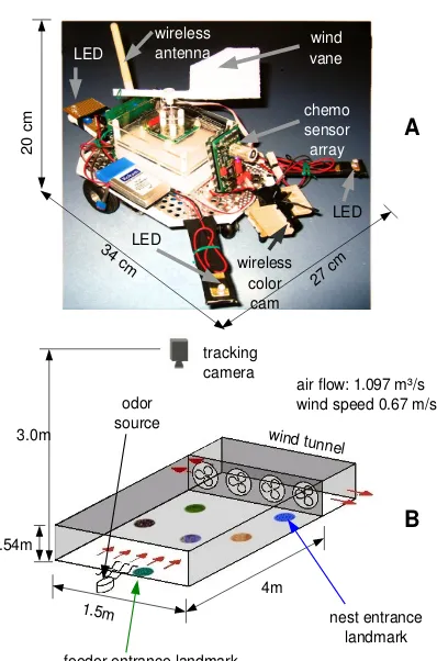
The experimental scenario consists of a robot forager calledSyntheticAnt, which is tested in a controlled indoor environment (figure 2.1). The test environment consists of a wind tunnel used by SyntheticAnt to localize the feeder tracking an odor plume. The wind tunnel floor contains a set of visual cues (landmarks) forSyntheticAnt to learn its way through the environment. A vision based overhead tracking system (AnTS) is used to localize the robot and compute its heading direction within the test arena, allowing for an analysis of the behavior of the robot.

2.1.2

Task

tracking  camera

1.5m 4m

wind tunnel

nest entrance landmark feeder entrance landmark

0.54m 3.0m

odor  source

air flow: 1.097 m³/s wind speed 0.67 m/s

wind vane

chemo sensor array

wireless color  cam

wireless  antenna

LED

LED

LED

34 cm

27 cm

20 cm A

B

Figure 2.1: (A) The artificial forager SyntheticAnt. The robot is equipped with a wireless color camera for visual cue recognition, a chemosensor array for odor detection, a wind sensor for wind direction computation and three LEDs for head direction computation using an overhead tracking system. The camera image is transmitted using a 2.4 GHz analogue wireless link. The exchange of motor commands and sen-sor readings with the robot are realized via a serial port over Bluetooth.

(B) Wind tunnel arena. At the back of the wind tunnel there are exhaust

placing the robot in an arbitrary location in the absence of the odor plume. Hence, in order to achieve this,SyntheticAnthas to recall the memorized landmarks and be able to navigate to other landmarks, including the nest and the feeder.

In figure 2.2A), each HD accumulator cell stores the value d×cosθ

wheredis the distance indicated by the movement arrow andθ the devi-ation angle of the movement from the preferred angle of the accumulator cell. The slope of activation falls as a sinusoidal function of angular devia-tion from the actuated direcdevia-tion, being 0 at 90◦. In figure 2.2C), Individual paths from landmark to landmark are indicated by numbers 1..4. In fig-ure 2.2E), after several foraging runs, the LTM contains several segment sequences (a segment is defined as a combined representation contain-ing the landmark features of one landmark and a HDA set) of different lengths since in each foraging run only a subset of available landmarks are visited. In figure 2.2C), Note that the recalled segment and the goal segment can be on different LTM sequences, in which case the segments from the current landmark to the nest on one sequence, and the nest to the goal landmark on the other have to be combined.

2.1.3

Simple model for mapless landmark navigation in

static environments

H D A  c e ll  a c ti v a ti o n :  c o s (  

deviation  from preferred angle 1 0 ­1 180˚ ­180˚   0˚ A B   0˚    180˚   90˚  270˚ nest C feeder 1 2 3 4 D 33 HDA cells [1..36] c e ll  a c ti v a ti o n ­0.2 0.2 1 ­0.23 0.23 ­0.34 0.34 3 0.29 ­0.29 32 4 2 3 10 ... ... DAC Contextual Layer LTM c o n te x tu a

l se

q u e n c e s Segment la n d m a rk   fe a tu re s H D A  s e t DAC Contextual Layer STM ... upon feeder  detection recalled

landmark landmarkgoal

LTM sequence + .... HDA set E F

behavior, and have been shown to be compatible with formal Bayesian models of decision making [112]. All computations are implemented us-ing the neural simulation tool IQR [17].

2.1.4

Reactive behaviors

The reactive layer ofSyntheticAntimplements a set of reactive behaviors including:

• Chemical search: SyntheticAnt implements a model based on the best studied case of chemotactic behavior, moth chemotaxis (as in [93]). It consists of an upwind movement (surge) whenever the animal perceives the odor stimulus and otherwise an oscillatory crosswind search (cast) un-til the odor plume is found again. The implementation of this behavior was done using the IQR neural simulator [17].

•Collision avoidance: Virtual proximity sensors, derived from the track-ing system (figure 2.1), are used to avoid immediate collisions.

• Feeder detection: After finding the feeder (odor source)SyntheticAnt

returns to the nest using a computed home vector by means of path inte-gration, further referred to ashoming.

In the absence of the odor plume SyntheticAnt’s surge-and-cast reactive behavior simplifies to a simple cast, which enables SyntheticAnt to ex-plore the environment until a memorized landmark is encountered. In the absence of the odor plume a stochastic behavior is employed to avoid getting stuck.

2.1.5

Landmark recognition

2.1.6

Heading direction accumulation

Path integration (PI) uses self-motion cues to compute the vector between the navigator’s current position and the starting point, i.e. home base. In our model we make use of heading direction and proprioceptive infor-mation to acquire PI. We propose the use of head direction accumulators (HDA), as postulated in [64]. A HDA is a neuron that fires only when the navigator heads in a particular direction. Furthermore, the firing rate of such a neuron correlates with the distance covered in that direction (fig-ure 2.2, B). HDAs are assumed to integrate sensory information such as optic flow, polarized photoreceptors, sun position and proprioceptive in-formation until reset [64]. Hence, a group of HDA neurons each of which is tuned to a different angle at equal intervals covering 0 to 360 degrees encodes the direction and distance from the previous position at which the HDA-set was reset. The activation of an HDA-set is governed by a cosine function as shown in figure 2.2. The slope of the activation rate is highest when the navigator moves in the HDA cell’s preferred direction and falls according to the cosine function with angular deviation, consis-tent with [64] [100]. During foraging, wheneverSyntheticAntencounters a landmark, the set of detected landmark features and the current HDA information is passed to the STM of the contextual layer of DAC, as dis-cussed in the next subsection. After that, the HDA-set is reset and the foraging continues.

2.1.7

Short and long term memories

landmark feature extraction, heading direction accumulation Motor Action A d ap ti ve  L ay er R ea ct iv e  la ye r C o n te xt u al  L ay er Sensors ­ wind compass ­ chemo sensors ­ vision ­ collision detectors ­ proprioception Wheels p er ce p ti o n  m at ch in g LTM STM successful segment sequence current segment segment =  landmark features +  HDA­set current segment sequence memorized sequences reactive actions ­ collision avoidance ­ surge and cast chemosearch co n te xt u al  re ca ll ­ h om in g ­ la nd m ar k  na vig ati on

against the current sensory events. Goal cue is defined as a the feature set characterizing a specific landmark. Matching LTM sequences containing both current sensory perception and goal cues are recalled to compute the optimal route from the current position to the goal landmark. Matching is accomplished by the following distance function:

d(a, b) = 1

K

X

i

| ai

max(a) −

bi

max(b)| (2.1)

a whereaandbare vectors in_RK _{andais the current activity of the cue}

information and b is the stored cue information. A segment is selected when the distance1−d(a, b)is higher than a predefined threshold. The selected segment and segments stored in the same sequence together con-tain the accumulated PI information (HDA) to the goal.

To compute the optimal route from the currently perceived landmark to an arbitrary landmark, we consider the scenario where the currently selected segment (landmark) and the goal segment (landmark) are on dif-ferent LTM sequences. To do this, we first compute the homing vector by summing and inverting the sequence of HDA-sets stored in all segments from the currently selected segment until nest on the first sequence. To this we add the sum of the HDA-s from nest to the goal segment (land-mark) on the second sequence. This allows computing optimal routes be-tween any two landmarks represented in arbitrary segments in the whole LTM.

After multiple foraging runs,SyntheticAntmight encounter landmarks, that had been seen in different foraging runs. This fact will select seg-ments of different sequences in the LTM during recall. In this case, each selected segment will return a homing vector, which have to be merged optimally. This generalizes from homing to landmark navigation if the goal landmark is not the nest. In general we refer to the decoded heading direction and distance as action(or action HDA-set). Assuming a white noise error, this decoded heading direction and distance to the goal can be formulated as a 2D Gaussian probability distribution:

¯

where X¯ = [α, δ]T_{. α is the angle and δ the distance coded by the}

ac-tion HDA-set. The acac-tion HDA-set, X¯, can be formulated as a Gaus-sian distribution with mean µ¯ and variance σ2_{. The variance σ}2 _grows

with the total distance dist covered during the heading direction accu-mulation. This can generally formulated as a function: σ2 = f(dist). Given this Gaussian distribution for each recalled segment action, we use Bayesian inference to compute the best action. If n actions are recalled, the best action a is the action with the highest conditional probability:

P(a|X¯1,X¯2, ...,X¯n). And using Bayes theorem., the probability of the

optimal action is computed:

P(a|X¯1,X¯2, ...,X¯n) =

P(a)P( ¯X1,X¯2, ...,X¯n|a) P( ¯X1,X¯2, ...,X¯n)

(2.3)

where the numeratorP(a)P( ¯X1,X¯2, ...,X¯n|a)is the joint distribution

P(a,X¯1,X¯2, ...,X¯n)and the denominatorP( ¯X1,X¯2, ...,X¯n)is a constant

without effect.

Using conditional independence of memory sequences, the above equa-tion can be reformulated as:

P(a|X¯1,X¯2, ...,X¯n)∝P(a)

n

Y

i

P( ¯Xi|a) (2.4)

P(a) is uniformly distributed in an a priori unknown environment. Therefore, the computation of P(a) in equation 2.4 can be reduced to the product of Gaussians X¯1,X¯2, ...,X¯n. The resulting action with the

highest probability is optimal in the Bayesian sense.

SyntheticAntruns on an Intel(R) Core(TM)2 Duo CPU 2.66GHz ma-chine with GNU/Linux Suse10.3 operating system at about 35 Hz. The parameters of the neural simulation using the IQR toolkit [17] is summa-rized in table 2.1.

2.1.8

Results

D B

C A

run

1

run 2 nest

nest

feeder

feeder

SyntheticAnt

position

Figure 2.4: Foraging to landmark navigation: All plots are superim-posed on the tracking camera image. The vertical bar in the middle of the image belongs to the wooden structure of the wind tunnel and does not interfere with the movement freedom ofSyntheticAnt. (A) Foraging

and homing. The red dots indicate robot positions during foraging from

nest to feeder. The green circles indicate encountered landmarks. The white arrows indicate the corresponding HDA sets from the DAC contex-tual layer. The blue square on the right is the feeder. The yellow arrow corresponds to the computed homing HDA. The yellow track shows the homing behavior of the robot after feeder detection. (B) Nest to feeder

trajectories. SyntheticAnt is guided through two different trajectories

# total neurons 62771 # total neuron groups 252

# integrate and fire 29 # linear threshold 202

# random spike 21 # total synapses 103872 # cells in HDA set 72 # cells in landmark features 2×4

processes 16

Table 2.1: Neural simulation parameters

placed at the upwind end of the wind tunnel. Upon feeder detection it had to compute the homing vector and return to nest. After foraging runs, the chemical cue was switched off and SyntheticAnt was kidnapped and placed in an arbitrary position in the arena. At this point, it had to find a landmark and reach other landmarks and the feeder by generating optimal routes.

An overhead camera is used to track the position of the robot for data analysis, together with the logged data from the neural simulation of the model. Figure 2.4 A, shows a foraging run through landmarks and homing behavior on a straight line to the nest from the feeder. Encountered land-marks during the foraging run are shown as green circles in figure 2.4, A. The nest is indicated by the blue rectangle. After a foraging run, when the feeder is found, the homing vector is recalled automatically and the DAC reactive layer ofSyntheticAntinitiates the homing behavior. SyntheticAnt

is also able to generalize homing to landmark navigation and can traverse unknown paths to go from a given landmark to another landmark encoun-tered during a different foraging run (figure 2.4 B,C,D). The homing path shows a zig-zag movement as the robot tries to correct its current heading direction using the difference between the accumulated HDA starting at the feeder and the contextual memory response HDA. Such a correction is equivalent of the general proportional controller

one landmark to another (shown as arrows in figure 2.4). Decoding of an HDA neuron group into the directionαis done as following:

α = 360

N ∗I

whereN is the number of neurons in the HDA set andI the index of the neuron with highest activity in the set. The distanceD is coded directly by the activity rate of the neuronI. See also figure 2.2 A,B,C,D for HDA coding.

Figure 2.5 is the density plot of tracking data and summarizes the typical behavior of SyntheticAnt during 5 foraging runs. The landmark regions get very high density as landmark recognition stops the robot for some time to ensure precise feature extraction of the landmark. The robot stops to avoid collisions when at the periphery of the field and this results in some high density spots along the periphery.

vari-able variance (SNR) proportional to the distance traveled was induced on each HDA set. After this, the homing vector was computed in three dif-ferent ways: using each of the three sequences individually, by combining just two of the three and by combining all three together. The fusion of different sequences was done using the DAC Bayesian fusion algorithm described earlier (equation 2.4). We assessed the robustness of the sys-tem by measuring the error when varying the signal to noise ratio (SNR) from 0.1 to 100. Results show that the error falls with the number of se-quences used to compute the homing vector (number of runs/experience of the forager) for all ranges of the SNR values of sensors, see figure 2.6. This not only justifies the Bayesian merging of LTM responses but also, it indicates the validity of the proposed insect-model also when using real odometry and heading direction sensors. The error in homing vector com-putation (or in landmark to landmark route recall in general) is negatively correlated with the SNR of the HDA computation. For low SNRs (i.e. low precision sensors) the error rises drastically whereas for high SNRs (high precision sensors) it falls, see figure 2.6.

A remarkable property of the three coupled control layers of DAC is the emergence of useful behavioral properties. One of them is maneu-vering in a dynamically changing world. To test this behavior we placed obstacles in the arena asSyntheticAntwas performing landmark naviga-tion or homing. The collision avoidance reactive behavior then had to compete with the previously active behavior mode (e.g. homing or surge-and-cast) to maneuver around the obstacle. Thereby the desired heading direction has to be corrected for the movement of the robot. A typical example of such a maneuver is shown in figure 2.7.

100−1 100 101 102 500

1000 1500 2000

SNR

error [cms]

1 LTM sequence 2 LTM sequences 3 LTM sequences

Figure 2.6: Bayesian merging of LTM sequences: The error in homing vector computation (or in landmark to landmark route recall in general) as a function of the SNR of the HDA computation. The errors when using one, two or three LTM sequences in combination are shown. The colored lines are mean values and the patches signify standard deviation.

obstacle

feeder nest

2.2

Extended model and comparison with the

biological system in dynamic environments

In the previous section we described a comprehensive mapless model, including chemical search, PI and landmark navigation, of insect navi-gation strategies [74]. That navinavi-gational strategy was based on the so called heading direction accumulation mechanism, which was recently hypothesized to be used by insects for navigational purposes [64]. How-ever, the problem of information gathering, representation and usage was not addressed in the context of dynamic environments. This becomes highly relevant as the autonomous navigator has to act in a dynamic world with non-static landmarks, where previously acquired knowledge has to be exploited and adapted at the same time. We address here the ques-tion whether insects like ants use forward models to do the address the above problem for landmark navigation in dynamic environments. We analyze navigational behavior of theFormica Cunicularia1ant species in controlled landmark manipulation experiments and we observe that ants do use expectations about the relative direction and distance of landmarks from other landmarks and they adapt their expectations to match their current perceptions, speaking for the existence of a forward model. We enhance our simple model to accommodate for the more complex behav-ior.

To this end we propose an autonomous navigation method in dynamic environments based on recent views from cognitive psychology [79] and insect neuroethology and physiology, which suggest that insects expect future events based on past experiences [44]. We propose anexpectation reinforcementparadigm to adapt the confidence of the artificial forager in encountered landmarks. We also propose a variant of an insect-like proba-bilistic search strategy suggested earlier to be used by insects upon expec-tation violation [116, 96]. As the initial simpler model, our current model is also based on the Distributed Adaptive Control (DAC) framework that organizes behavior in three levels of adaptive control [113, 111]. We

plement the model using the large-scale neural simulator IQR [17] and test it in a simulated robot. In our experiments we first evaluate the capa-bility of our model to solve a complex navigational task in an unknown dynamic environment. We further carry our experiments with real ants to compare their behavior with the robot model in the same navigational task. Our results show a successful autonomous navigation strategy in dynamic unknown environments and striking similarity to insect behav-ior. Moreover, our model explains autonomous navigation as a dynamic process of memory reconsolidation, which harnesses expectations that are readily available from past explorations.

2.2.1

Navigational task and the test environment

Task

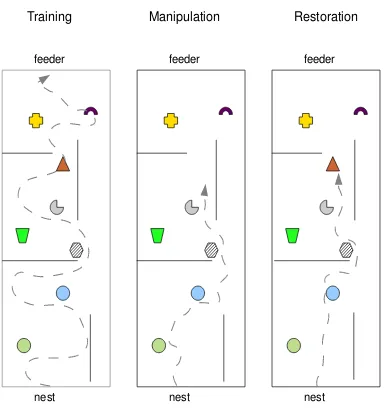
Both the real ant and the artificial forager calledSyntheticAntare made to forage for the feeder (food location) in an initially unknown environment starting from its nest. The environment contains many visual landmarks which could be used by the forager for navigation. After many foraging runs, some landmarks are displaced or removed. The forager is then made to forage in this manipulated environment. In the next foraging runs, the original landmark constellation is restored. This task allows to study and compare three key issues of autonomous navigation:

•learning landmark navigation in a dynamic environment

•behavior upon detection of landmark manipulation

•confidence adaptation depending on the reliability of the landmarks af-ter restoration.

See figure 2.9 for an illustration.

Real ant experiments in dynamic environments

A B

C

nest feeder

Training

nest feeder

Manipulation

nest feeder

Restoration

is important to note that in the real ant navigation experiments, the paper on the floor of the arena was replaced after each foraging run, in order to avoid the use of chemical cues by the ants.

Modeling and simulation environment

The modeling environment allows the input of the real ant trajectory for the simulated ant called the SyntheticAnt, allowing it to have the same perceptual input during foraging. Also free foraging behavior is available. The simulation replicates the real arena and the robot. It allows testing navigational paradigms before they are tested on the real robot. In this work we only consider the simulated robot.

We test the proposed navigational model on the simulated robot. As the neural implementation of the model is the very same for the simulated and the realSyntheticAnts, the transition from simulation to real world is readily manageable. More details of the experimental setup and the real robot version of theSyntheticAntare discussed in [74].

2.2.2

The extended model for mapless landmark

naviga-tion in dynamic environments

... DAC Contextual Layer LTM con te xt ual  seque nces Segment B C on te xt ua l L ay er pe rc ep tio n  m at ch in g LTM STM successful segment sequence segment =  landmark features +  HDA­set + segment weight current segment sequence memorized sequences co nte xtu al r ec all ­ h om ing ­ la nd m ark  na vig atio n A t3 t2 t1  sequence retention time w t3 t2 t1 S1 S2 G S1, S2: recalled landmark segments G: goal landmark segment recall of p1: path(S1,G)           and p2: path(S2,G)  probability distribution of  goal vector from memory  readout angle prob abi lit y relevance of p1 = f(t1, w1)) relevance of p2 = f(t2, w2) C G distance

Figure 2.10: (A) DAC Contextual Layer A segment contains the ex-tracted landmark features, an HDA-set and the segment weight. Segments are sequenced temporarily in the short-term memory (STM) whenever a landmark is encountered. Upon feeder detection, the contents of the STM are transferred into the long-term-memory (LTM). During recall phase (homing, landmark navigation), the LTM is matched against the current sensory events and an optimal trajectory is computed from recalled LTM segments. (B) Sequencing:During the foraging runs from the nest to the feeder, encountered landmarks are chained in the DAC contextual layer short-term memory (STM) together with the HDA set. Each LTM se-quence has a retention timetowing to thetransiencyof memory and each segment has a weightw. (C) Recall: During the recall phase, the HDA-sets starting from the recalled segment to the goal segment are combined to compute the optimal homing vector. When the recalled segment and the goal segment are on different LTM sequences, the segments from the recalled segment to the nest on one sequence, and the nest to the goal segment on the other are combined (such a combination is called path).

using it as a forward model, we only deal with the contextual layer.) These representations are used to plan ongoing behavior, and have been shown to be compatible with formal Bayesian models of decision making [112]. We use the DAC contextual layer to learn sequences of landmarks to-gether with their Heading Direction Accumulator (HDA) set. Using this the navigator can memorize several trajectories from the nest to feeder, leading through different landmarks. The DAC contextual layer recall mechanism is used when in the test scenario, a particular landmark is en-countered, to recall the vectors to other landmarks. The details of this mapless navigational strategy is discussed in the previous section [74]. In this section, we consider the use of DAC contextual layer and its recall mechanism as a forward model for learning to navigate in unknown and dynamic environments.

2.2.3

Dynamic memory consolidation using expectations

Cognitive psychology has recently begun to embrace a new position rec-ognizing memory as a highly dynamic process [79]. In this new view, remembering and forgetting are not merely transient processes; moreover they are achieved through a highly dynamic (re)consolidation process. Strong support for such a dynamic memory comes from animal neuro-science studies as reviewed in [79].

highly dynamic environments.

stable

memory memoryinstable consolidate

recall

acquire forget

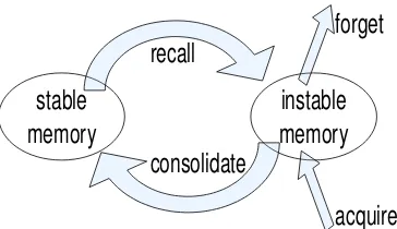
Figure 2.11: Dynamic Memory Reconsolidation Schema: As a mem-ory is acquired it enters the instable state and then is consolidated into the stable state. Nevertheless, memories in the stable state can reenter the instable state upon recall. Reconsolidation again stabilizes this memory that otherwise gets forgotten [79].

Transiency and confidence in memory sequences

We elaborate how transiency and confidence in memory traces are formu-lated for mapless navigation in uncertain environments. First we consider the situation, where the SyntheticAnt is kidnapped after many foraging runs and placed at an arbitrary visual landmark. The details of the mem-ory recall using the DAC contextual layer for mapless navigation can be consulted in section 2.1.7 [74]. Memory recall of the DAC contextual layer is used to compute an optimal path to another given landmark; we further refer to this as the memory answer. We define a vector V~ as a two dimensional vector indicating the angleγ and distanceψ of a given memory answer: V~ = [γ, ψ]T_{. Assuming that n LTM sequences were}

recalled, we are interested in computing the probability distribution:

where V~ is the vector indicating the goal,t is time, V~t

i is the vector

suggested by LTM sequence i, tret_i is retention time of LTM sequence

i and rseg_i is the segment relevance of the recalled segment of LTM se-quencei.

We look at the contribution of one LTM sequence i to the overall memory answer:

P(γψ|t, ~V_it, tret_i , r_iseg) (2.6) First, we consider equation 2.6 without the retention times:

P(γψ|t, ~V_it, r_iseg) (2.7)

Using conditional independence of angle and distance we get

P(γψ|t, ~V_it, r_iseg) = P(γ|t, ~V_it, r_iseg)

·P(ψ|t, ~V_it, r_iseg)

·P(t, ~V_it, r_iseg) (2.8)

whereV~_it= [γ_it, ψ_it]T. We formulateP(γ|t, ~V_it, rseg_i )andP(ψ|t, ~V_it, rseg_i )

as Gaussian distributions centered around the means γi and ψi

respec-tively with time dependent variances, signifying that higher weight seg-ments have a higher influence on the total memory answer as they have a smaller variance. This dynamically adapting variance is used to weight successful segments more and unsuccessful ones less.

P(γ|t, ~V_it, r_iseg) =N(γi,f1(rsegi )) (2.9) P(ψ|t, ~V_it, r_iseg) =N(ψi,f2(rsegi )) (2.10)

wheref1 andf2 are exponential growth functions of variance:

f1(x) =a1ek1(x) (2.11)

As all memory answers should be seen as equally probable and no correlations of distance, angle and retention-times of LTM sequences are known, we assume the uniform distribution:

P(t, ~V_it, rseg_i ) =U (2.13) Now we consider the contributions of all selected LTM sequences weighted by segment retention timestret

i :

P(V~|t, ~V₁t, tret₁ , r₁seg· · ·V~_nt, tret_n , rseg_n ) = X

i

tret

i ttot

P(γ|t, ~V_it, rseg_i )P(ψ|t, ~V_it, rseg_i )P(t, ~V_it, r_iseg) (2.14)

wherettot = Pitreti . Equation 2.14 signifies that the sequence

reten-tion times are used to weight the shares of LTM sequences to the final memory answer. In other words, sequences are weighted so that mem-ory acquired further back in the past is weighted less than more recent memory.

Building up confidencein uncertain environments

When a landmark (or feeder) at a known location ceases to be available or its position is manipulated, insects have been shown to exhibit search pat-terns that optimize rediscovery of the landmark (or feeder) [116]. We fur-ther refer to landmark manipulations of all kinds asmanipulation. It has also been proposed that such search patterns in insects could be modeled using L´evy walks [96]. L´evy walks are characterized by a distribution function

P(lj)∼l

−µ

j (2.15)

with 1 ≤ µ ≤ 3, where lj is the walk length. The direction of the

walk is drawn from a uniform distribution. The natural parameterµhas been shown to be optimal at the value2for modeling insectmanipulation

Here we propose a modified version of L´evy walk, to model the con-fidence building behaviorexhibited by ants upon manipulation. By con-fidence building behaviorwe mean the specific behavior exhibited by the animal once it detects the manipulation of a known landmark, namely the environment resampling strategy that seems to serve the purpose of re-building the confidenceabout the route to the feeder. The key idea is to propagate the initialization point of the L´evy walk towards the nest, so that the probability of encountering known landmarks is increased. Thus, the forager can slowly build upconfidenceabout the distance and direction to the navigational goal. The proposed version of L´evy walk is summarized in the pseudo-algorithm below:

while|con| ≤do

t ←0

whilet≤θdo

perf orm L´evy walk f rom i

upon landmark detection:update con

end while

ifi=nestthen

reset i to manipulation point else

propagate i towards nest end if

end while

where con is the mean confidence about the goal direction and dis-tance, i the current position at which the L´evy walk is initialized, andθ

ran-domly in the whole arena. This is strongly suggested by observed ant behavior in similar situations and is evaluated in our experiments.

Gm Gs Gr Δs Δm after traversal and  goal detection Gr: perceived goal Gs: goal expectation of segment Gm: memory answer la nd m ark  fe atu re s Recalled  Segment H D A   se t w se gm en t w eig ht expectation to perception  discrepancy ∆s used to  update segment weight w

angle dist

ance t3 t2 t1 t4 memory to perception  discrepancy ∆m is 

accounted for by retaining  the sequence with the 

newly traversed  landmarks in the LTM

Contextual Layer LTM

Figure 2.12: Expectation reinforcement for memory consolidation:

Discrepancy between expected paths and computed paths are used to con-solidate memory by means of setting LTM segment weights and writing new LTM sequences.

Adapting landmark reliability measure using expectations

To update the DAC LTM segment weight using the discrepancy, we use the exponential decay function

r_tseg₊₁ =rtsege−λd (2.16)

wheredis the discrepancy andtis time step. This causes the segment weight to fall exponentially from its current value if the discrepancy is high. Discrepancies are normalized (0 ≤ d ≤ 1) so that d = 1for the highest possible discrepancy (the length of the diagonal of the arena). The natural parameterλwas shown to optimally fit observed insect behavior at the value 2 [116]. The above decay is applied only if the discrepancy is above a fixed threshold. Otherwise, the segment weight is allowed to grow according to a linear function. In the following, we use the terms landmarkreliabilityandconfidenceinterchangeably.

2.2.4

Results

First we test the ability of the proposed model to learn the reliability of landmarks. For this purpose we test the simulated SyntheticAnt in an arena with 10 visual landmarks. During the foraging no landmark ma-nipulation were carried out. After that, during the test 9 of the 10 visual landmarks were displaced randomly in each run, i.e. there was only a single stable landmark. After the foraging runs, we test the feeder direc-tion and angle from the nest, computed as discussed earlier, using each of the 10 landmarks. Note that for this the distance and angle to the feeder from an arbitrary landmark is computed first using DAC contextual recall (as in [74]), which is then added to the vector leading from the nest to this landmark. This allows to visualize the belief of the forager in the reliability of each landmark as a probability distribution, as plotted in fig-ure 2.13. TheSyntheticAntlearns through expectation reinforcement that only landmark number 10 is stable. The evolution of the confidence in the landmarks are shown in figure 2.13 A (before the test runs), B (after 5 test runs) and C (after 10 test runs).

of landmark manipulations in the real ant experiment and in the simula-tion. We also use similar landmarks in the simulation as used in the ant experiments. Nevertheless, for simplicity we do not consider complex landmarks such as shadows, light direction etc. known to be used by real ants in the simulation. Our simulations run at about 30Hz on an Intel(R) Core(TM)2 Duo CPU 2.66GHz machine under openSUSE 10.3.

Table 2.2 shows the learned parameters of confidence in the individual landmarks, which corresponds to figure 2.13, C. The growing skewness of the distributions from left to right shows growing asymmetry in the distribution, indicating that the navigator increases confidence in some landmarks and decreases in some others.

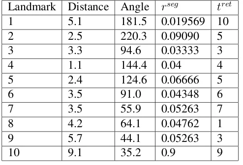
Table 2.2: Landmark stability learning experiment: the table shows the ten landmarks available in memory, the angle and distance from each landmark to feeder, the segment relevance of the segment containing the landmark (rseg_{) and the retention time (t}ret_{) of the memory sequence from}

which this landmark recalled.

Landmark Distance Angle rseg _tret

1 5.1 181.5 0.019569 10 2 2.5 220.3 0.09090 5 3 3.3 94.6 0.03333 3

4 1.1 144.4 0.04 4

5 2.4 124.6 0.06666 5 6 3.5 91.0 0.04348 6 7 3.5 55.9 0.05263 7 8 4.2 64.1 0.04762 1 9 5.7 44.1 0.05263 3

10 9.1 35.2 0.9 9

The segment retention time tret _{is the number of the latest foraging}

run in which the corresponding landmark was encountered, i.e. giving a high value to recent runs. The segment weight rseg _{is initialized to 1.}

distan ce (

)

manipulated landmarks

stable landmark

angle () 

distan ce (

)

angle ()  angle () 

distan ce (

)

p

ro

b

a

b

ili

ty

A B C

skewness = 0.0415 skewness = 1.1828 skewness = 2.4662

Figure 2.13: Expectation reinforcement for learning stable

land-marks: A)Before the test runs (but after several foraging runs)

the segment weight of landmark 1 is very low it has low influence on the overall answer. As shown in figure 2.13, the confidence for stable landmarks is reinforced and is higher than instable landmarks; i.e. the forager learns the stability of the landmarks. In short, higher frequency of landmark position manipulations lead to lower segment weights, meaning lower confidence represented by higher covariances of Gaussians. The stable landmark has a greater influence than instable ones on the overall memory readout (higher probability). The forager thus learns the stability of the individual landmarks. Therefore higher frequency manipulations of landmarks are reflected directly in the joint probability distribution with lower probabilities. In short, the higher the search intensity the lower the confidence.

Given the above result, we now investigate how theSyntheticAntcan regain its confidence, once its expectation is violated. Expectation is vio-lated when an expected landmark is missing or if a low confidence land-mark is encountered. As described before, theSyntheticAntfalls into the L´evy search mode and the intensity of the search is higher if the landmark is missing. We evaluate how confidence is regained with time and how the search intensity influences (figure 2.14). The θ value indicates the search intensity (θ3 > θ2 > θ1). The results show that the confidence is

regained with time, where high intensity searches allow to reach a higher confidence threshold in a shorter amount of time.

In figure 2.15B)the animal finds high discrepancy between its expec-tation and perception. This results in very low confidence and it performs correction maneuvers by going back towards the nest. The norms of the position density matrix, reflecting the task resolution times, for the real ant and the robot are shown in figure 2.16.

com-time [s]

co

nfide

nce a

s 

pr

oba

bi

lity