A fast algorithm for robust constrained clustering

A fast algorithm for robust constrained

clustering

Heinrich Fritza, Luis A. Garc´ıa-Escuderob, Agust´ın Mayo-Iscarb

a_{Department of Statistics and Probability Theory}

Vienna University of Technology

b_{Department of Statistics and Operations Research and IMUVA}

University of Valladolid

Abstract

The application of “concentration” steps is the main principle behind Forgy’s k-means algorithm and Rousseeuw and van Driessen’s fast-MCD algorithm. Despite this coincidence, it is not completely straightforward to combine both algorithms for developing a clustering method which is not severely affected by few outlying observations and being able to cope with non spherical ters. A sensible way of combining them relies on controlling the relative clus-ter scatclus-ters through constrained concentration steps. With this idea in mind, a new algorithm for the TCLUST robust clustering procedure is proposed which implements such constrained concentration steps in a computationally efficient fashion.

Keywords: Cluster Analysis, Robustness, Impartial trimming, Classification EM algorithm, TCLUST.

1. Introduction

Van Driessen, 1999). These two widely applied algorithms play a clear key role in Cluster Analysis and in Robust Statistics, respectively. The connec-tion between them mainly refers to the applicaconnec-tion of the so-called “concen-tration” steps. Roughly speaking, in these concentration steps, the closest observations to a given center are considered in order to update this center estimate, such that the algorithm searches for regions with a high concentra-tion of observaconcentra-tions.

A great drawback when using the k-means method is that it ideally searches for spherically scattered clusters with similar sizes. Further, the presence of a certain fraction of outlying observations could negatively affect its performance (see, e.g., Garc´ıa-Escudero et al., 2010).

Under the previous premises, it seems quite logical to try to combine the clustering ability ofk-means with the ability to robustly estimate covariance structures provided by the fast-MCD algorithm.

The trimmed k-means algorithm (Garc´ıa-Escudero et al., 2003) can be seen as a simple combination of k-means and fast-MCD algorithms, where spherical clusters are still assumed. In each concentration step, the propor-tion α of the most remote observations (considering Euclidean distances) to the previous k centers are discarded. Subsequently, k new centers are ob-tained by using the group means of the non-discarded observations. Note that the approach simplifies to the well-known Forgy’s k-means algorithm when the trimming level α is set to 0. More information on the trimmed k-means approach can be found in Cuesta-Albertos et al. (1997) and Garc´ıa-Escudero and Gordaliza (1999).

considering Mahalanobis distances (xi−mj)′Sj−1(xi−mj) (as the fast-MCD algorithm does) instead of Euclidean distances. In this case, the centers mj and the “scatter matrices” Sj (for j = 1, . . . , k) would be updated by com-puting sample means and sample covariance matrices of the non-discarded observations assigned to each group. Unfortunately, this “naive” combina-tion of algorithms does not provide sensible clustering results, since large clusters tend to “eat” smaller ones. This problem was already noticed in Maronna and Jacovkis (1974) in the untrimmed case (α= 0).

For avoiding this drawback, additional constraints are introduced, which limit the difference between the cluster scatters. In fact, many well-known clustering methods implement (implicitly and explicitly) such constraints. For example, the k-means method assumes the same spherical scatter for all the clusters.

Hathaway (1985), in a pioneering work on the mixture fitting frame-work, proposed constraining the relative differences between cluster scatters through a constantcthat controls the strength of the constraints. With this idea in mind, Garc´ıa-Escudero et al. (2008) introduces the TCLUST method which is based on controlling the relative sizes of the eigenvalues of the cluster scatter matrices.

to enforce the eigenvalue ratio constraints. This is clearly its computational bottle-neck because a complex optimization problem must be solved in each concentration step. To be more precise, a maximization of a (k×p)-variate function with (k×₂p) constraints needs to be solved (k stands for the num-ber of clusters and p for the data dimension). This makes the algorithm computationally unfeasible even for moderate values of k and/or p.

In this work, we present an algorithm for implementing the constrained concentration steps, which clearly speeds up the previous TCLUST algo-rithm and makes it computationally feasible for practical applications. This algorithm only requires the evaluation of a not very complex function 2pk+ 1 times in each concentration step.

The proposed algorithm can be seen as a Classification EM algorithm (Schroeder, 1976; Celeux and Govaert, 1992) and, more generally, as a gen-eralized k-means algorithm (Bock, 2007). Note that the proposed algorithm allows to exactly solve the (constrained) maximization step, which forces the trimmed likelihood target function to increase monotonically through the iterations.

An implementation of the algorithm described in this work is available through the R package tclust available at http://CRAN.R-project.org/ package=tclust. A description of how this R package can be used in prac-tical applications can be found in Fritz et al. (2012). In this work, we detail the algorithms internally applied by this package.

compared to other closely related ones in Section 5. Section 6 explains how this algorithm allows the practical application of exploratory tools which help us to decide on the number of clusters and the trimming level. Section 7 finally presents concluding thoughts.

2. Constrained robust clustering and TCLUST

Given a sample of observations {x1,· · · ,xn} in Rp and ϕ(·;µ,Σ), the probability density function of a p-variate normal distribution with meanµ

and covariance matrixΣ, we consider the following generalrobust constrained clustering problem for a fixed trimming level α:

Search for a partition R0, R1,· · · , Rk of the indices {1,· · · , n} with #R0 = ⌈nα⌉, centers m1,· · · ,mk in Rp, symmetric posi-tive semidefinite p×p scatter matrices S1,· · · ,Sk and weights p1,· · · , pk with pj ∈[0,1] and

∑k

j=1pj = 1, which maximizes k

∑

j=1

∑

i∈Rj

log(pjϕ(xi;mj,Sj)

)

. (2.1)

Depending on the constraints imposed on the weightspj and on the scat-ter matricesSj, the maximization of (2.1) forα = 0 leads to well established clustering procedures. For instance, assuming equal weights p1 = · · · = pk and scatter matrices S1 = · · · = Sk = σ2I with I being the identity matrix and σ > 0 yields the k-means method. The determinantal crite-rion introduced by Friedman and Rubin (1967) is obtained when assuming

p1 =· · ·=pkandS1 =· · ·=Sk=SwithSbeing a positive definite matrix.

The use of (2.1) assuming different weights pj goes back to Symons (1981) and Bryant (1991) and is known as the penalized Classification-Likelihood criterion.

Trimmed alternatives to the previously commented approaches can be constructed by introducing a trimming level α > 0 to (2.1), which yields “trimmed likelihoods”. This way, for instance, the trimmedk-means method in Cuesta-Albertos et al. (1997) extends k-means and the trimmed deter-minantal criterion in Gallegos and Ritter (2005) extends the deterdeter-minantal criterion. Note that⌈nα⌉observations (R0) are not taken into account when computing (2.1), and thus the harmful effect of outlying observations, up to a contamination level α, can be avoided. Gallegos and Ritter (2005) in-troduce the so-called “spurious outlier model” that theoretically justifies the use of trimmed likelihoods. It is also important to note that this robust clustering problem reduces to the fast-MCD method when assuming k = 1 (i.e. only partitioning the data into ⌈nα⌉ trimmed and ⌊n(1−α)⌋ regular observations).

In order to make the maximization of (2.1) a well defined problem, Garc´ıa-Escudero et al. (2008) proposed to additionally consider an eigenvalue ratio constraint on the scatter matrices S1,· · · ,Sk:

maxj,lλl(Sj) minj,lλl(Sj)

≤c, (2.2)

withλl(Sj) forl = 1,· · · , p, as the set of eigenvalues of the scatter matrixSj and c≥1 as a constant which controls the strength of the constraint (2.2).

The maximization of (2.1) under the eigenvalue ratio constraint (2.2) leads to the TCLUST problem introduced by Garc´ıa-Escudero et al. (2008). The smaller the value of c is, the stronger the restriction imposed on the solution, yielding the strongest constraint when c= 1.

Garc´ıa-Escudero et al. (2008) proves the existence of solutions for the pre-viously stated robust constrained clustering problem whenever some patho-logical (non-interesting for robust clustering) data configurations are ex-cluded. To be more precise, data configurations where all data points are concentrated in k points after deleting a fraction α of data points are ex-cluded.

The TCLUST method has good theoretical and robustness properties but no practically applicable algorithm is available yet when k×pis moderately large. To overcome this drawback, a computationally efficient algorithm for implementing this method will be described in the next section.

3. Algorithm

faster approach will be presented here. Further, an inaccuracy in the presen-tation of this algorithm will be corrected.

Starting with the three steps (E, C and M-) for the Classification EM algorithm described in Celeux and Govaert (1992), we propose the following algorithm:

E-step. For each observation xi and Dj(xi;θ) =pjϕ(xi;mj,Sj), the posterior probabilities

Dj(xi;θ)

∑k

j=1Dj(xi;θ)

for j = 1,· · · , k,

are computed, with θ = (p1,· · · , pk,m1,· · · ,mk,S1,· · · ,Sk) as the set of cluster parameters in the current iteration of the algorithm.

C-step. Each non-trimmed observation xi will be assigned to the cluster which provides maximum posterior probability. In order to implement the trimming procedure, the ⌈nα⌉observations xi with smallest values of

D(xi;θ) = max{D1(xi;θ),· · · , Dk(xi;θ)} (3.1)

are discarded as possible outliers (for this iteration).

M-step. The parameters are updated, based on the non-discarded observations and their cluster assignments. At this point, it is crucial to properly enforce the constraints on the cluster scatter matrices.

the largest (3.1) values are those with the smallest Mahalanobis distances (xi−mj)′Sj−1(xi−mj) (as considered in the concentration steps of the fast-MCD algorithm). When k >1, p1 =· · ·=pk and S1 =· · ·=Sk =σ2I, the observations with the largest (3.1) values are those with the smallest values of minj=1,···,k∥xi−mj∥2 (as considered in the (trimmed) k-means algorithm).

A more detailed presentation of the proposed algorithm is as follows:

1. Initialization: The procedure is initialized nstart times by selecting different θ0 _{= (p}0

1,· · · , p0k,m10,· · · ,m0k,S 0

1,· · · ,S 0

k). For this purpose, we propose to randomly selectk×(p+1) observations and to accordingly computekcluster centersm0

j andkscatter matricesS 0

j from the chosen data points. If needed, the cluster scatter matrix constraints are applied to these S0_j (as will be described in Step 2.2). Weights p0

1,· · · , p0k in the interval (0,1) and summing up to 1 are also randomly chosen. 2. Concentration step: The following steps are executed until

conver-gence (i.e., θl+1 =θl) or a maximum number of iterations iter.maxis reached.

2.1. Trimming and cluster assignments (E and C-steps): Based on the current parametersθl_{= (p}l

1,· · · , plk,m1l,· · · ,mlk,S l

1,· · · ,S l k) the ⌈nα⌉ observations with the smallest values of D(xi, θl) are discarded. Each remaining observation xi is then assigned to a cluster j such that Dj(xi, θl) =D(xi, θl). This yields a partition

R0, R1,· · · , Rk of {1,· · · , n} holding the indexes of the trimmed

2.2. Update parameters (M-step): Given nj = #Rj, the weights are updated by

pl+1_j =nj/[n(1−α)] and the centers by the sample means

ml+1_j = 1

nj

∑

i∈Rj

xi.

Updating the scatter estimates is more difficult, as the sample covariance matrices

Tj =

1 nj

∑

i∈Rj

(xi−ml+1j )(xi−ml+1j )′,

may not satisfy the specified eigenvalue ratio constraint. In this case, the spectral decomposition of Tj = U′jDjUj is consid-ered, withUj being an orthogonal matrix andDj = diag(dj1, dj2,

· · · , djp) a diagonal matrix. Let us consider truncated eigenvalues

defined as

dm_jl =

        

djl if djl∈[m, cm] m if djl< m cm if djl> cm

, (3.2)

withmas some threshold value. The scatter matrices are updated as

Sl+1_j =U′_jD∗_jUj,

with D∗_j = diag(dmopt

j1 , d mopt

j2 ,· · · , d mopt

jp

)

and mopt minimizing

m7→ k ∑ j=1 nj p ∑ l=1 (

log(dm_jl)+ djl dm jl

)

As it will be shown in Proposition 3.2, this expression has to be evaluated only 2kp+ 1 times to exactly find the minimum. 3. Evaluate target function: After the concentration steps, the value of the

target function (2.1) is computed. The parameters yielding the highest value of this target function are returned as the algorithm’s output.

The proposed algorithm can be used to solve the maximization of (2.1) when assuming equal weights p1 = · · · = pk, by simply setting all weights constantly to pl

j = 1/k within each iteration. Little changes to this algo-rithm would also yield a generalized version of a robust clustering method introduced by Gallegos (2002) but relaxing the constraint det(S1) = · · · = det(Sk) thereby considering determinant ratio constraints as in Section 3.9.1 of McLachlan and Peel (2000). In a similar way, the presented algorithm can also be adapted to develop EM algorithms for constrained mixture fitting problems.

per-formance of the proposed algorithm will be given in Section 4.

The main novelty of this algorithm, compared to Garc´ıa-Escudero et al. (2008), is how constraints on the eigenvalue ratio are enforced. Equation (3.4) in Garc´ıa-Escudero et al. (2008) constrains eigenvalues by solving the minimization problem

(d∗₁₁, d∗₁₂,· · · , d∗_jl,· · · , d∗_kp)7→ k

∑

j=1 nj

p

∑

l=1

(

log(d∗_jl)+ djl d∗_jl

)

, (3.4)

under the restriction

(d∗₁₁, d∗₁₂,· · ·, d_jl∗,· · · , d∗_kp)∈Λ, (3.5)

with Λ as the cone

Λ ={d∗_jl :d∗_jl≤c·d∗_rs for every j, r∈ {1,· · · , k} and l, s∈ {1,· · · , p}}. (3.6) This is clearly a more complex problem than minimizing (3.3), as its complex-ity tremendously increases with the number of clusters k and the dimension p. The problem of minimizing (3.4) in Λ was translated into a quadratic pro-gramming problem, which was approximately solved by recursive projections onto cones (Dykstra, 1983). These recursive projections must be carried out in each concentration step and, thus, the algorithm becomes extremely slow and even unfeasible for moderately high values of k and/or p. Moreover, there was a mistake in Garc´ıa-Escudero et al. (2008), as the termnj in (3.4) was omitted and, thus, the algorithm proposed there can only be applied to similarly sized clusters.

Proposition 3.1. If the sets Rj, j = 1,· · · , k, are kept fixed, the maximum of (2.1) under constraint (2.2) can be obtained through the following steps:

(i) The best choice of pj is pj =nj/⌊n(1−α)⌋ with nj = #Rj. (ii) Fixed pj as given in (i), the best choice for mj is mj =

∑

i∈Rjxi/nj.

(iii) Fixed the eigenvalues for the matrix Sj and the optimum values given

in (i) and (ii) for pj and mj, the best choice for the set of unitary eigenvectors is the set of unitary eigenvectors of the sample covariance

matrix of the observations in Rj.

(iv) With the optimal selections from (i), (ii) and (iii), ifdjl are the eigen-values of the sample covariance matrix, the best choice for the truncated

eigenvalues dmopt

jl is as in (3.2) with mopt minimizing function (3.3). Then, the best choice for the scatter matrix Sj is obtained with the

eigenvectors of the sample covariance matrix of the observations in Rj and with the optimally truncated eigenvalues.

Proof. The proofs of statements (i), (ii) and (iii) are included in the proof

of Proposition 4 in Garc´ıa-Escudero et al. (2008).

Let us consider the spectral decomposition of the sample covariance ma-trices of observations given by:

Tj =

1 nj

∑

i∈Rj

(xi−mj)(xi−mj)′ =U′jDjUj, (3.7)

where Uj are orthogonal matrices and Dj = diag(dj1, dj2,· · · , djp) are diag-onal matrices.

and pj are those given by (i) and (ii). Analogously to the previous decom-position of the sample covariance matrices, matrices Sj can be split up into

Sj =V′jD∗jVj withVj orthogonal matrices andD∗j = diag(d∗j1, d∗j2,· · · , d∗jp) diagonal matrices. Statement (iii) tells us that eigenvectors of the optimal constrained matrices Sj must be exactly the same as the eigenvectors of the unrestricted sample covariance matrices in (3.7) (i.e., we can set Uj =Vj). We just need to search for the optimal eigenvalues {d∗_j,l} to obtain the opti-mally constrained scatter matrices Sj =U′jD∗jUj.

Given the eigenvalues{dj,l}, the optimal{d∗j,l}are obtained by minimizing expression (3.4) when {d∗_j,l} ∈ Λ with Λ as defined in (3.6). The proof of this claim follows from the proof of Proposition 4 in Garc´ıa-Escudero et al. (2008), with the only difference that expression (3.4) now contains the cluster sizes nj, whereas Equation (3.4) in the mentioned article wrongly did not.

Note that Λ can be written as

Λ = ∪ m≥0

Λm with Λm = ∪ m≥0

{

d∗_jl:m≤d∗_jl ≤cm}.

Thus, for globally minimizing expression (3.4) in Λ, we need to be able to minimize it when{d∗_j,l} ∈Λm for every possible valuem >0. The minimiza-tion (for a fixed value of m) can be significantly simplified by considering truncated eigenvalues d∗_jl =dm

jl like those in (3.2).

Possible singularities inTj are not a problem, provided that not all values of djl are 0 at the same time. Under this mild assumption, it is easy to see thatm >0 and this prevents that any value ofd∗_jl drops to 0 (i.e. no singular clusters are obtained after the truncation of the eigenvalues).

eigenvalues) just by evaluating the function (3.3) 2pk+ 1 times:

Proposition 3.2. Let us consider e1 ≤e2 ≤ · · · ≤e2kp obtained by ordering the following 2pk values:

d11, d12,· · · , djl,· · · , dkp, d11/c, d12/c,· · · , djl/c,· · · , dkp/c,

and, f1,· · · , f2kp+1 any values satisfying:

f1 < e1 ≤f2 ≤e2 ≤ · · · ≤f2kp ≤e2kp < f2kp+1.

We can choose mopt as the value of:

mi =

∑k j=1nj

( ∑p

l=1djl(djl< fi) + 1_c

∑p

l=1djl(djl> cfi)

) ∑k

j=1nj

( ∑p

l=1((djl < fi) + (djl> cfi))

) ,

i= 1,· · ·,2kp+ 1, yielding the minimum value of (3.3).

Proof. Firstly, let us rewrite the target function (3.3) as

f :m 7→ k

∑

j=1 nj

[_∑p

l=1

(log(m) +djl/m)(djl< m) (3.8)

+ p

∑

l=1

(log(djl) + 1)(m≤djl < cm)

+ p

∑

l=1

(log(cm) +djl/cm)(djl > cm)

]

.

Sincef is a continuously differentiable function, it minimizes in one of its critical values, which satisfies the following fixed point equation:

m∗ =

∑k

j=1(sj(m∗) +tj(m∗)/c)

∑k

with

rj(m) = p

∑

l=1

((djl< m) + (djl> cm)),

sj(m) = p

∑

l=1

djl(djl < m) andtj(m) = p

∑

l=1

djl(djl > cm).

Functions rj,sj and tj take constant values in the intervals (−∞, e1],(e1, e2],

· · · ,(e2k,∞). Therefore, we only need to evaluate (3.8) at the 2kp+ 1 values

m1,· · · , m2kp+1.

4. Simulation study

In this section, a small simulation study is presented, investigating the effect of the choice of parameters iter.max(number of concentration steps) and nstart (number of random initializations) on the performance of the algorithm.

A so-called M5 type data set is considered, which is based on the “M5 scheme” as introduced in Garc´ıa-Escudero et al. (2008). These simulatedp≥ 2 dimensional data sets consist of three partly overlapping clusters generated from three p-variate normal distributions with means

µ₁ = (0, β,0, . . . ,0),µ₂ = (β,0, . . . ,0) and µ₃ = (−β,−β,0, . . . ,0),

with β ∈R+ _{and covariance matrices}

−20 −10 0 10 20 −20 −10 0 10 (a) M5Data Outlier type: 1 (uniformly distributed)

−20 −10 0 10 20

−20

0

20

40

(b) M5Data Outlier type: 2 (linear)

(c) Classification k=3, α =0.1

−20 −10 0 10 20

−20

−10

0

10

(d) Classification k=3, α =0.1

−20 −10 0 10 20

−20

0

20

40

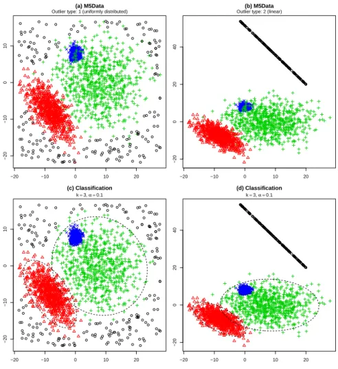
Figure 1: An M5 type data set in two dimensions with uniformly distributed outliers (a)

and outliers restricted to a line (b). Plots (c) and (d) show the corresponding clustering

results obtained bytclust.

Σ3 =

          

15 −10 0 . . . 0

−10 15 0 . . . 0 0 0 1 . . . 0

..

. ... ... . .. 0

0 0 0 0 1

The parameter β specifies how strong the clusters overlap, i.e. smaller values (e.g. 6) yield heavily overlapping clusters, whereas larger values (e.g. 10) yield a better separation of the clusters and thus a problem which is easier to solve. Theoretical cluster weights are fixed as (0.2,0.4,0.4), implying that the first cluster size is half the size of clusters two and three. Two further different types of outliers are considered which are added to the data:

Type 1: Uniformly distributed outliers in the bounding box of the data. Type 2: Uniformly distributed outliers restricted to a random hyperplane of dimension p−1.

All outliers are drawn under the restriction that the squared Mahalanobis distance of each outlier with respect to all three clusters must be larger than the 0.975 quantile of the chi-squared distribution with p degrees of freedom. Choosing a number of observations n = 2000, parameters p = 2 and β = 8 and a 10% outlier portion results in data sets as shown in Figure 1 (a) and (b) with outlier types 1 and 2 respectively. Considering outlier type 2 in a two dimensional data set reduces the space of the outliers to a line as seen in the mentioned figure. Panels (c) and (d) in the same figure show the corresponding cluster results computed with an R implementation of the described algorithm from package tclust. Apparently, the cluster structure is captured nicely by the algorithm; however, at the boundaries and overlapping regions of the clusters, some differences between the theoretical and the computed cluster assignment can be noticed.

2 4 6 8 12 16 24 32 64 X 20 40 60 80 (a) Error iter.max

Classification Error [%]

Outlier type: 1 (uniformly distributed)

2 4 6 8 12 16 24 32 64 X

20 40 60 80 (b) Error iter.max

Classification Error [%]

Outlier type: 2 (linear)

2 4 6 8 12 16 24 32 64 X

0.2 0.5 1.0 2.0 5.0 10.0 20.0 (c) Runtime iter.max Runtime [Seconds]

Outlier type: 1 (uniformly distributed)

2 4 6 8 12 16 24 32 64 X

0.2 0.5 1.0 2.0 5.0 10.0 20.0 (d) Runtime iter.max Runtime [Seconds]

Outlier type: 2 (linear)

Figure 2: Classification errors and runtimes of thetclustalgorithm applied to simulated

M5 type data sets for different values of iter.max and nstart = 32 when p= 10 and

β = 6 are fixed.

for each of these settings, a very precise “reference result” has been com-puted with parameters iter.max = 10000 and nstart = 200. All simula-tions were run on an AMD Phenom II X6 1055T at 2.8GHz.

Figure 2 shows the box plots of the classification errors in percent and runtimes for different values of iter.max and the two outlier types, using nstart = 32, p = 10 and µ = 6. The label “X” at the very right of each plot represents the “reference result”, which is assumed to be very close to the theoretically optimal solution. Differences between the outlier types can be seen, as in panel (a) a value of iter.max = 24 already gives a result very similar to the reference. On the other hand, in panel (b), with the outliers restricted to a hyperplane of dimension p−1, even a value iter.max = 64 yields three out of 100 solutions which apparently differ from the results in the reference solution “X”.

2 4 6 8 12 16 24 32 64 X 10 20 30 40 50 60 Error nstart

Classification Error [%]

Outlier type: 1 (uniformly distributed)

2 4 6 8 12 16 24 32 64 X

10 20 30 40 50 60 Error nstart

Classification Error [%]

Outlier type: 2 (linear)

2 4 6 8 12 16 24 32 64 X

0.05 0.10 0.20 0.50 1.00 2.00 5.00 20.00 Runtime nstart Runtime [Seconds]

Outlier type: 1 (uniformly distributed)

2 4 6 8 12 16 24 32 64 X

0.05 0.10 0.20 0.50 1.00 2.00 5.00 20.00 Runtime nstart Runtime [Seconds]

Outlier type: 2 (linear)

Figure 3: Classification errors and runtimes of thetclustalgorithm applied to simulated

M5 type data sets for different values of nstart and iter.max= 24 when p= 10 and

β = 6 are fixed.

is not the case with the first outlier scheme. Although the cluster structure can be found quickly, and most of the observations are assigned correctly, the outliers located in the outer regions of the clusters make it more difficult for the algorithm to converge.

and the parameters iter.max = 24, p= 10 and µ= 6 are fixed. When ap-plying the algorithm on data contaminated with the first outlier type, results computed with nstart = 24 are almost equal to the reference solution “X” as shown in panel (a). However, when the second outlier type is considered, even nstart = 64 is not sufficient to obtain a completely converged solu-tion. The corresponding runtimes, as shown in Figure 3 (c) and (d), depend linearly on the parameter nstart, as expected. Due to the earlier conver-gence of the algorithm, when contamination of the second type is present (as commented before), runtimes in panel (d) are slightly lower than in panel (a).

Figure 4 gives classification errors (a) and runtimes (b) for different values of β andp, the first outlier type and valuesiter.max= 64 andnstart = 64 fixed. As with increasing β the clusters are more easily separable, a larger value of β yields smaller classification errors. Due to the better separation of the clusters, the algorithm converges faster when β is large, resulting in lower runtimes.

Also, larger values of p decrease the classification error, as in higher di-mensional space the clusters are separated more clearly. In addition, an increase in the number of dimensions clearly increases the runtimes, which is expected due to the algorithm structure.

5. Relationships with other approaches

2 6 10 2 6 10 2 6 10 0 2 4 6 8 10 12

Classification Error Comparison

p

µ 6 8 10

_________ _________ _________ Equal Weights

2 6 10 2 6 10 2 6 10

0 2 4 6 8 10 12

Classification Error Comparison

p

µ 6 8 10

_________ _________ _________ Non−equal Weights

6 8 10 6 8 10 6 8 10

1 2 3 4 5 6 7 Runtime Comparison p µ

2 6 10

_________ _________ _________ Equal Weights

6 8 10 6 8 10 6 8 10

1 2 3 4 5 6 7 Runtime Comparison p µ

2 6 10

_________ _________ _________ Non−equal Weights

Figure 4: Classification errors and runtimes of thetclustalgorithm applied to simulated

M5 type data sets for different values of p and β and when values nstart = 64 and

iter.max= 64 are fixed.

procedure for solving them have key importance in the presented approach to robust clustering. Note that this yields a wide range of different cluster-ing solutions dependcluster-ing on the choice of constant c. These solutions range from almost spherical clusters when cis close to 1 to more unrestricted ones when cis huge. The researcher may choose from among them, depending on the clustering application in mind. Moreover, since both approaches share a similar type of target function (i.e., (2.1) with p1 = · · · = pk), it is easy to see that Neykov et al. (2007)’s target function is unbounded too and, if no constraints are posed, certain precautions in the associated algorithm are clearly needed in order to avoid the degeneration of the clustering solution. Neykov et al. (2007) also considers other interesting finite mixtures statistical problems where trimmed likelihoods can be successfully applied if robustness is a major concern.

Gallegos and Ritter (2009) have also considered a trimmed likelihood ap-proach with scatter matrix constraints. They propose to apply Hathaway (1985)’s original extension of his univariate constraints to multivariate prob-lems by constraining

min

l 1≤minh̸=j≤kλl(ShS

−1 j )≥

1

c with c≥1. (5.1)

the smaller cluster sizes, which implies solving a λ-assignment problem in the concentration steps.

In a mixture fitting framework without trimming, Ingrassia and Rocci (2007) proposed algorithms for addressing constrained mixture likelihood maximization. They give an interesting discussion starting from the con-straint (5.1) and ending with the same type of concon-straints as in (2.2). They propose an algorithm based on truncating scatter matrices eigenvalues when lower and upper bounds on these eigenvalues are known. Relaxing this as-sumption, when no suitable external information is available for bounding them, they also consider a bound on the ratio of the eigenvalues. However, their algorithm for this last proposal does not directly maximize the likeli-hood as is done in Step 2.2 of our algorithm. Rather, it is based on obtaining iterative estimates of a lower bound on the scatter matrices eigenvalues η needed in order to properly truncate the eigenvalues.

for noise, which explains its good robustness performance (Ruwet et al., 2012a,b).

6. Computation of Classification Trimmed Likelihood curves

One of the main motivations for a fast algorithm lies in the graphical tools introduced in Garc´ıa-Escudero et al. (2011) (see also Fritz et al., 2012), which help to make appropriate choices for the number of clusters k and the trimming levelα. The practical application of these tools, as e.g. the Classifi-cation Trimmed Likelihood curves, implies solving many TCLUST problems for different values ofαandk. This clearly turns out to be unfeasible without a computationally efficient algorithm at hand.

Of course, the determination of k and α is not a well-defined problem and, usually, several choices are arguable for these two parameters. For instance, the question of whether small subsets of isolated observations are actually clusters or only outliers is in many cases philosophical and usually related to the context in which a clustering problem is considered. In any case, the Classification Trimmed Likelihood curves provide helpful guidance for obtaining a small set of sensible choices for k and α which have to be carefully evaluated by the researcher.

0.00 0.05 0.10 0.15 0.20

−15000

−13000

−11000

(a) CTL curves

α

Objectiv

e Function V

alue

Restriction Factor = 50

55 55 55 55 55 55 55 55 55 55 5 4 44 44 44 44 44 44 44 44 44 44 3 33 33 33 3 3 3 33 33 33 33 33 3 22 22 22 2 2 2 2 2 22 22 22 22 22 1 1 1 1 1 1 1 1 1 1 11 11 11 11 11 1

(b) k=4 and alpha = 0

−20 −10 0 10 20

−20

0

20

40

Figure 5: (a) Classification Trimmed Likelihood curves for a data set like in 1,(b) and (d).

(b) Clustering solution for this data set whenk= 4 andα= 0.

α = 0.1 is considered. A detailed discussion on the interpretation of the Classification Trimmed Likelihood is given in Garc´ıa-Escudero et al. (2011) and Fritz et al. (2012).

7. Conclusions

A computationally feasible algorithm for robust heterogeneous clustering has been presented. The keystone of the proposed algorithm is the con-sideration of constrained concentration steps which combine elements of the fast-MCD algorithm with Forgy’sk-means algorithm, but enforce constraints on the ratio of the scatter matrices’ eigenvalues. This is done by additionally evaluating an explicit function at 2kp+ 1 values within each concentration step. The presented algorithm was implemented in the R package tclust.

References

Bock, H.-H., 2007. Clustering methods: A history of k-means algorithms. In: Brito, P., Bertrand, B., Cucumel, G., de Carvalho, F. (Eds.), Selected Contributions in Data Analysis and Classification. Studies in Classifica-tion, Data Analysis, and Knowledge OrganizaClassifica-tion, Berlin, Heidelberg, pp. 161–172.

Bryant, P., 1991. Large-sample results for optimization-based clustering methods. J Classif 8, 31–44.

Cuesta-Albertos, J., Gordaliza, A., Matr´an, C., 1997. Trimmed k-means: an attempt to robustify quantizers. Ann Stat 25, 553–576.

Dykstra, R., 1983. An algorithm for restricted least squares regression. J Am Stat Assoc 78, 837–842.

Forgy, E., 1965. Cluster analysis of multivariate data: efficiency versus inter-pretability of classifications. Biometrics 21, 768–780.

Fraley, C., Raftery, A. E., 1998. How many clusters? which clustering method? answers via model-based cluster analysis. The Computer J 41 (8), 578–588.

Friedman, H., Rubin, J., 1967. On some invariant criterion for grouping data. J Am Stat Assoc 63, 1159–1178.

Fritz, H., Garc´ıa-Escudero, L., Mayo-Iscar, A., 2012. tclust: An r package for a trimming approach to cluster analysis. J Stat Softw 47 (12).

URL http://www.jstatsoft.org/v47/i12

Gallegos, M., Ritter, G., 2005. A robust method for cluster analysis. Ann Stat 33, 347–380.

Gallegos, M., Ritter, G., 2009. Trimming algorithms for clustering contami-nated grouped data and their robustness. Adv Data Anal Classif 10, 135– 167.

Gallegos, M. T., 2002. Maximum likelihood clustering with outliers. In: Ja-juga, K., Sokolowski, A., Bock, H. (Eds.), Classification, Clustering and Data Analysis: Recent advances and applications. Springer-Verlag, pp. 247–255.

Garc´ıa-Escudero, L., Gordaliza, A., 1999. Robustness properties of k-means and trimmedk-means. J Am Stat Assoc 94, 956–969.

Garc´ıa-Escudero, L., Gordaliza, A., Matr´an, C., 2003. Trimming tools in exploratory data analysis. J Comput Graph Stat 12, 434–449.

Garc´ıa-Escudero, L., Gordaliza, A., Matr´an, C., Mayo-Iscar, A., 2008. A general trimming approach to robust cluster analysis. Ann Stat 36, 1324– 1345.

Garc´ıa-Escudero, L., Gordaliza, A., Matr´an, C., Mayo-Iscar, A., 2010. A review of robust clustering methods. Adv Data Anal Classif 4, 89–109.

Garc´ıa-Escudero, L., Gordaliza, A., Matr´an, C., Mayo-Iscar, A., 2011. Ex-ploring the number of groups in robust model-based clustering. Stat Com-put 21, 585–599.

Hathaway, R., 1985. A constrained formulation of maximum likelihood esti-mation for normal mixture distributions. Ann Stat 13, 795–800.

Hennig, C., 2004. Breakdown points for maximum likelihood-estimators of location-scale mixtures. Ann Stat 32 (4), 1313–1340.

Maronna, R., Jacovkis, P., 1974. Multivariate clustering procedures with variable metrics. Biometrics 30, 499–505.

McLachlan, G., Peel, D., 2000. Finite mixture models. Wiley Series in Prob-ability and Statistics, New York.

Neykov, N., Filzmoser, P., Dimova, R., Neytchev, P., 2007. Robust fitting of mixtures using the trimmed likelihood estimator. Comput Stat Data An 52, 299–308.

Rousseeuw, P., Van Driessen, K., 1999. A fast algorithm for the minimum covariance determinant estimator. Technometrics 41, 212–223.

Ruwet, C., Garc´ıa-Escudero, L. A., Gordaliza, A., Mayo-Iscar, A., 2012a. The influence function of the tclust robust clustering procedure. Adv. Data Anal. Classif 6 (2), 107–130.

Ruwet, C., Garc´ıa-Escudero, L. A., Gordaliza, A., Mayo-Iscar, A., 2012b. On the breakdown behavior of robust con-strained clustering procedures. Submitted, preprint avilable at http://orbi.ulg.ac.be/handle/2268/104215.

URL http://orbi.ulg.ac.be/handle/2268/104215

Schroeder, A., 1976. Analyse d’un m´elange de distributions de probabilits de mˆeme type. Rev Statist Appl 24, 39–62.