From raster to vector cellular automata models: a new approach to simulate urban growth with the help of graph theory

Texto completo

(1)BIBLIOTECA. Document downloaded from the institutional repository of the University of Alcala: http://dspace.uah.es/dspace/. This is a postprint version of the following published document: BARREIRA-GONZÁLEZ, P., GÓMEZ-DELGADO, M. and AGUILERABENAVENTE, F., 2015. From raster to vector cellular automata models: a new approach to simulate urban growth with the help of graph theory. Computers, Environment and Urban Systems, vol. 54, pp. 119-131 Available at http://dx.doi.org/10.1016/j.compenvurbsys.2015.07.004 © 2015 Elsevier. (Article begins on next page). This work is licensed under a Creative Commons Attribution-NonCommercial-NoDerivatives 4.0 International License..

(2) Title: From raster to vector cellular automata models: a new approach to simulate urban growth with the help of graph theory. Keywords: cellular automata, urban growth, graph theory, vector, simulation models. 1. Introduction Land use change, and urban growth dynamics in particular, are two of the phenomena that have contributed to land transformation in recent times (Seto et al., 2011). These kinds of change have a major environmental impact wherever they occur, with loss of natural land and the alteration of natural systems being two of the most significant consequences (Alberti & Marzluff, 2004; Berling-Wolff & Wu, 2004; Lauf et al., 2012). Studies of land use change as a dynamic system have enabled researchers to define the components and interrelations (Macgill, 1986) from which land use change emerges (Itami, 1994). One good way to describe these systems is to model their behaviour using tools that enable a spatial simulation of their associated dynamics (Aljoufie et al., 2013; Jantz et al., 2010; White, 1998). Urban growth represents one of the most significant land use changes, and simulation models constitute an essential tool for understanding the behaviour of expanding urban systems and determining their main characteristics, such as emergence, self-similarity, self-organisation and non-linear behaviour (Barredo et al., 2003; Frankhauser, 1998; Portugali, 2000). These models can be used to reproduce the dynamics related to these kind of systems (e.g. Benenson & Torrens, 2004), explore the factors that act as driving forces (e.g. Jokar Arsanjani et al., 2013; Leao et al., 2004), analyse urban growth patterns (e.g. Aguilera et al., 2011; Shafizadeh Moghadam & Helbich, 2013) and how they affect land (e.g. Mitsova et al., 2011), and lastly, study future consequences derived from several scenarios (e.g. Santé et al., 2010; Verburg et al., 2004; Zhang et al., 2011). A wide diversity of tools, approaches and spatial resolutions can be used to simulate urban dynamics: depending on the simulation method employed, these include Cellular Automata (CA) based models, Artificial Neural Networks, Fractal Modelling, Linear/Logistic Regression, Multicriteria Evaluation Techniques, Agent Based models and Decision Tree Modelling. Of these, the most widely used models over the last two decades have been CA-based models (see Triantakonstantis & Mountrakis, 2012; Santé et al., 2010). The main reasons for their success are their simplicity, flexibility, transparency and intuitiveness. They are also able to accurately reproduce emerging complex dynamics such as cities (Liu, 2012; White & Engelen, 1993). Nevertheless, several aspects of urban growth modelling have not yet been satisfactorily solved through the use of CA-based models, such as the representation of time built into model ticks, the introduction of randomness, raster cellular space (which does not take into account the real structure of the land) or the use of scales that are inappropriate for urban or regional planning. As a consequence, only a few models have been integrated into decision-making processes in planning (Triantakonstantis & Mountrakis, 2012). The CA-based models that have proliferated most to date are those which represent space using a raster surfaces (Barredo et al., 2004; Batty, 1998; Dietzel & Clarke, 2004; Li et al., 2008; Sante et al., 2010; White & Engelen, 1993; Wu, 2002). This method of representation is.

(3) strongly influenced by remote sensing (O'Sullivan & Torrens, 2000), in which satellite or aerial images represent the geographical space as a set of pixels (cells). This has been the most widely used format in this kind of model, partly due to its powerful spatial analysis capabilities and its capacity for mathematical calculation, yielding an appreciable reduction in computational time. However, an important question arises during the modelling process: is it appropriate to use raster surfaces in urban growth simulations? Urban space transformations do not follow the pattern of a regular structure such as that used in a raster data model; instead, they usually fit into the pre-existing land structure (basically plots or land parcels) so that it is irregular parcels which change rather than regular cells. Therefore, the use of regular cells as the minimum space representation units may be excessively simple in some cases and model outputs can be sensitive to cell size (Jantz & Goetz, 2005; Ménard & Marceau, 2005; Moreno et al., 2009; Pinto & Antunes, 2010). Consequently, although a raster surface may be appropriate for urban growth simulation on large study areas; this representation is to some extent less attractive when the aim is to describe an urban system and its associated dynamics at a more reduced extent, close to urban planning scales (Bardají, 2011). At this level, the use of the real (and irregular) spatial units employed in urban planning could help to build a more realistic model. In the Spanish planning practice the urban planning units are the existing cadastral parcel. Therefore, their use is not only a scale issue; they constitute a more realistic representation of the spatial reference unit. To address these two difficulties, the present article describes the implementation of a CA-based urban growth model prototype to explore the viability of vector land representation at a municipal scale. Irregular space structure was based on cadastral parcels (also known as plots), which constitute the geographical space division (according to land property) used in urban planning. Thus, the use of this structure to simulate urban growth will yield models capable of working at a scale closer to that employed in urban planning. Attaining this goal necessarily involves a significant relaxation of the formal structure of CAbased models. Irregular space representation entails implementing CA-based models in vector format; thus, it was necessary to adopt a computational solution since the use of this kind of format involves high computational costs. This was addressed through the use of graph theory, by abstracting vector representations to graphs. The prototype was entirely developed in Python (Van Rossum & Drake Jr, 2008), currently the most widely used open-source programming language for GIS. It has been tested in Los Santos de la Humosa, a municipality within the Community of Madrid, one of the most urbanised areas in Spain in recent decades. We do not expect to reproduce past tendencies or dynamics in that region in this stage of the modelling process. The purpose of the test is to verify the computational and operational viability of the prototype. The present article is organised as follows: the conceptual basis of CA-based modelling and its relaxation is described in section 2. In section 3, the prototype is presented; subsection 3.1 describes the area where the prototype was tested and the input data, 3.2 defines the conceptual basis of the prototype, 3.3 details how the vector structure is abstracted to a graph and 3.4 outlines implementation of the prototype. Section 4 presents the results and the discussion and finally, the conclusions are given in section 5. 2. CA-based model structure and its relaxation as the basis of a new prototype..

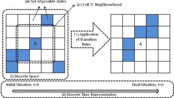
(4) 2.1. Conceptual basis of CA. Over the last few decades, several definitions of 'Cellular Automata' have appeared in the literature (Benenson & Torrens, 2004; Ménard & Marceau, 2005; Torrens & O'Sullivan, 2001; White, 1998; White & Engelen, 2000; Wolfram, 1984; Wu et al., 2009). In general, CA can be considered as a mechanism that reproduces processes whose characteristics change over time based on their status, rules and inputs (Benenson & Torrens, 2004). Wolfram (1984) proposed a more detailed description of the 5 main characteristics of CA: (i) discrete space representation, (ii) discrete time representation, (iii) each cell has one state from a set of possible states, (iv) transition rules depend only on the neighbourhood of a cell and its state, and finally, (v), the state of the cells changes according to the same transition rules (Figure 1).. Figure 1: Main CA characteristics proposed by Wolfram (1984). The figure shows a CA in its initial state (t=0) and its evolution until the final situation (t=n).. CA trace their origins to the 1940s when Stanislaw Ulam and Konrad Zuse established the theoretical basis of what they called 'computing spaces' for representing discrete physical systems, partially based on the work developed by Alan Turing (1936). Subsequently, John Von Neumann gave shape to these theories (Itami, 1994) by defining the CA (originally 'cellular space') as we currently know them, implementing the neighbourhood factor. As a result of these seminal works, the development and use of CA continued, with the Game of Life by John Conway (Gardner, 1970) representing a milestone in mathematical research and in the application of CA. Later on, Waldo Tobler (1970) demonstrated the great utility of cellular spaces for implementing models that simulated or represented dynamic systems in the field of geography (what would later be called 'cellular geography', Tobler, 1979). The Game of Life, one of the most classic and fundamental examples of a two-dimensional CA, consisted of a set of cells with two possible states, dead or alive, whose evolution depended on the state of their neighbouring cells (transition rules). When the Game started running, spatial patterns were generated whose characteristics have been widely studied in the literature, such as emergence, self-similarity, self-organisation and non-linear behaviour..

(5) The concept of emergence is based on the implementation of local transition rules in a system. These local rules have the capacity to generate complex patterns at global scales, so that the whole is more than the sum of its parts (Torrens, 2000). Self-organisation refers to the capacity of these systems to generate ordered patterns at global scales that emerge from local rules. On some occasions, these systems have the capacity to generate patterns whose parts are similar to the complete pattern, regardless of the scale. This characteristic is known as self-similarity. Finally, the behaviour of these systems is nonlinear (non-linear behaviour), leading to patterns not previously seen. These characteristics are typical of complex systems, and they have been and continue to be applied in several research fields. More specifically and in relation to the present study, these characteristics are typical of systems such as cities, and urban areas in general. It was these similarities among patterns and Game of Life characteristics that aroused interest in applying this methodology to simulate urban processes. Based on the definition of formal CA proposed by Wolfram, many urban growth simulation models have been developed to date, paving the way for several applications (Barredo et al., 2003; Batty, 2007; Itami, 1994; Santé et al., 2010; Triantakonstantis & Mountrakis, 2012; White & Engelen, 1993). The proliferation of these models and the inherent complexity of urban dynamics have led to the introduction of a series of relaxations in their initial structure to render the models more adaptable and thus more capable of simulating these dynamics much more realistically. 2.2. From formal and strict CA structure to flexible CA. A strict CA structure as defined by Wolfram (1984) presents several limitations when simulating a complex phenomenon such as urban growth, as Couclelis (1985) has pointed out. Thus, it has become necessary to use models based on a CA structure, but more complex (White, 1998) and with some slight modifications to enhance them, using relevant aspects and theories related to urban shape, structure and dynamics. Several authors have discussed about the need to relax the formal structure of CA (Couclelis, 1997; O'Sullivan & Torrens, 2000; Santé et al., 2010) in order to implement CA-based simulation models (e.g. Aguilera et al., 2010; Barredo et al., 2004; Barredo et al., 2003; Batty, 1998; Batty et al., 1999; Dietzel & Clarke, 2004; García et al., 2011; Kasanko et al., 2006; Kocabas & Dragicevic, 2006; Ménard & Marceau, 2005; Samat, 2006). Thus, Couclelis (1997) noted the need to increase the flexibility of CA model structure and characteristics in order to move towards more realistic urban growth simulations. The relaxations reported in the literature can be divided into the following types: i. Possible cell states. Although this type does not imply a relaxation of the concept of CA in itself, the consideration of a more or less broad range of states for each automaton has been one of the most widely researched topics in the literature on the first CA, such as Conway’s Game of Life. That automaton only considered two possible states for each cell, dead or alive. However, in the field of urban growth, several models that simulate multiple land uses at the same time such as MOLAND (Barredo et al., 2004; Barredo et al., 2003; Barredo & GómezDelgado, 2008; Engelen et al., 2007) or SLEUTH (Silva & Clarke, 2002), among others (de Almeida et al., 2003; Hewitt et al., 2014; Kocabas & Dragicevic, 2006; Stevens et al., 2007) have proliferated in recent years. In contrast, what does represent a relaxation of this concept is to differentiate the role that each simulated land use can have. Among the several land uses that a cell can contain in some.

(6) models, a distinction can be made between: (1) dynamic land uses, i.e. uses whose presence in one cell can vary throughout the model runs; and (2) static land uses that forbid land use change in the cells where they are present and therefore their situation remains stable in future model runs (Barredo et al., 2004; White, 1998). However, another possible relaxation could be for each cell to have several land uses at the same time, which would be represented as a cell occupancy percentage. These would thus be quantitative rather than qualitative cell states (O'Sullivan and Torrens, 2000). ii. Non-stationary neighbourhood. Formal CA considered the same extent of neighbourhood for each cell, normally employing Von Neumann (4 cells) or Moore (8 cells) neighbourhoods. In regard to urban growth and based on Tobler's (1970) first law of Geography ('Everything is related to everything else but near things are more related than distant things'), a cell does not only influence the state of adjacent cells, but also that of those located at a certain distance, although with less effect (O'Sullivan & Torrens, 2000; White et al., 1997). In addition, each of the land uses that can be contained in a cell would affect neighbouring cells in different ways, and have a different area of influence. A neighbourhood which varied the effect of a cell as a function of distance and of the land use it contained would be more realistic when simulating or reproducing urban processes. In this respect, distance decay functions have been successfully applied in several studies (Barredo et al. 2004; Batty et al., 1999; White & Engelen, 1997). iii. Transition rules that include new factors. Although strict CA models based their transition rules only on neighbourhood and cell state, the need to include other kinds of factor related to urban growth processes is evident. These factors, such as accessibility, suitability, physical land characteristics or economic data, would provide much more realism to simulations. However, their use implies that the transition rules must be more flexible. This relaxation has led to the CA-based models that we use today. The factors included in transition rules form part of the driving forces behind the simulated process. The most flexible CA-based models now incorporate the suitability of a plot of land to contain urban uses, zoning status, road network accessibility or the inherent randomness associated with social processes (Barredo et al., 2003; Engelen et al., 1995; Garcia et al., 2011; Mitsova et al., 2011; White, 1998). Many of these models are based on the NASZ model framework proposed by White et al. (1997). This model schema employs a parametric equation of 4 factors which includes neighbourhood, accessibility, suitability and zoning status. A random component can also be added, although it can be avoided by fixing its contribution to zero. iv. Irregular time representation, asynchronous and synchronous cell update. Based on the definition of CA, time is modelled in regular intervals (thus synchronous), in other words each time step or iteration of the model is equivalent to the same time interval, usually a year. Nevertheless, not all land use changes present the same temporal nature, and not all land uses take the same time to occur (Liu & Andersson, 2004). In addition, it has been proven that the choice of a synchronous or asynchronous cell state update can lead to different model outputs (Baetens et al., 2012; Cornforth et al., 2005; Lee et al., 2004; Schönfisch & de Roos, 1999). Therefore, a possible relaxation of the formal CA would consist of using different lengths of time lapse as well as moving from a synchronous update of cell states to an asynchronous one according to each land use being simulated (O'Sullivan & Torrens, 2000). This relaxation has not yet been sufficiently explored in urban growth or land use change models. v. Irregular space representation. Classical CAs represent space as regular units, such as cells in a raster structure. As discussed earlier, this structure may be suitable when modelling global.

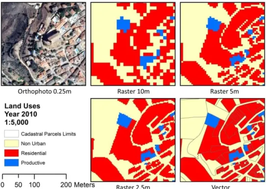
(7) processes, but the model’s capacity to reproduce urban growth processes is more limited when using more detailed scales such as those employed in urban planning (Stevens & Dragicevic, 2007), since urban structure is not composed of regular, equal cells but rather of a set of irregular-shaped structures or units. In fact, model outputs are sensitive to the cell size selected for representing urban space in raster surfaces, and the selection of one or another size can create differences in urban morphology. To explore this idea, several studies have been conducted on this relaxation of CA structure, most notably concerning the use of irregular cells based on: (i) Voronoi polygons for representing urban clusters (Semboloni, 2000), space object interactions (Shi & Pang, 2000) or other geographical objects (Hu & Li, 2004); (ii) Delaunay triangulation derived from plot centroids to model neighbourhood in an urban gentrification model (O'Sullivan, 2001 a, b); (iii) land use parcels to simulate changes (Stevens & Dragicevic, 2007); (iv) census blocks to simulate urban growth (Pinto & Antunes, 2010); (v), a set of irregular geographical objects that also enable changes in their structure (Moreno & Marceau, 2006; Moreno et al., 2008; Moreno et al., 2009); and (vi), cadastral parcels which define land property structure (Dahal & Chow, 2014). Given the greater realism in space representation that other alternatives offer, it seems appropriate to employ another kind of space representation that considers the irregularity of the land studied, rendering the model more realistic. 2.3. Relaxation of CA spatial structure: Towards a vector CA-based model. From among the possible relaxations presented above, it is the one related to space representation which may be most useful when simulating urban dynamics at a high level of detail, as mentioned earlier, although it has not been one of the most widely explored in CAbased modelling (see section 2.2). Of all the several possible irregular space structures, cadastral parcels represent the best solution for simulating urban growth more realistically and bringing the model closer to urban planning processes, since planners use the same representation. These parcels could be represented in a raster format but, as indicated above, this choice would not solve the problem as outputs are sensitive to cell size (Figure 2). Parcels were considered as the minimum spatial unit of the space within the model prototype described here, and they formed the structure with which the automata worked. Each parcel could contain different land uses, a given neighbourhood size and effect, transition rules could be applied, etc. Nevertheless, it was necessary to redefine some aspects typical of parametric CA-based models, especially neighbourhood, since a regular neighbourhood such as Moore or Von Neumann could not be applied in this case. It was also important to identify a computational solution that would enable the model to run within a reasonable length of time..

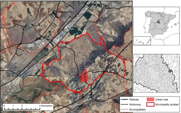
(8) Figure 2: Comparison of raster and vector parcels and land use representation.. 3. Methodology and materials. 3.1. Study area and input data. With more than 6.4 million inhabitants (INE, 2013), the Community of Madrid is one of the most dynamic spaces in the Iberian Peninsula, and in Europe in general, as regards land use change (Plata Rocha et al., 2009). These changes have involved massive land urbanisation as a result of the housing bubble at the beginning of the century. Within this Community, one of the most dynamic environments is the urban-industrial Henares Corridor located more than 50km from Madrid (capital of Spain) and the neighbouring city of Guadalajara. One of the municipalities inside this area has not yet experienced such massive urban growth and was therefore selected since there is still a chance of proposing more sustainable and balanced urban plans (Figure 3). Hence, Los Santos de la Humosa formed the ideal place for developing and testing tools that enable better urban growth management..

(9) Figure 3: Municipality of Los Santos de la Humosa employed to test the prototype.. In the case presented here, and within the Spanish legal framework, the changes and urban growth that a municipality will experience in future years are defined in the General Urban Land Use Plan (PGOU in Spanish). This plan is based on a cadastral parcel structure that subdivides the land in accordance with land uses and land property. In addition to building land and green belts, the future land uses envisaged for each parcel are also identified and drawn. Thus, parcels can be considered the 'canvas' on which future Spanish urban spaces are 'drawn', and they constitute a suitable spatial structure with which to model and simulate urban growth more realistically. This was therefore the structure used for discrete space representation in the prototype presented here. The input data (Table 1) comprised cadastral parcels, whose associated data and vector structure would be the medium on which the automata would act. Together with the cadastral data, municipal boundaries enabled us to define the extent of the municipality under study. Zoning status enabled identification of parcel status within the legal planning framework, recording the designated land use for each parcel and also any prohibition on locating given land uses in some of them. The road network layer was used to calculate accessibility and the suitability layer was used to determine the parcel's intrinsic capacity for development as urban land. Data layer. Cadastral Data. Scale/Resolution. 1:500 - 1:1,000. Format. Vector. Source. Description. General Directorate for Cadastre, Ministry of Finance and Public Administration, Government of Spain. Contains information at parcel level about: ID, municipality, use, year of construction, area, centroid, etc. The cadastral street map also includes the linear structure of the street axes..

(10) Municipal Limits. Zoning Status. Road Network. Suitability Map. 1:25,000. 1:50,000. 1:25,000. 50m. Vector. BCN25 - National Centre for Geographical Information, Directorate General of the National Geographic Institute, Ministry of Development, Government of Spain. Gives the geographical boundaries of each municipality.. Vector. Department of Environment, Housing and Land Use Planning, Community of Madrid. Classifies land according to its legal category: urban, non-building, building, etc., as well as the use for which it is destined.. Vector. BCN25 - National Centre for Geographical Information, Directorate General of the National Geographic Institute, Ministry of Development, Government of Spain. Network of national and regional roads.. Raster. Gómez- Delgado & EspinosaRodríguez (2012) – suitability map used for the Community of Madrid CA-based model.. Gives a value for each cell based on: height, slope, inhabitants and land use, among others.. Table 1: Data layers employed as input for the prototype.. 3.2. Conceptual basis of the prototype. As with most CA-based models, the prototype starts from an initial situation to which transition rules and factors are applied in order to simulate the possible future status of the urban space. The factors implemented in this prototype (neighbourhood, accessibility, suitability and zoning status) were based on those applied in the NASZ model schema (White et al., 1997), which has traditionally been employed in CA-based models to simulate urban growth. Cadastral parcels from 2010 formed the starting point. To test the prototype's operability, only two urban land uses were simulated: residential and productive (which include commercial and industrial areas) land uses, this latter including both commercial and industrial areas. Each iteration was equivalent to one natural year and land uses were updated with each iteration so that the land use changes obtained by the prototype during one iteration affected subsequent iterations. Five iterations were computed, to obtain the urban situation in 2015. Each factor implementation is explained below. NEIGHBOURHOOD Neighbourhood defines the geographical domain of influence (Tobler, 1979). It not only identifies which parcels (or cells in raster models) are neighbours, but also quantifies the effect of neighbouring land uses. This effect, also known as the push-and-pull effect, expresses the greater or lesser tendency for a land use to be developed in any given location according to neighbourhood. In this case, the vector structure of space offers a new means for determining neighbourhood. Due to the irregular structure, neighbourhood will vary according to parcel size and land use; thus, each parcel’s neighbourhood will differ from that of the others. In this version of the prototype, adjacent parcels were considered as neighbours, as were those partially or totally covered by the extent of a distance buffer from the studied parcel (neighbourhood a and b in.

(11) Figure 2 of Stevens & Dragicevic, 2007). The distance selected was 500m derived from a test that covered distance from 25m to 1000m, which in this case was sufficient due to municipality characteristics. The prototype would consider as neighbours, of the parcel being studied, those parcels that are totally or partially covered by the buffer of 500m. Once neighbouring parcels had been identified, the effect that each of them exerted on the studied parcel was calculated for each moment. If a parcel was being considered for development as new urban land, the push-and-pull effect that the other parcels exerted on it was calculated depending on their land use. For example, a parcel being considered for development as industrial land will receive a negative effect if the surrounding parcels contain a residential land use. In contrast, if industrial parcels are located nearby, this will positively attract this new use to the studied parcel. To calculate the effect of the neighbouring parcels, distance decay functions were employed. These functions are third degree equations that provide an attraction or repulsion value for a parcel according to its land use and the distance between it and the parcel being studied. In this case, these functions were derived from neighbourhood masks applied in the raster CA-based model presented in Gómez-Delgado and Rodríguez Espinosa (2012). These raster masks were applied over the entire CA grid and provided an attraction or repulsion value that varied over the distance to the central cell and the use it contained. Four distance decay functions were derived from these mask values and the distances, and applied in this prototype (Figure 4). These functions calculated: 1) the push-and-pull effect that productive parcels exert on vacant land for development as productive land, 2) the push-andpull effect that residential land exerts on vacant land for development as productive land, 3) the push-and-pull effect exerted by productive land on vacant land for development as residential land, and 4) the push-and-pull effect exerted by residential land on vacant land for development as residential land..

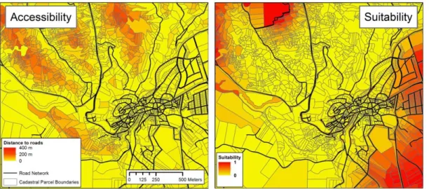
(12) Figure 4: Distance decay functions derived from raster masks. The raster mask conversion to function (1) is shown as an example. The same method is applied to (2), (3) and (4).. As it is shown in the following sections, neighbouring parcels in the prototype were identified using buffers and then abstracted to a graph, so that every parcel considered a neighbour of the parcel under study was linked to it using an edge in the graph. These edges stored values such as distance between parcels, land use of each parcel and the push-and-pull effect exerted. As the maximum neighbourhood distance was set at 500m, only a part of the functions shown in Figure 4 were used. ACCESSIBILITY One of the driving forces of urban change is proximity to a road network. Thus, industrial and commercial areas require efficient connections with a high capacity transport network. On the other hand, residential areas and urban centres require multiple access routes, not only based on proximity to the road network but also on connectivity between roads. Using the national road network map and the cadastral layers that store roads within urban areas (Table 1), a new road network layer was generated for the studied area. An accessibility value was computed for each parcel (Figure 5a) as the shortest distance to the road network. This enabled identification of parcels with an optimum spatial situation and road network access. SUITABILITY Suitability is defined as the intrinsic capacity of a specific area to contain one land use or another. Several variables are often included in this parameter, such as height, slope or kind of soil, which together define a parcel's capacity for developing a new land use. Thus, this parameter should include all the relevant variables that render an area more or less ideal for containing a new land use. Due to the goal of this study, we used a previously developed suitability map (Table 1). It has been obtained through a spatial logistic regression, obtaining the coefficients for each variable that explain urban growth between 1990 and 2000: population increase, elevation, slope, distance to water bodies or existing land uses (Gómez-Delgado & Espinosa-Rodríguez, 2012). This suitability map enabled us to obtain a suitability value at the parcel level, but due to its raster nature it was necessary to process this information in order to combine it with the cadastral parcels. Consequently, we performed a spatial intersection between the suitability map and the parcels so that a mean suitability value could be assigned to each parcel (Figure 5b). This value was directly proportional to the surface that each raster cell from the map occupied within the parcel being studied..

(13) Figure 5: Accessibility (a) and Suitability (b) values at the parcel level.. ZONING STATUS Neighbourhood, accessibility and suitability are related to the geographical and physical characteristics of the parcels, whereas zoning status is related to their legal characteristics. Zoning status determines the legal status of a parcel within the Spanish legal framework, indicating if the parcel is within an urban area, and is building land or non-building land. Each municipality in Spain defines the status of each parcel in their General Urban Land Use Plan (PGOU). In this case, a zoning status map at the level of the Community of Madrid for the year 2008 (Figure 6) was employed (which was sufficient bearing in mind that urban plans in Spain present little changes over time once they have been approved). As with the suitability map, we carried out a spatial intersection between the cadastral layer and the map, assigning the classification to each parcel. These values worked as a mask within the prototype, excluding parcels that were not suitable for urban development from the calculation in each iteration.. Figure 6: Zoning status of the studied area.. TRANSITION POTENTIAL.

(14) Each of the four factors described above provides a value at the parcel level. CA-based models that simulate urban growth have traditionally applied a parametric equation in order to compute the transition potential of each cell. This value indicates the extent to which a parcel is more or less prone to develop an urban land use based on its neighbourhood, accessibility, suitability and zoning status. It is also common to add a stochastic parameter in order to reproduce the uncertainty related to urban and social processes (Ménard & Marceau, 2005). However, this stochastic or random parameter was not included in the present prototype because the aim was solely to determine the viability of a vector prototype and the use of graphs as a computational solution. The present prototype employs a similar equation (equation 1) which includes the four previously mentioned factors based on the NASZ model schema proposed by White et al. (1997). 𝑛. 𝑃𝑖,𝑘 = (∑ 𝑁𝑖,𝑗 ) 𝐴𝑖 𝑆𝑖 𝑍𝑖 𝑗=1. Equation 1: Transition potential to a land use 'k' for a parcel 'i'.. Neighbourhood N, Accessibility A, Suitability S and Zoning Status Z values are multiplied in order to obtain a transition potential value for each parcel. The neighbourhood value includes the sum of the effect that the set of neighbours exerts on parcel 'i'. Once the potential has been calculated for residential and productive land use, the prototype determines which parcels will be developed in each iteration. These new urban parcels are then added to the existent urban parcels, and the transition potential value is recalculated in the following iterations based on the new situation. 3.3. Spatial structure transformation using graph theory. The disadvantage of representing land as an irregular structure is that it entails a substantial increase in computational time as a result of the vector structure employed and associated operations. In this case, if the level of detail or the number of parcels to be processed is not high, the CA could be executed within a specific GIS tool or through an ad hoc model implementation in a programming language. In contrast, if the number of parcels is so high that it impedes fast running of the model, it will be necessary to find other ways of processing. A good approach to solve this problem is to abstract the vector representation to a graph-type format (O'Sullivan, 2001b). A graph can be defined as in equation 2, where graph 'G' is composed of a set of nodes 'V' and a set of edges or links 'E' that connect two elements of 'V' (Jantz et al., 2010). 𝐺 = (𝑉, 𝐸); where E  [V2] Equation 2: Graph 'G' definition.. The most usual way to represent a graph is through a drawing where each entity is represented as a node and the relations between them are expressed as links or edges, connecting pairs of nodes (Figure 7)..

(15) Figure 7: Usual representation of a graph. Numbers within blue circles are the node identifiers and 'e' expresses the connection (edge) between nodes.. Graphs have been widely used to solve several kind of problems, many of them of a spatial nature, such as shortest path calculation (Goldberg & Harrelson, 2005), optimal paths (Xia, 2003) or transport network management (Anez et al., 1996), among others. They have also been employed to represent urban phenomena such as urban gentrification (O'Sullivan, 2001b), where each building was expressed as a node and the adjacent buildings were represented as neighbours by means of edges. In the case of urban simulation models, the use of graphs has already been tested in raster surfaces (Sarkar et al., 2009). In the case presented here, the vector structure in which the CA runs is abstracted to a graph representation, where each parcel is represented as a node and the edges connect parcels (nodes) considered as neighbours (Figure 8). Thus, the need to read the vector structure of the cadastral parcel in each iteration is avoided and the topology is conserved through the graph. Each node and each edge store all the information necessary for the model to run, for example: parcel identifier, land use contained, year of development, parcel suitability, accessibility value, zoning status, neighbouring parcels, effect of neighbouring parcels, etc.. Figure 8: Perspective view of part of the studied area with orthophoto, cadastral parcels and graph abstraction..

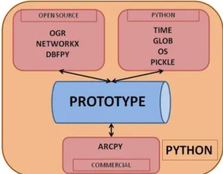
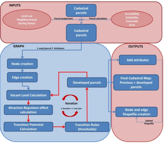
(16) In addition, neighbourhood is expressed through the edges in the graph, storing the distance between the connected parcels, their land uses and the push-and-pull effect that they exert. For example, if a parcel 'A' has 'B', 'C' and 'D' as neighbours, one unique edge will be created for each neighbour (AB, AC, AD). 3.4. Prototype implementation. We opted to design and implement the prototype directly in a programming language in order to obtain greater flexibility and avoid software restrictions (Batty et al., 1999; White et al., 1997). Python (Van Rossum & Drake Jr., 2008) is the programming language used nowadays in several programmes to develop their tools, especially those that work with geospatial data, whether they are commercial or open source. Our prototype was implemented using this language, combining commercial libraries such as ArcPy from ArcGIS and open-source libraries such as OGR from GDAL (Fundation, 2008) to manage spatial data, or a specific library to create and manage graphs called Networkx (Hagberg et al., 2008), besides the other libraries and functions typical of Python (Figure 9).. Figure 9: Python, open source and commercial libraries used for the prototype.. The prototype runs through a set of functions especially designed for this purpose that combine some of the libraries shown in Figure 9. These functions are stored in a Python script where each function is independent from the others and they work as another library in the eyes of the user. This independence enables perfect identification of the point where the prototype is during each run and more rapid isolation of the problems that could appear. FLOWCHART Figure 10 shows a flowchart of the current version of the prototype, summarising the entire process from the input data to the final output..

(17) Figure 10: Flowchart of the prototype.. First, functions are run to process the input data (cadastral parcels and their information) so that the prototype has all the data and parameters required to start running. Second, a graph is created by abstracting the vector representation making use of the Networkx library, generating one node per parcel which stores all the information related to each parcel (identifier, land use, suitability value, neighbouring parcels, etc.). Once the graph nodes have been created, the edges between neighbouring nodes must be established. To do this, for each parcel the attribute table stores the identifier of neighbouring parcels (those that are partially or completely at a 500m distance from the studied parcel). An edge between the studied parcel and each of its neighbouring parcels is created, which stores the distance and land uses of the parcels involved. Once the graph is ready, the transition rules process starts running so that the developing parcels can be calculated. A list is obtained of the parcels classified as building land (vacant land that can be developed as urban within the local urban plan). With this vacant parcels list, the pushand-pull effect that neighbouring parcels exert on each of them is calculated using the distance decay functions presented in section 3.2. Two values are obtained for each parcel: neighbourhood effect on developing a residential land use in the parcel and the effect on developing a productive land use. These values are the direct sum of all the values that each parcel exerts on the studied parcel..

(18) Once those parcels suitable for developing urban land use have been identified and the neighbourhood effect has been calculated, it is time to apply the transition rules. These rules are applied by means of the transition potential calculation, and they are established according to the parameters involved: accessibility, suitability, neighbourhood and also the zoning status that at this point has acted as a mask when selecting the vacant parcels. The parcels that are going to be developed are obtained according to the first three parameters calculated for each parcel and using the threshold area previously established for each land use. Then, the first iteration of the prototype is run, which is equivalent to one natural year. For the rest of the iterations, the vacant parcels list is obtained first, then the push-and-pull effect between parcels is recalculated according to the new situation (changes derived from the previous iteration), and finally, the transition rules are applied. This process is repeated for the rest of the iterations that are programmed in the prototype. Once the final iteration has finished (2015), the modelling process is stopped, converting the results derived from the graph into a spatial vector representation in three main steps: 1) converting the results from the graph into a cadastral parcel attributes table, which stores the new urban growth; 2) creating a node and edge vector file; and 3) completing the node and edge attributes table with the results derived from the graph. 4. Results. Outputs derived from the graph are translated into the vector file containing the cadastral parcels, updating their attributes once all iterations have finished. The final cadastral map is shown in Figure 11, highlighting the new urban growth: developed residential parcels and developed productive parcels. The prototype started in year 2010 and 5 iterations were computed, so the figure shows the situation in 2015.. Figure 11: Output derived from the graph. New urban land uses in 2015 are highlighted.. As the objective was simply to test the viability of the prototype, further analysis of the results is unnecessary. The capacity of the model has been tested, and it ran within a reasonable computational time: less than 15 minutes on an Intel® Core™ i7-4790 (3.6 GHz, 8 MB cache, 4.

(19) cores) PC with 16 GB of RAM. The great part of the time is spent in the definition of the edges of the graph which are more than 3 million with over 4,000 nodes. The rest of the time, which would be the application of the transition rules is less than 10 seconds per iteration (which represent a natural year). As shown in Figure 11, new residential areas were located in two separate spaces: one in the north and the other in the south of the study area, both enabling aggregated growth. New productive areas were located in the surroundings of the urban centre due to the push-and-pull effect exerted by other residential and productive areas, and also due to the effect of accessibility. 5. Discussion 5.1. Contribution of the prototype The main objectives of the present study was: (1) to explore the viability of implementing a new model (in this case a prototype) that combines the basic characteristics of a classical CA with new space representation techniques (vector) and (2) to find a computational solution such as graph theory to deal with vector structures. The prototype still requires further improvement in order to analyse the results in greater depth (calibration, validation and future simulation) and eventually yield a complete CA-based urban growth model. The problem of identifying a more realistic mean of space representation appears to have been almost solved by the use of cadastral parcels and their abstraction to a graph. As was previously mentioned, in Spain, responsibility for local urban planning development is devolved to the municipalities (approval for such development is the responsibility of the community in which it is envisaged) and cadastral parcels are the elements used to structure land and they are also the minimum unit employed by developers to design urban plans. The goal of developing simulation models such as the prototype presented here is to achieve models that more closely reflect urban planning processes in order to offer different growth alternatives for planners to assess, and thus facilitate better decision-making (Triantakonstantis & Mountrakis, 2012). The use of a space representation based on the reality of urban planning would definitely lead to a better urban growth modelling process, since there would be a better understanding between modellers and decision makers. Other kinds of representation could have been employed, such as geographical objects or census blocks (Moreno et al., 2008; Pinto & Antunes, 2010), but in the specific case of Spain we think that the use of cadastral parcels is the best choice. Although cadastral parcels may be a good option, they also present some limitations. In this sense, the prototype can only simulate whether a whole parcel is going to be developed or not. Rural parcels, which are usually larger than urban plots, are often divided into smaller parcels or sub parcels, leading to the development of a little part of them. The prototype has not already a split-up algorithm that subdivides large parcels into smaller ones, but it should be solved in the future full working model. Regarding implementation of the prototype, vector representation involves higher computational time costs so it was necessary to find a way to overcome this limitation. Abstraction of vector representation to a graph (based on O’Sullivan, 2001b) simplifies the computational problem, in which the highest cost is related to edge creation compared with the rest of the operations. At every moment of the graph run, each parcel is perfectly identified as a node with its entire set of attributes. Neighbourhood definition is also more efficient due to the.

(20) clear and immediate identification of each parcel’s neighbours. Therefore, the main objective of this work is achieved. Furthermore, full implementation of the prototype using pure code yielded greater flexibility, making it possible to edit each programming block independently of the others. The usefulness of this approach resides in the possibility of obtaining a dynamic model (Batty et al., 1999) rather than a static one, in a GIS software package. The use of Python, one of the most widespread programming languages in geospatial data management and analysis, enabled us to combine the advantages of commercial library tools with those in open-source libraries. Other authors have suggested that it is necessary to choose one or the other, but in this case we saw this combination as an opportunity rather than a problem since we could decide what to use in each moment. The code used in the modelling step could be optimised further, and more work is required to improve its efficiency. The prototype, in this stage, is able to run several iterations and to provide the allocation for future urban development under the premises of the parameters implemented as it was shown in Figure 11. In this work, the computational and operational viability of the prototype has been tested, but, future research should cover a full calibration and a validation process that provide a correspondence between real and simulated urban growth, in order to pass from a prototype to a full working model. In this sense, we could perform the calibration process making use of some of the methods available in the literature (e.g. Barreira et al., 2015; Goldstein, 2004). 5.2. Development of the parameters The aim of the prototype was not only to solve the problem of defining neighbourhood, but also to explore the viability of implementing the push-and-pull effect between land uses by means of edges. The flexibility of the graph provides the possibility of calculating the effect that one parcel (node) exerts on another and vice versa. However, this approach to modelling this effect could be questioned, and it is therefore necessary to conduct further studies on how these processes occur in reality, paying more attention to how actual land use distribution influences the allocation of new land uses. Although we used a 500m neighbourhood distance for this study area, this distance could be increased or decreased when modelling other urban areas, and it could also be modelled as a dynamic distance (Moreno et al., 2009). A limitation of the current push-and-pull effect algorithm is that, for example, parcels that only a little part of themselves are in the 500m buffer, are considered also as neighbours of the studied parcel so it might not be appropriate. It would be interesting to model the push-and-pull effect taking into account the specific amount of area within the buffer of each neighbouring parcel. By representing space as cadastral parcels, we avoided the problem of cell size influencing our results (Jantz & Goetz, 2005; Ménard & Marceau, 2005) or neighbourhood definition using multi-grids (Van Vliet et al., 2009). In this case, our results might be sensitive to the resolution of the input layers, to the selected distance and to how neighbours are identified, so we could also explore how other neighbourhood definitions might affect the results (Dahal & Chow, 2015). In relation to accessibility, although it was calculated as the shortest Euclidean distance between the parcel centroids and the road network, this could be improved by the incorporation of a weighted value related to the type of road. In order to calibrate the model for a given past time period, there might be some roads or motorways that could be developed within that period, so the introduction of new road links could drive the model towards different results (Barredo et al..

(21) 2003). Another approach that might improve the model would be to include the road network as a subgraph within the cadastral graph, to compute calculations by means of the network and obtain accessibility values as in transport models (de Dios and Willumsen, 2011). The transition rules applied were entirely prescriptive in this first version of the prototype, applying thresholds that permitted decisions about whether a parcel would be developed or not. Thus, a complete calibration that adjusts the thresholds and the entire set of parameters is required, especially for neighbourhood (Van Vliet et al., 2013). Once the prototype has been calibrated, it would be capable of simulating a tendency in a past period and reproducing it in the present for validation. The methodology proposed here does not include a random factor that reproduces the uncertainty related to urban growth, where human decisions play a key role (García et al., 2011). Thus, it would seem necessary to include some kind of randomness. 6. Conclusions. The present study has demonstrated the viability of using a vector representation of space in CA-based urban growth modelling when combined with graph theory. The use of cadastral parcels as the automata cell could bring these tools closer to the reality faced by urban planners and people responsible for decision-making, by working at the same scale as local urban plans. Graph theory shows great potential to operate with vector spaces. Here, the capacity of a graph to build non-static neighbourhoods has been tested and shown to work within a reasonable computational time. A 500m neighbourhood buffer was employed, but it would be useful to model irregular buffer sizes according to the area of the parcel being studied, to the land use contained or the desired urban pattern. Each of the required parameters was added at the parcel level, so the related data was stored within the graph. No randomness was included, but could evidently be added in several parts of the prototype. The results derived from graph calculations can be easily translated to the cadastral structure for visualisation and analysis. Demand was introduced as an area development rate per iteration, so complete parcels were developed at the end of each iteration. Since not every land use change takes the same time to occur, a percentage of area development at parcel level could be introduced. Further work is required on calibration in order to obtain a full working model since the present prototype was only used to test the operational viability of using cadastral parcels and graph theory to model urban growth. Future research should also cover a validation process that would enable the. model to simulate different approaches and scenarios in order to make better decisions in urban planning. ACKNOWLEDGEMENTS. This research was performed within the context of SIMURBAN2 project (Geosimulation and environmental planning on metropolitan spatial decision making. Implementation to intermediate scales) (CSO2012-38158-C02-01), funded by the Spanish Ministry of Economy and Competitiveness. The Universidad de Alcalá supports the first author within the “Ayudas para la Formación de Personal Investigador (FPI) 2012” framework. The authors would also like to thank the “Servicio de Traducción de la Universidad de Alcalá” which provided language help. Finally, the authors would like to thank the anonymous reviewers by their comments and proposals made..

(22) BIBLIOGRAPHY Aguilera, F., Valenzuela, L. M., & Bosque, J. (2010). Simulación de escenarios futuros en la aglomeración urbana de granada a través de modelos basados en autómatas celulares. Boletín De La Asociación De Geógrafos Españoles, 54, pp. 271-300. Aguilera, F., Valenzuela, L. M., & Botequilha-Leitao, A. (2011). Landscape metrics in the analysis of urban land use patterns: A case study in a Spanish metropolitan area. Landscape and Urban Planning, 99 (3-4), pp. 226-238. Alberti, M., & Marzluff, J. M. (2004). Ecological resilience in urban ecosystems: linking urban patterns to human and ecological functions. Urban ecosystems, 7, pp. 241-265. Aljoufie, M., Zuidgeest, M., Brussel, M., van Vliet, J., & van Maarseveen, M. (2013). A cellular automata-based land use and transport interaction model applied to Jeddah, Saudi Arabia. Landscape and Urban Planning, 112, pp. 89-99. Anez, J., De La Barra, T., & Perez, B. (1996). Dual graph representation of transport networks. Transportation Research Part B: Methodological, 30, pp. 209-216. Baetens, J. M., Van der Weeën, P., & De Baets, B. (2012). Effect of asynchronous updating on the stability of cellular automata. Chaos, Solitons & Fractals, 45(4), 383-394. Bardají, E. (2011). El planeamiento de escala intermedia como corazón del planeamiento español: una propuesta de nueva organización de las figuras de planeamiento. Ciudad y territorio: Estudios territoriales, XLIII CUARTA ÉPOCA, pp. 579-585. Barredo, J. I., Demichelli, L., Lavalle, C., Kasanko, M., & McCormick, N. (2004). Modelling future urban scenarios in developing countries: an application case study in Lagos, Nigeria. Environment and Planning B: Planning and Design, 31 (1), pp. 65-84. Barredo, J. I., Kasanko, M., McCormick, N., & Lavalle, C. (2003). Modelling dynamic spatial processes: simulation or urban future scenarios through cellular automata. Landscape and Urban Planning, 64, pp. 145-160. Barredo, J. I., & Gómez-Delgado, M. (2008). Towards a set of IPCC SRES urban land use scenarios: modelling urban land use in the Madrid region. In Modelling Environmental Dynamics (pp. 363-385). Springer Berlin Heidelberg. Barreira González, P., Aguilera-Benavente, F., & Gómez-Delgado, M. (2015). Partial validation of cellular automata based model simulations of urban growth: An approach to assessing factor influence using spatial methods. Environmental Modelling & Software, 69, pp. 77-89. Batty, M. (1998). Urban evolution on the desktop: simulation with the use of extended cellular automata. Environment and Planning A, 30, pp. 1943-1967. Batty, M. (2007). Cities and complexity: understanding cities with cellular automata, agentbased models, and fractals. The MIT press. Batty, M., Xie, Y., & Sun, Z. (1999). Modeling urban dynamics through GIS-based cellular automata. Computers, Environment and Urban Systems, 23, pp. 205-233..

(23) Benenson, I., & Torrens, P. M. (2004). Geosimulation : automata-based modelling of urban phenomena. Hoboken, NJ: John Wiley & Sons. Berling-Wolff, S., & Wu, J. (2004). Modelling urban landscape dynamics: A review. Ecological Research, 19, pp. 119-129. Cornforth, D., Green, D. G., & Newth, D. (2005). Ordered asynchronous processes in multiagent systems. Physica D: Nonlinear Phenomena, 204, pp. 70-82. Couclelis, H. (1985). Cellular worlds: a framework for modeling micro-macro dynamics. Environment and Planning A, 17, pp. 585-596. Couclelis, H. (1997). From cellular automata to urban models: new principles for model development and implementation. Environment and Planning B: Planning & Design, 24, pp. 165-174. Dahal, K. R., & Chow, T. E. (2014). An agent-integrated irregular automata model of urban land-use dynamics. International Journal of Geographical Information Science, 28, pp. 22812303. Dahal, K. R., & Chow, T. E. (2015). Characterization of neighborhood sensitivity of an irregular cellular automata model of urban growth. International Journal of Geographical Information Science, 29, pp. 1-23. de Almeida, C. M., Batty, M., Vieira Monteiro, A. M., Câmara, G., Soares-Filho, B. S., Cerqueira, G. C., & Pennachin, C. L. (2003). Stochastic cellular automata modeling of urban land use dynamics: empirical development and estimation. Computers, Environment and Urban Systems, 27(5), pp. 481-509. de Dios Ortúzar, J., & Willumsen, L. G. (2011). Modelling transport. John Wiley & Sons. Dietzel, C., & Clarke, K. C. (2004). Spatial Differences in Multi‐Resolution Urban Automata Modeling. Transactions in GIS, 8, pp. 479-492. Engelen, G., White, R., Uljee, I., & Drazan, P. (1995). Using Cellular-Automata for Integrated Modeling of Socio-Environmental Systems. Environmental Monitoring and Assessment, 34, pp.203-214. Engelen, G., Lavalle, C., Barredo, J. I., Van der Meulen, M., & White, R. (2007). The MOLAND modelling framework for urban and regional land-use dynamics. In Koomen, E., & Stillwell, J. (2007). Modelling land-use change. Springer Netherlands (pp. 297-320). Frankhauser, P. (1998). Fractal geometry of urban patterns and their morphogenesis. Discrete dynamics in Nature and Society, 2, pp. 127-145. Fundation, O. S. G. (2008). GDAL-OGR: Geospatial Data Abstraction Library/Simple Features Library Software. Garcia, A. M., Sante, I., Crecente, R., & Miranda, D. (2011). An analysis of the effect of the stochastic component of urban cellular automata models. Computers Environment and Urban Systems, 35, pp. 289-296..

(24) Gardner, M. (1970). Mathematical games: The fantastic combinations of John Conway’s new solitaire game “life”. Scientific American, 223, pp. 120-123. Goldberg, A. V., & Harrelson, C. (2005). Computing the shortest path: A search meets graph theory. Proceedings of the sixteenth annual ACM-SIAM symposium on Discrete algorithms. Society for Industrial and Applied Mathematics. pp. 156-165. Goldstein, N. C. (2004). Brains versus brawn—comparative strategies for the calibration of a cellular automata-based urban growth model. In Atkinson, P., Foody, G. M., Darby, S. E., & Wu, F. (Eds.). (2004). GeoDynamics. CRC Press. (pp. 249-272). Gómez-Delgado, M., & Rodríguez-Espinosa, V. M. (2012). Análisis de la dinámica urbana y simulación de escenarios de desarrollo futuro con tecnologías de la información geográfica. (p. 352). RA-MA EDITORIAL. Hagberg, A., Swart, P., & S Chult, D. (2008). Exploring network structure, dynamics, and function using NetworkX. Los Alamos National Laboratory (LANL). Hewitt, R., Van Delden, H., & Escobar, F. (2014). Participatory land use modelling, pathways to an integrated approach. Environmental Modelling & Software, 52, pp. 149-165. Hu Shiyuan & Li Deren (2004). Vector cellular automata based geographical entity. 12th Int. Conf on Geoinformatics - Geospatial Information Research: Brindging the Pacific and Atlantic University of Gävle, Sweden. pp. 249-256. INE (2013). Instituto Nacional de Estadística. Madrid. Itami, R. M. (1994). Simulating spatial dynamics: cellular automata theory. Landscape and Urban Planning, 30, pp. 27-47. Jantz, C. A., & Goetz, S. J. (2005). Analysis of scale dependencies in an urban land-use-change model. International Journal of Geographical Information Science, 19, pp. 217-241. Jantz, C. A., Goetz, S. J., Donato, D., & Claggett, P. (2010). Designing and implementing a regional urban modeling system using the SLEUTH cellular urban model. Computers, Environment and Urban Systems, 34, pp. 1-16. Jokar Arsanjani, J., Helbich, M., Kainz, W., & Darvishi Boloorani, A. (2013). Integration of logistic regression, Markov chain and cellular automata models to simulate urban expansion. International Journal of Applied Earth Observation and Geoinformation, 21, pp. 265-275. Kasanko, M., Barredo Cano, J. I., Lavalle, C., McCormick, N., Demichelli, L., Sagris, V., & Brezger, A. (2006). Are European cities becoming dispersed? A comparative analysis of 15 european urban areas. Landscape and Urban Planning, 77(1-2), pp. 111-130. Kocabas, V., & Dragicevic, S. (2006). Assessing cellular automata model behaviour using a sensitivity analysis approach. Computers, Environment and Urban Systems, 30(6), pp. 921-953. Lauf, S., Haase, D., Hostert, P., Lakes, T., & Kleinschmit, B. (2012). Uncovering land-use dynamics driven by human decision-making–A combined model approach using cellular automata and system dynamics. Environmental Modelling & Software, 27, pp. 71-82..

(25) Leao, S., Bishop, I., & Evans, D. (2004). Simulating urban growth in a developing nation's region using a cellular automata-based model. Journal of Urban Planning and DevelopmentAsce, 130, pp. 145-158. Lee, J., Adachi, S., Peper, F., & Morita, K. (2004). Asynchronous game of life. Physica D: Nonlinear Phenomena, 194, pp. 369-384. Li, X., Yang, Q. S., & Liu, X. P. (2008). Discovering and evaluating urban signatures for simulating compact development using cellular automata. Landscape and Urban Planning, 86, pp. 177-186. Liu, X. H., & Andersson, C. (2004). Assessing the impact of temporal dynamics on land-use change modeling. Computers, Environment and Urban Systems, 28, pp. 107-124. Liu, Y. (2012). Modelling sustainable urban growth in a rapidly urbanising region using a fuzzy-constrained cellular automata approach. International Journal of Geographical Information Science, 26, pp. 151-167. Macgill, S. M. (1986). Research Policy and Review .12. Evaluating a Heritage of Modeling Styles. Environment and Planning A, 18, pp. 1423-1446. Ménard, A., & Marceau, D. J. (2005). Exploration of spatial scale sensitivity in geographic cellular automata. Environment and Planning B: Planning and Design, 32(5), pp. 693-714. Mitsova, D., Shuster, W., & Wang, X. H. (2011). A cellular automata model of land cover change to integrate urban growth with open space conservation. Landscape and Urban Planning, 99, pp. 141-153. Moreno, N., & Marceau, D. (2006). A vector-based cellular automata model to allow changes of polygon shape. In International Conference on Modeling and Simulation-Methodology, Tools, Software Applications, Calgary, Canada. Moreno, N., Ménard, A., & Marceau, D. J. (2008). VecGCA: a vector-based geographic cellular automata model allowing geometric transformations of objects. Environment and Planning BPlanning & Design, 35, pp. 647-665. Moreno, N., Wang, F., & Marceau, D. J. (2009). Implementation of a dynamic neighborhood in a land-use vector-based cellular automata. Computers Environment and Urban Systems, 33, pp. 44-54. O'Sullivan, D. (2001a). Exploring spatial process dynamics using irregular cellular automaton models. Geographical Analysis, 33, pp. 1-18. O'Sullivan, D. (2001b). Graph-cellular automata: a generalised discrete urban and regional model. Environment and Planning B: Planning & Design, 28, pp. 687-706. O´Sullivan, D., & Torrens, P. (2000). Cellular Models of Urban Systems. CASA Working Paper Series. London: Centre for Advanced Spatial Analysis (University College London). Pinto, N. N., & Antunes, A. P. (2010). A cellular automata model based on irregular cells: application to small urban areas. Environment and Planning B-Planning & Design, 37, pp. 1095-1114..

(26) Plata Rocha, W., Gómez Delgado, M., & Bosque Sendra, J. (2009). Cambios de usos del suelo y expansión urbana en la Comunidad de Madrid (1990-2000). Scripta Nova: revista electrónica de geografía y ciencias sociales, 293(vol. 13), pp. 27. Portugali, J. (2000). Self-organization and the city. Springer. Samat, N. (2006). Characterizing the scale sensitivity of the cellular automata simulated urban growth: a case study of Seberan Perai Region, Penang State, Malaysia. Computers, Environment and Urban Systems, 30(6), pp. 905-920. Sante, I., Garcia, A. M., Miranda, D., & Crecente, R. (2010). Cellular automata models for the simulation of real-world urban processes: A review and analysis. Landscape and Urban Planning, 96, pp. 108-122. Sarkar, S., Crews-Meyer, K., Young, K., Kelley, C., & Moffett, A. (2009). A dynamic graph automata approach to modeling landscape change in the Andes and the Amazon. Environment and planning. B, Planning & Design, 36, pp. 300-318. Schönfisch, B., & de Roos, A. (1999). Synchronous and asynchronous updating in cellular automata. BioSystems, 51(3), 123-143. Semboloni, F. (2000). The growth of an urban cluster into a dynamic self-modifying spatial pattern. Environment and planning. B, Planning & Design, 27, pp. 549-564. Seto, K. C., Fragkias, M., Güneralp, B., & Reilly, M. K. (2011). A meta-analysis of global urban land expansion. PloS one, 6(8), e23777. Shafizadeh Moghadam, H., & Helbich, M. (2013). Spatiotemporal urbanization processes in the megacity of Mumbai, India: A Markov chains-cellular automata urban growth model. Applied Geography, 40, pp. 140-149. Shi, W. Z., & Pang, M. Y. C. (2000). Development of Voronoi-based cellular automata - an integrated dynamic model for Geographical Information Systems. International Journal of Geographical Information Science, 14, pp. 455-474. Silva, E. A., & Clarke, K. C. (2002). Calibration of the SLEUTH urban growth model for Lisbon and Porto, Portugal. Computers, Environment and Urban Systems, 26(6), pp. 525-552. Stevens, D., & Dragicevic, S. (2007). A GIS-based irregular cellular automata model of landuse change. Environment and Planning B-Planning & Design, 34, pp. 708-724. Stevens, D., Dragicevic, S., & Rothley, K. (2007). iCity: A GIS-CA modelling tool for urban planning and decision making. Environmental Modelling & Software, 22(6), pp. 761-773. Tobler, W. (1979). Cellular geography. Philosophy in geography. Springer. pp. 379-386 Tobler, W. R. (1970). Computer Movie Simulating Urban Growth in Detroit Region. Economic Geography, 46, pp. 234-240. Torrens, P. (2000). How cellular models of urban systems work. CASA Working Serie Papers. Centre for Advanced Spatial Analysis (University College London)..

(27) Torrens, P. M., & O'Sullivan, D. (2001). Cellular automata and urban simulation: where do we go from here? Environment and Planning B: Planning & Design, 28, pp. 163-168. Triantakonstantis, D., & Mountrakis, G. (2012). Urban Growth Prediction: A Review of Computational Models and Human Perceptions. Journal of Geographic Information System, 4, pp. 555-587. Turing, A. M. (1936). On computable numbers, with an application to the Entscheidungsproblem. Journal of Math, 58, pp. 345-363. Van Rossum, G., & Drake Jr, F. L. (2008). Python Tutorial. Python Software Foundation. URL: https://docs.python.org/2/. van Vliet, J., Naus, N., van Lammeren, R. J., Bregt, A. K., Hurkens, J., & van Delden, H. (2013). Measuring the neighbourhood effect to calibrate land use models. Computers, Environment and Urban Systems, 41, pp. 55-64. van Vliet, J., White, R., & Dragicevic, S. (2009). Modeling urban growth using a variable grid cellular automaton. Computers Environment and Urban Systems, 33, pp. 35-43. Verburg, P. H., Schot, P. P., Dijst, M. J., & Veldkamp, A. (2004). Land use change modelling: current practice and research priorities. GeoJournal, 61, pp. 309-324. White, R. (1998). Cities and cellular automata. Discrete dynamics in Nature and Society, 2, pp. 111-125. White, R., & Engelen, G. (1993). Cellular-Automata and Fractal Urban Form - a Cellular Modeling Approach to the Evolution of Urban Land-Use Patterns. Environment and Planning A, 25, pp. 1175-1199. White, R., & Engelen, G. (1997). Cellular automata as the basis of integrated dynamic regional modelling. Environment and Planning B: Planning & Design, 24, pp. 235-246. White, R., & Engelen, G. (2000). High-resolution integrated modelling of the spatial dynamics of urban and regional systems. Computers, Environment and Urban Systems, 24, pp. 383-400. White, R., Engelen, G., & Uljee, I. (1997). The use of constrained cellular automata for highresolution modelling of urban land-use dynamics. Environment and Planning B: Planning & Design, 24, pp.323-343. Wolfram, S. (1984). Cellular Automata as Models of Complexity. Nature, 311, pp. 419-424. Wu, D., Liu, J., Zhang, G., Ding, W., Wang, W., & Wang, R. (2009). Incorporating spatial autocorrelation into cellular automata model: An application to the dynamics of Chinese tamarisk (Tamarix chinensis Lour). Ecological Modelling, 220, pp. 3490-3498. Wu, F. (2002). Calibration of stochastic cellular automata: the application to rural-urban land conversions. International Journal of Geographical Information Science, 16, pp. 795-818. Xia, Q. (2003). Optimal paths related to transport problems. Communications in Contemporary Mathematics, 5, pp. 251-279..

(28) Zhang, Q., Ban, Y., Liu, J., & Hu, Y. (2011). Simulation and analysis of urban growth scenarios for the Greater Shanghai Area, China. Computers, Environment and Urban Systems, 35, pp. 126-139..

(29)