Geometric Differential Operators for Shape Modelling

(a) (b)

(c) (d) (e)

(f) (g) (h)

Figure 5.22: Uncompleted contours.

corrupted with gaussian noise (fig.5.20(a)) and a character ’S’ with uniform noise added (fig.5.20(c)). Meanwhile the set of real images is displayed in fig.5.21.

(a) (b) (c)

(d) (e) (f)

Figure 5.23: Extensions of brain (a), horse (b), hand (c), ’S’ (d), head (e) and fingerprint (f).

real images of fig.5.21(a)-(e), we used edges in combination with pixel gray level in the brain image and for the fingerprint in fig.5.21(f), image ridges. The contours obtained, shown in fig.5.22, include cases deserving special care, such as corner restoration (horse ears in fig.5.22(d), (g) and finger joints in fig.5.22(f)) and dense lines prone to merge (fingerprint in fig.5.22(h)).

The numeric scheme used to compute solutions to (4.3) is an explicit Euler scheme for non-linear heat equations stabilize by means of the stop criterion critB given in Section 5.1.1. The parameters used in the computation of the coherence vector fields are an integration scaleρ= 2 and a regularization scaleσ= 0.5. In the case of large gaps (fig.5.22 (e), (g)) vector fields are dynamically updated every 300 iterations. We have used the ridgeness measure described in [45] to compute the ridges of the extension that yield the curve closure and serve to update vector fields. According to the theoretic analysis given in Section 4.2.1, distance based vector fields properly recover a model of corners and linear fields avoid merging in the contours to complete. Therefore, for the sake of a maximum accuracy and reliability in the closed models, we have chosen the distance based DVF for restoration of contours in fig.5.22(a)-(h) and a linear LVF closing in the case of the fingerprint (fig.5.22(i)).

recon-(a) (b)

(c) (d) (e)

(f) (g) (h)

Figure 5.24: Reconstructed contours using DVF (a)-(g) and LVF (h).

were extracted via a morphological thinning of a thresholded version of the extensions. Because it is based on the distance map to the open contours, closings achieved using DVF recover shape curvatures, such as the concave part of the non-convex contour in fig.5.24(c) and the character ’S’ in fig.5.24(e). Besides it properly closes the acute angles of the horses ears (fig.5.24(d), (g)) and the hand finger joints (fig.5.24(f)). We may draw the reader attention towards the closures of the brain ridges, better appreciated in the detail of fig.5.24(b), for an example of DVF accuracy. Merging in the case of the horse ear and tail is a result of the way (thinning) contours are extracted. On the other hand, thanks to its linearity, LVF fingerprint closure does not merge line ends at the boundary and yields an accurate closure because of a small gap size without acute angulation.

5.3

Modelling Shapes with the Curvature Vector

Flow

In this section we apply CVF to smooth shape representation with its application to object segmentation in combination with ACC. In order to assess the proposed segmenting strategy, two different experimental issues should be addressed. First, we will check accuracy of shape models attained with CVF, that is, its capability of adapting a snake to non-convex shapes. Second, quality in the segmentation of real images will be compared to results using geodesic snakes.

5.3.1

Shape Representation

Given a closed curve in the plane, a compact way of representing it is through an approach by means of a parametric B-spline snake. We recall the reader that a para-metric snake [38] is a curveγ(u) = (x(u), y(u)) that minimizes the energy functional:

E(γ) =

γ

(Eint+Eext)du=

γ (α||γ||˙ 2

+β||¨γ||2

+Eext)du ,

where the external energy depends on the image object to model and can be either a distance map or a function of the original image gradient. The parametersαandβ determine the stiffness of the deformable model and are in the range [0,1]. In any case the optimal curve is obtained by means of the Euler-Lagrange equations associated toE, which are equivalent to solving a linear system:

Ax=−∇Eext. The numeric iterative scheme is given by:

xt+1= (A+λI)−1(λxt− ∇Eext)

(a) (b) (c)

(d) (e)

Figure 5.25: Set of test shapes: clover (a), highly non-convex curve (b), character ’S’ (c), hand (d) and horse (e).

slower the snake converges. We consider the snake has reached its final state when its total energy stabilizes.

Experiments focus on the efficiency and accuracy of CVF when non-convex con-tours are modelled. Accuracy has been computed in terms of snake convergence, given by the snake maximum Euclidean distance to the original closed contours. Efficiency is given by the CPU-time the initial snake takes to reach its final state. Since the stop criterion is in terms of the stabilization of the external energy, the asymptotic behavior of the functionalEis also a measure of the method efficiency. An oscillating graph for E hinders stopping the deformable model with the former stop criterion and the final snake must be obtained after a fixed number of iterations.

(a) (b) (c)

(d) (e)

Figure 5.26: CVF on clover (a), highly non-convex curve (b), character ’S’ (c), hand (d) and horse (e).

The shapes chosen are depicted in figure 5.25. The external force given by CVF is shown in figure 5.26. Convergence of snakes for the different external forces is shown in figure 5.29 and the final model obtained is depicted in figure 5.30.

(like the clover of fig. 5.30(b)). However the snake gets trapped at the saddle points that highly non convex shapes (second row of fig. 5.30(b)) produce in the vector field. The external force field obtained by a regularization of the gradient of DM using GVF is the worst performer. Even for small values of α and β, the external force is not strong enough to attract the snake to non-convex shapes, even in the case of shapes (like the clover of fig. 5.30(c)) with the angle θ turning less than πbetween two consecutive inflexion points. Figure 5.27 summarizes these results in the form of maximum Euclidean distance to the contour of interest versus number of iterations. Notice significant differences of the maximum distance between CVF and DM/GVF in the case of convergence to highly non-convex shapes (fig. 5.27 (a),(c)).

0 50 100 150 200 250

0 5 10 15 20 25 30 35 Maximum Distance iteration max. dist. CGF GVF DM

0 100 200 300 400 500 600 700 800 900 1000 5 10 15 20 25 30 Maximum Distance iteration max. dist. CVF GVF DM (a) (b)

0 100 200 300 400 500 600 700 800 900 1000 0 5 10 15 20 25 30 35 Maximum Distance iteration max. dist. GVF / DM

CVF

0 100 200 300 400 500 600 700 800 900 1000 0 10 20 30 40 50 60 Maximum Distance iteration max. dist. DM CVF GVF (c) (d)

Figure 5.27: Snake accuracy, interior convergence for highly non convex shape (a) and the clover (b) and the corresponding exterior convergence (c) and (d)

0 100 200 300 400 500 600 700 800 900 1000 0 100 200 300 400 500 600 700 Snake Energy iteration total energy CVF

0 100 200 300 400 500 600

150 200 250 300 350 400 450 500 550 Snake Energy total energy CVF iterations (a) (b)

0 100 200 300 400 500 600 700 800 900 1000 0 100 200 300 400 500 600 700 Snake Energy iteration total energy

GVF / DM

0 100 200 300 400 500 600 700 800 900 1000 80 100 120 140 160 180 200 220 240 260 280 total energy

GVF / DM

iterations

Snake Energy

(c) (d)

Figure 5.28: Evolution of snake energy, CVF exterior convergence for highly non-convex shape (a), the clover (b) and the corresponding GVF/DM convergence (c) and (d)

(a) (b) (c)

(a) (b) (c)

Figure 5.30: Shapes obtained with CVF (a), GVF (b) and regularized DM (c).

the hand,αandβ must be smaller than 0.3 if we want a reliable final model. Another issue worth to be considered is the asymptotic behavior of the snake con-vergence. Figure 5.28 shows the evolution of the snake energy in time for convergence to the clover and the highly non-convex shape of fig. 5.29, in the case of a CVF guided snake (fig. 5.28(a),(b)) and a DM/GVF one (fig. 5.28(c),(d)). Notice that deformations under CVF present a smoother asymptotic behavior, compared to the highly oscillating graphics of DM and GVF. This oscillating behavior strengths when the snake gets trapped at saddle points. A smooth energy implies a strong advantage since a stop criterion in terms of the snake total energy is a robust way of determining the final state for CVF guided snakes.

5.3.2

Application to Object Segmentation

Smooth shape representation plays an important role in image segmentation. Con-necting a set of points that lie on the object of interest, whatever its geometry, is still an open question. Parametric snakes [38] and geodesic snakes [11], [12] are the two techniques most commonly used by the image processing community. On one hand, in spite of yielding smooth models, poor convergence to concave shapes limits clas-sic snakes applicability. On the other hand, geodeclas-sic snakes convergence to multiple objects, does not compensate for their slow convergence to piece wise linear curves that may have penetrated into large gaps of contours. We argue that the framework of classic snakes provides with an efficient way of shape modelling, both in terms of computational time and compact representation of a reliable model of the shape. The segmenting strategy we propose is the following.

We base image object segmentation on the approximation of a set of (possibly unconnected) points that conform to given characteristics exclusive to the contour of the object we want to model. We consider that the object is successfully segmented once we have a closed contour approaching this set of points. We propose the following strategy to model uncompleted contours. First, we will apply functional extension using ACC to the selected set of points in order to produce a closed contour. Ridges of the final extension are the curve of level zero of the Curvature Distance Map (CDM) that serves to compute the Curvature Vector Flow that will guide a parametric B-spline snake to a model of this contour.

We devote the last experiment to efficiency and accuracy of the former segmenting strategy compared to geodesic snakes. The set of images are the noisy images of fig.5.20 and the real images of fig.5.21 (a)-(c) in Section 5.2. Completions of the extracted contours (see fig.5.22) given by ACC (see fig.5.31) are the input zero level set for the computation of CVF. For geodesic snakes, we have used their original formulation [12] for image edge-based segmentation:

γt= (g(|∇I|)(c+κ)− ∇g(|∇I|),−→n)−→n

(a) (b) (c)

(d) (e) (f)

Figure 5.31: Reconstructed contours using DCV.

is computed over the image contours of 5.22 in the case of the character ’s’ and the horse.

Both in the case of geodesic and parametric snakes, we consider the snake has reached its final state when its total energy stabilizes. Snake convergence is illus-trated in fig.5.32 and fig.5.33 (with yellow curves representing final geodesic snake segmentation). Segmentation using geodesic snakes strongly depends on the quality of image edges which makes their convergence to concave regions significantly decrease in the presence of noise (fig.5.32(b)) or highly non convex uncompleted contours. In noisy images, the regularization scale used to compute |∇uσ| must be increased to ensure a stable snake evolution. In the case of large gaps, the regularization scale must ensure that the gradient of g will close them, otherwise the snake could con-verge to an unconnected curve. However, the bigger the gaussian kernel is, the more prone to develop saddle points and ridges the image gradient is. Just to mention it, this phenomena still produces even if a regularization with GVF [?] is used. Since the constant c must keep within the range of |∇g| if we want the snake to stop at image contours, we have that the area constraint term does not compensate ∇g bad behavior. Only in the case of noise free, non textured backgrounds (fig.5.33(d), (f)) geodesic snakes successfully adapt to contours.

(a) (b) (c) (d)

Figure 5.32: Convergence to non convex shape using CVF snakes (a) and geodesic snakes (b). Convergence to character ’S’ using CVF snakes (c) and geodesic snakes (d).

(a) (b) (c)

(d) (e) (f)

Figure 5.33: Snake Convergence to brain, horse and hand of CVF snakes (first row) and geodesic snakes (second row).

(a) (b) (c)

(d) (e) (f)

Figure 5.34: Segmentation using DVF/CVF.

Research

This work has shown that a geometric approach to PDE’s enables designing image operators satisfying automatic stabilization at meaningful states smoothly approx-imating original objects. In particular, we have focused on shape modelling with segmenting purposes and a novel filtering technique(RCF), a contour closing algo-rithm (ACC) and an external snake potential (CVF) have been introduced.

The regularized curvature flow adds a measure of shape regularity to the mean curvature flow that prevents its degeneracy to a round point. Because the measure of regularity decreases over RCF orbits, the flow converges to a smooth model of the original shape. The image filtering defined by RCF level sets implicit formulation performs better than current filtering techniques as it achieves the best compromise between image quality and stabilization of the iterative numeric scheme.

Based on the grounds that a distance map represents the evolution of an initial curve in time under a geometric flow, CVF tracks evolution by mean curvature flow to avoid shocks. The gradient of this map is a smooth external force that guides in a natural manner the snake to the shape of interest. The fact that the force field takes into account the geometry of the final curve, makes convergence robust whatever the concavity of this curve is. Smoothness of snake evolution under CVF guarantees a robust convergence to smooth compact models of closed objects by means of a B-spline parametric snake.

Because the only requirement for computation of CVF is having closed contours, a novel approach to contour closing has been introduced. We have developed an implicit level sets formulation of a heat-like equation on manifolds in terms of a restricted dif-fusion operator. Such operators are an ideal tool for completion of contours regarded as a particular case of functional extension. Because ACC restricts diffusion to some curves of the image domain, the algorithm converges to closed models of shapes, as far as it a vector field representing the tangent of the contours to be closed. We propose a fat way of computing vector extensions (Coherence Vector Fields) conforming with tangents of unconnected contours at gap boundaries by applying Structure Tensor over either the contours masks or distance maps.

Finally, we have shown that a combination of ACC and CVF yields a segment-ing strategy that compares and even surpasses performance of balloon-like geodesic snakes.

The theoretical setting developed suggests the following further research issues:

Future Lines of Research

1. Applying restricted diffusion to a corner-preserving image filtering By its own definition, a coherent vector field computed on the image yields smooth completions of the image significant curves, such as edges or ridges, that preserve curvature maxima. It follows that the associated restricted diffusion would uniformize their gray level while preserving their corners and smoothing noisy areas.

2. Spline approximation of shapes with a given error

An efficient multiresolution approximation of curves with splines is still an open question. The first step is determine the minimum number of control points needed to obtain an approximate model of a curve with a given error. The CVF external force is the ideal starting point as it ensures snake convergence to closed shapes.

3. Topological equivalence of analytic convexity conditions

The natural further research of the geometric equivalent of functional convexity is to give topological criteria in terms of the number of connected components (Morse theory [51]) of the functional level sets. Such simple criterion is the natural way of detecting inflexion points in GVF-like flows and provides a way of redefining the vector fields to ensure snake convergence for image segmentation.

4. First order approximation of non-linear operators

Poor efficiency of numeric iterative processes mars performance of non-linear diffusion and hinders their design. Successive convolution with the kernel as-sociated to their linear approximation would yield a first order fast accurate approach in the case of convergent operators.

5. Apply all techniques (the developed and the forthcoming) to every single image available to find out their true applicability to the real world

[1] L.Alvarez, F.Guichart, P.L.Lions,J.M.Morel,Axioms and Fundamental Equations of Image Processing. Arch.Ration. Mech. and Anal.,123,199-257, 1993.

[2] G. Aubert, M. Barlaud,L. Blanc-Feraud, P. Chatbonnier. Deterministic edge-preserving regularization in computer imaging. IEE Trans. Imag. Process., vol 6(2), Feb. 1997.

[3] Idan Bar-Sade and Avi Itzhaki.Image Contour Extraction. Tech. Report. TECH-NION - The Vision Research and Image Science Laboratory.

[4] C.Ballester, M.Bertalmo, V.Caselles, G.Sapiro and J.Verdera.Filling-In by Joint Interpolation of Vector Fields and Gray Levels IEEE Trans. Image Processing, August 2001.

[5] J.Bigun, G.Granlund, J.Wiklund. Multidiemnsional orientation estimation with applications to texture analyis and optical flow. PAMI, vol. 13, 1991.

[6] J.Canny.A Computational Approach to Edge Detection, PAMI, vol. 8, 1986.

[7] F.Catt´e, P-L.Lions, J.-M.Morel, T.Coll. Image selective smoothing and edge de-tection by nonlinear image diffusion, SIAM J. Num. Ana., vvol. 29, 182-193, 1992.

[8] C.Ca˜nero, P.Radeva.Vesselness Enhancement Diffusion, Patt. Recog. Letters 24 (2003), 3141-3151.

[9] R. Carmona, S. Zhong.Adaptative Smoothing respecting Feature Directions, IEEE Trans. Image Proc., vol. 7(3), March 1998.

[10] V.Caselles, F.Catt´e, T. Coll, F. Dibos, A geometric model for active contours. Numerische Mathematik, 66, pg.1-31, 1993.

[11] V. Caselles, B. Coll, J. Morel.Topographic Maps and Local Contrast changes in Natural Images, Int. J. Comp. Vision, vol 33, 1999.

[12] V.Caselles, R.Kimmel, G. SapiroGeodesic Active Contours. Int. J. Comp. Vision.

[13] T. Chan, J. Shen. Non-texture inpaitings by Curvature Driven Diffusions. J. Visual Communication and Image Representation, 12(4), pp. 436-449, 2001.

[14] T. Chan, SH. Kang, and J. Shen.Euler’s elastica and curvature based inpaintings, SIAM J. Appl. Math., 63(2), 2002.

[15] Y.G. Chen, Y. Giga, S. Goto, Uniqueness and existence of viscosity solutions of generalized mean curvature flow equations. J. Differential Geometry 33, pg. 749-786, 1991.

[16] L. D. Cohen.On active contour models and ballons. CVGIP:Image understand-ing, 53(2):211-218, 1991.

[17] L.D. Cohen, R. Kimmel,Global minimum for active contour models: A minimal path approach. Int. Journal Comp. Vision, 24 (1), pp. 57-78, Aug. 1997.

[18] S.D. Conte, C. de Coor.Elementary numerical analysis, an algorithmic approach. McGraw-Hill, NY, 1972.

[19] M.G. Crandall, H. Ishii, P.L. LionsUser’s guide to viscosity solutions of second order partial differential equations. Bulletin of the American Math. Society, 27, pg. 1-67, 1992.

[20] M.G. Crandall, H. Ishii, P.L. LionsUser’s guide to viscosity solutions of second order partial differential equations. Bulletin of the American Math. society, 27, pg. 1-67, 1992.

[21] E.B. Davies.Heat Kernels and Spectral Theory. Cambridge Tracts. in Math. 92, Cambridge University Press, 1989.

[22] Yu.V.Egorov, M.A.Shubin. Partial Differential Equations I. Enciclopaedia of Math. Sciences, vol.30, Springer-Verlag.

[23] L.C. Evans.Partial Differential Equations. Berkeley Math. Lect. Notes, vol.3B, 1993.

[24] D.Gil, P.Radeva. Regularized Curvature Flow. Computer Vision Center Tech. Report n 63, 2002.

[25] D.Gil, P.Radeva, F. Mauri.IVUS Segmenation via a Regularized Curvature Flow. Proceedings of CASEIB’02.

[26] D.Gil, P.Radeva, F.Vilario.Anisotropic Contour Completion, ICIP’03.

[27] D.Gil, P.Radeva.Curvature Vector Flow to Assure Convergent Deformable Mod-els. EMMCVP’03.

[28] R.C.Gonzalez, P.Wintz. Digital Image Processing, Addison Wesley, Reading, MA.

[30] William H. Press, Brian P. Flannery, Saul A. Teukolsky, William T. Vetterling. Numerical Recipes in C : The Art of Scientific Computing. Cambridge University Press, 1993.

[31] D.R. Forsey, R.H. Bartels. Surface Fitting with Hierarchical Splines, Computer Graphics, April 1995.

[32] M.A.Grayson.The heat equation shrinks embedded plane curves to round points. J. Differential Geometry, Vol. 26, pp. 285-314, 1986.

[33] M.Gage, R.S.Hamilton.The heat equation shrinking convex plane curves. J. Dif-ferential Geometry, Vol. 23, pp. 69-96, 1986.

[34] M. Gage. Curve shortening makes convex curves circular. Invent. Math, vol 76, pp. 357-364, 1984.

[35] H. Hoppe, T. DeRose, T. Duchamp, M. Halstead, H. Jin, J. McDonald, J. Scheweitzer, and W. Stuetzle, Piecewise smooth surface reconstruction, Proc. ACM SIGGRAPH, pp. 295-302, July 1994.

[36] B. J¨ahne,Spatio-temporal image processing. Lecture Notes in Comp. Science, vol. 751, Springer, Berlin, 1993.

[37] G. Kanizsa,Organization in Vision: Essays in Gestalt Continuation. New York: Praeger, 1979.

[38] M.Kass, A.Witkin and D.Terzopoulos,Snakes: Active Contour Models, Int. Jour-nal of Computer Vision, vol. 1, pp. 321-331, 1987.

[39] B. Kimia, K. Siddiqi, Geometric Heat Equation and non linear Diffusion of Shapes and Images. IEEE Proc. of Comp. Vision and Pattern Recognition, June 1994.

[40] B.Kimmia, A.Tanenbaum, S.W. Zucker.On the Evolution of Curves via a Func-tion of Curvature I:the Classical Case. J. Math. Analysis and AplicaFunc-tions, vol 163, pp 438-458, 1992.

[41] B. Kimia, A. Tanenbaum, S.W. Zucker.Toward a computational theory of shape: an overwiew, Lecture Notes in Comp. Sci., vol 427, pp 402-407, Springer-Verlag, New York-Berlin.

[42] Ch. Knoll, M. Alcaiz, V. Grau, C. Montserrat, M.C. Juan, Outlining of the prostate using snakes with shapes restrictions based on the wavelet transform. Pat-tern Recognition, 32, pp. 1767-1781, 1999.

[43] P. Kornprobst, R. Deriche G. Aubert,Nonlinear Operators in Image Restoration, C.V.P.R, Porto Rico, june 1997.

[45] Antonio M. L´opez, David Lloret, Joan Serrat and JuanJ. Villanueva. Multilo-cal Creaseness Based on the Level-Set Extrinsic Curvature Comp. Vision Ima. Understanding vol. 77, pp. 111-144, 2000.

[46] Lysaker, Osher, Thai.Noise Removal Using Smoothed Normals and surface Fit-ting. UCLA, Applied Math. CAM-report-03-03.

[47] T. McInerney and D. Terzopoulos.Deformable models in medical images analysis: a survey. Medical Image Analysis, 1(2):91-108, 1996.

[48] R.Malladi, J.A.Sethian and B.C.Vemuri. Shape Modeling with Front Propaga-tion:A Level Set Approach PAMI, vol. 17 (2), pp. 158-175, Feb.1995

[49] R.Malladi, J.A.Sethian.Image Processing: Flows under min-max curvature and mean curvature. Graphical Models and Image Processing, vol. 58 (2), pp. 127-141, Mar. 1996.

[50] S. Masnou, J.M. Morel,Level Lines Based Discclusion, Proc. IEEE Int. Conf. on Image Processing, Chicago IL, pp. 259-263, 1998.

[51] J.Milnor,Morse Theory, Annals of Math. Studies n 51, Princetown Univ. Press.

[52] P. Monasse, F. Guichard. Fast computation of contrast invariant image repre-sentation, IEEE Trans. Image Proc., vol. 9, 2000.

[53] J. Monteil, Azeddine Beghdadi, A new interpretation an improvement of the Nonlinear anisotropic Diffusion for Image Enhancement. IEEE Trans. IP, vol 21, n 9, Sep. 1999.

[54] D. Mumford, Algebraic Geometry and its Applications, Springer-Verlag, New York, 1994.

[55] M. Nitzberg, D. Mumford, T. Shiota, Filtering, Segmentation and Depth. Springer-Verlag, Berlin, 1993.

[56] M.Nitzberg, T.Shiota,Non-linear image filtering with edge and corner enhance-ment, IEE Trans. Imag. Process, vol. 14, pp. 826-833, Aug. 1992.

[57] S.J.Osher, J.A.SethianFront propagation with curvature dependent speed: Algo-rithms based on Hamilton-Jacobi formulations. Journal of Computational Physics 79, pg. 12-49, 1988.

[58] N. Paragios, R. Deriche. Geodesic Active Contours for Supervised Texture Seg-mentation. Proc. of Computer Vision and Pattern Recognition 2,422-427, 1999.

[59] N.Paragios, O.Mellina-Gottardo and V.Ramesh. Gradient Vector Flow Fast Geodesic Active Contours, IEEE Int. Con. Comp. Vision, vol I, Jul. 01, Van-couver, Canada.

[61] W. Rudin. Complex and Real Analysis. McGraw-Hill, Inc.

[62] L.Rudin, S.Osher, E.Fatemi.Nonlinear total variation based noise removal algo-rithms, Physica D. vol. 60, 1992.

[63] Geometric Partial Differential Equations and image analysisCambridge Univer-sity Press, Cambridge, U.K.,2001.

[64] G. Sapiro, B.B. Kimia, R. Kimmel, D. Shaked, A. Bruckstein. Implementing continuous-scale morphology. Pattern Recognition, vol. 26(9), 1992.

[65] J.A. Sethian, Level Set Methods: Evolving Interfaces in Geometry, Fluid Me-chanics, Computer Vision and Material Sciences. Cambridge Universirty Press, Cambridge, U.K,1996

[66] K. Siddiqi, A. Tannenbaum, S.W. Zucker. A Hanmiltonian Aaproach to the Eikonal Equation, EMMCVPR’99, Lecture Notes in comp. Science, 1654.

[67] M. Spivak. A Comprehensive Introduction to Differential Geometry. Houston: Publish or Perish, cop. 1979.

[68] Ch.Sun, S. Pallotino, Circular shortest path on regular grids, Asian Conference on Computer Vision, pp. 852-857, Melbourne, Australia, Jan. 2002.

[69] Z.S.G. Tari, J. Shah, H. Pien. Extraction of shape skeletons from grayscale im-ages. Comp. Vision and Image Understanding, vol. 66, pp. 133-146, May 1997.

[70] J.F. Traub. Iterative methods for the solution of equations, Prentice-Hall, En-glewoods Cliffs,NJ, 1964.

[71] A.Tveito, R.Winther. Introduction to Partial Differential Equations, Texts in Appl. Math.

[72] J.Weickert,Anisotropic Diffusion in image Processing, PhD Thesis, Jan. 1996.

[73] J.Weickert, B.M. ter Haar Romeny, M.A. Viergever, Efficient and reliable schemes for nonlinear diffusion filtering, IEEE Trans. Im. Proc., 1998.

[74] J. Weickert,A Review of Nonlinear Diffusion Filtering. B. Haar Romery, l. Flo-rack, J. Koenderink, M. Viergever (Eds.), Scale-Space Theory in Computer Vision, Lecture Notes in Computer Science, vol. 1252, Springer-Verlag, Berlin, pp. 3-28, 1997.

[75] C.Xu and J.L. Prince Snakes, shapes and gradient vector flow. IEEE Trans. on Image Proc., vol. 7(3), pp. 359-369, March 1998.

[76] C.Xu and J.L. Prince Gradient Vector Flow Deformable Models. Handbook of Medical Imaging, Isaac Bankman, Academic Press, September 2000.

[78] C. Xu, A. Yezzi, and J. Prince,On the Relationship between Parametric and Ge-ometric Active Contours. Proc. of 34th Asilomar Conference on Signals, Systems and Computers, pp. 483-489, October, 2000.

[79] G. Unal, H. Krim, A. Yezzi. Stochastic Differential Equations and Geometric Flows, IEEE Trans. Image Proc., vol. 11 (12), Dec. 2002.

[80] Y.-L.You, M.Ka veh,Formation of step images during anisotropic diffusion,Proc. ICIP ’97.

[81] Y.-L.You, W.Xu, A.Tannenbaum, M.Ka veh,Behavioral analysis of anisotropic diffusion in image processing, IEEE Trans. Im. Proc., Nov. 1996.

2004

• Debora Gil, Petia Radeva, ”Extending Anisotropic Operators to Recover Smooth Shapes”, under second revision in Computer Vision and Image Understanding.

• Debora Gil, Petia Radeva, ”Inhibition of False LandMarks”, submitted to ICPR’04.

• Debora Gil, Petia Radeva, ”A Regularized curvature flow designed for a Selec-tive Shape Restoration’, to be published in IEEE Trans. Image Processing.

2003

• Debora Gil, Petia Radeva, ”Shape Restoration via a Regularized Curvature Flow”, to be published in Journal of Mathematical Imaging and Vision.

• Oriol Pujol, Debora Gil, JJ. Villanueva, Petia Radeva, ”Fundamentals of Stop and Go Active Models”, submitted to Imaging and Computing Vision in August 03.

• O.Rodriguez Leor, J. Mauri, E. Fernandez-Nofrerias, C. Garcia Garcia, R. Villu-endas, V. Valle Tudela, D. Gil, P. Radeva, ’Reconstruction of a spatio-temporal model of the intima layer from intravascular ultrasound sequences’, European Heart Journal, ESC Congress 2003, Vienna, Austria, 2003.

• Debora Gil, Petia Radeva, ”Curvature vector flow to assure convergent de-formable models”, EMMCVPR ’03, Lect. Notes in Comp. Science, vol. 2683.

• Debora Gil, Petia Radeva, Fernando Vilario, ”Anisotropic Contour Comple-tion”, ICIP’03 Proceedings.

• Debora Gil, ”Curvature based Distance Maps”, CVC Tech. Report, n 70. Com-puter Science Dep., April 03.

2002

• Debora Gil, Petia Radeva, ”IVUS segmentation via a regularized curvature flow”. CASEIB’02 Proceedings.

• Debora Gil, Petia Radeva, Oriol Rodriguez et al. ”Reconstruccin de un modelo espacio-temporal de la luz del vaso a partir de secuencias de ecografia intra-coronaria.”, Revista de la Sociedad Espaola de Cardiologa, vol 55 (supl2), pag 12.

• Debora Gil, ”Regularized Curvature Flow”. CVC Tech. Report, n 63. Com-puter Science Dep., Nov. 02.

• Debora Gil, Petia Radeva, Fina Mauri et al. : ”Ecografia intracoronria: seg-mentaci automtica de l’rea de la llum”, revista de la Societat Catalana de Car-diologia, Vol 4, n 4, March 02

2000

• Debora Gil, Petia Radeva, Jordi Saludes, ”Segmentation of artery wall in coro-nary IVUS images: a probabilistic approach”. IEEE Proceedings of Computers in Cardiology, 00.

• Debora Gil, Petia Radeva, Jordi Saludes, ”Segmentation of artery wall in coro-nary IVUS images: a probabilistic approach”. IEEE Proceedings of ICPR’ 00.

• Debora Gil, Petia Radeva, Fina Mauri et al, ”Moviment del vas en l’analisi d’imatges de ecografia intracoronria: un model matemtic”, revista de la Societat Catalana de Cardiologia, Vol 3, n8, June 00.

• Fina Mauri, E.F. Nofreras, J.Comin, B.Garcia, E.Irculis, J.A.Gmez, P.Valdovinos, F.Jara, A.Cequier, E.Esplugas, O.Pujol, C.Caero, Debora Gil, P.Radeva, R.Toledo, JJ.Villanueva, ”Avaluaci del Conjunt Stent/Artria mitjanant ecografia intra-coronria: l’entorn informtic ”, revista de la Societat Catalana de Cardiologia, Vol 3, n8, June 00.

• Debora Gil, ”Complex Nilmanifolds without non-constant holomorphic func-tions”. Prepublications of the Univ. Autnoma de Barcelona, vol. 03/2000. Mathematics Dep, Febr. 2000.

Experiments

5.1

Performance of the Regularized Curvature Flow

In this section we present an extensive comparison of RCF to other PDE-based tech-niques based on 4 main principles: image quality, convergence to non-trivial images, automatic stabilization of the iterative process and robustness. The former novel pro-tocol of performance assessment points that RCF and the geometric flows [49], [79] achieve a better compromise between quality of the restored image and stabilization of the iterative process than diffusion-like techniques. However, experiments on real images select RCF as the better posed for non-user gated procedures. An applica-tion to segmentaapplica-tion of ultrasonic medical images, [25], proves RCF usefulness in real problems.

5.1.1

Establishing a Stopping Criterion

In practical applications stopping the iterative smoothing can be as important as the quality of the restored image. Even if there are not any image-dependant parameters in the continuous formulation, the numeric algorithm may fail to stop without manual intervention. Stabilization achieved using standard numeric techniques ([18], [70]), ensures that the parameters involved in the stopping stage do not depend upon the particular image restoration. Given a generic iterative scheme:

ut+1=ut+ ∆t·speed

two differentstop criteriacan be defined to detect its steady-state:

• Criterion A (critA):Minimum Speed Value Criterion. Maximum difference be-tween two consecutive images,it,it+1, should be under a given thresholdǫ, that is:

||it−it+1||∞= max|it(x, y)−it+1(x, y)|< ǫ

We notice the reader that this criterion only holds when the error in the numeric implementation is negligible. By the considerations of the former Section, RCF

supports this criterion in the case of evolving the signed distance map and, to some extend, low noisy binary images. When numerical errors are difficult to estimate a priori, a more sensible criterion is:

• Criterion B (critB): Constant Speed Value Criterion. The iterative process should stop when the magnitude of the speed stabilizes. We consider a magni-tude is stable in time when its derivative is under a given threshold,ǫ, in a time interval of a given lengthT. That is, we stop the evolution at the timeT0such that||speedt−speedt+1||∞< ǫfort∈[T0, T0+T]. In the discrete version, the lengthT converts to a given number of iteration steps,it, via the formula:

T =it·∆t

This criterion is frequently used in iterative schemes prone to oscillate around the equilibrium state, such as snakes [12] or minimizing processes. In the particular case of energy minimization or zero finding, the former stop criteria are also applied to the functional value on the current iteration.

For diffusion processes ([60], [72]), the valuespeed is the divergence term of the PDE we are integrating, for the geometric flows [32], [49], [79] it is the curvature term. For RCF, because the evolution seeks a zero ofg, we will apply the stopping criteria to the roughness measure. Maximums will be taken over the whole image in the case of diffusion filtering and over a target curve (representative of the image features) in the case of curvature dependent methods.

Two different kinds of experiments are presented:

• Tests on synthetic images with added noise in order to compare RCF to other PDE-based techniques and determine which ones achieve a better compromise be-tween quality of the restored image and stabilization of the iterative process.

•Performance of RCF in real image filtering and applications to shape recovery.

5.1.2

Experiment I. Comparison to other Filtering Techniques

Methodology of Comparison

We consider that assessment of performance should take into account quality of the restored image as well as the criterion used to decide when the method has reached its best restoration. Quality of the restorations will be measured with the standard quantities:

1. Signal to Noise Ratio (SNR):

SN R(I0, Iev) := 10log10

_σ2_(Iev) σ2_(I0−Iev)

where I0 denotes the original image and Iev the evolution of the noisy image. The higher it is, the more quality the restored image has.

2. Contrast to Noise Ratio (CTN). This quantity measures the edge preserving rate of the method. It is defined as the

ratio between the difference of means in the interior (µint) and exterior (µext) of the object of interest and the variance in the exterior (σext) of the object of interest:

CT N(I) := |µext(Iev)−µint(Iev))| σext(Iev) The issues followed to select the best performer are:

•Contrast preserving capabilities and overall quality in image restorations. •Convergence to non-trivial steady states

•Smooth convergence and stabilization of the iterative process •Robustness to high noise and the embedding Image.

We have chosen a non-convex M-shape and a circle corrupted with a 50% of uniform noise and a gaussian noise ofσ= 0.5. Any shape reconstructions are obtained applying a threshold of value 0.5 to the filtered images.

Step 1: Best Restorations

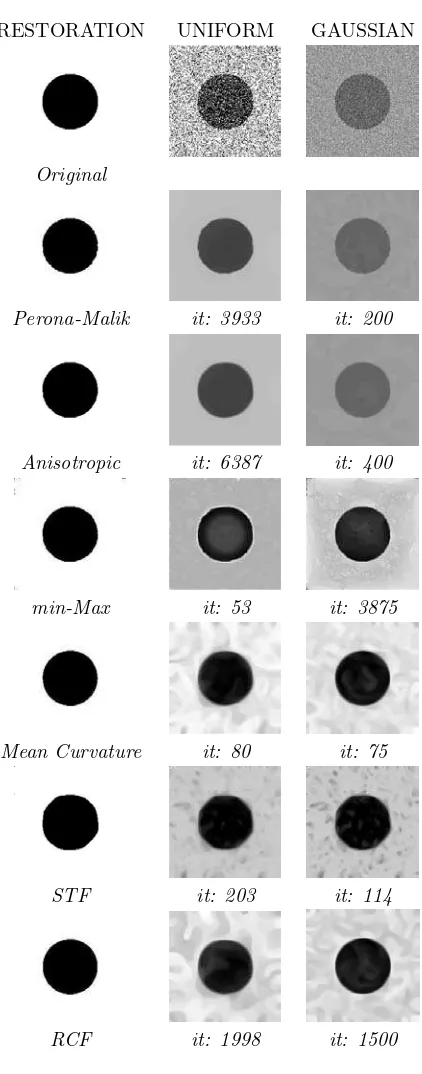
Figure 5.1 displays results for the M-shape and figure 5.2 for the circle. Best per-formances (second columns for uniform noise and third for gaussian one) correspond to the images achieving the best SNR. The number of iterations necessary to reach these images is displayed underneath. Shapes recovered (first columns), correspond to uniform noise, for the M-shape, and gaussian noise, for the circle.

The visual quality of the restored images (fig.5.1 and fig.5.2) is similar for all methods. Background artifacts in some images filtered with RCF are common to all geometric flows. Geometric flows are designed to smooth curves rather than images, therefore they are always prone to produce funny patterns in noisy backgrounds. This is not a main inconvenience if the aim of the filtering procedure is to restore a shape, which is the natural application of geometric flows. In fact, all reconstructed shapes have similar quality, matching the original templates. In the case of STF the circle hexagonal-like appearance could be improved by increasing the number of vertices of the final STF state.

We note that the number of iterations needed to achieve optimal restorations varies with noise.

Step 2: Asymptotic Behavior

Evolution of quality measurements in time (fig.5.3-5.5) reflects convergence to non trivial steady states as well as resemblance between original and evolved images. Final states after 3000 time units are overimpressed on the graphics of fig.5.5.

RESTORATION UNIFORM GAUSSIAN

Original

Perona-Malik it: 3425 it: 157

Anisotropic it: 3186 it: 164

min-Max it: 176 it: 4721

Mean Curvature it: 47 it: 21

STF it: 167 it: 74

RCF it: 825 it: 293

Figure 5.1: M-shape Best Reconstructions.

RESTORATION UNIFORM GAUSSIAN

Original

Perona-Malik it: 3933 it: 200

Anisotropic it: 6387 it: 400

min-Max it: 53 it: 3875

Mean Curvature it: 80 it: 75

STF it: 203 it: 114

RCF it: 1998 it: 1500

0 500 1000 1500 2000 2500 3000 −30 −25 −20 −15 −10 −5 0 5 10 15

20 SNR M−SHAPE GAUSSIAN 0.5

RCF MMF

MCF AD PMM

STF

0 500 1000 1500 2000 2500 3000 0

5 10 15 20

25 CTN M−SHAPE GAUSSIAN 0.5

MMF RCF AD MCF PMM STF

0 500 1000 1500 2000 2500 3000 0

5 10 15 20

25 CTN M−SHAPE 50% UNIFORM MMF RCF MCF PMM AD STF

(a) (b) (c)

Figure 5.3: M-Shape Quality Numbers Graphics

0 500 1000 1500 2000 2500 3000 −30 −20 −10 0 10 20

30 SNR CIRCLE 50% UNIFORM AD

MCF STF

MMF

PMM RCF

0 500 1000 1500 2000 2500 3000 0 2 4 6 8 10 12

14 CTN CIRCLE 50% UNIFORM RCF STF MMF MCF PMM AD

0 500 1000 1500 2000 2500 3000 0 5 10 15 20 25 30 35

40 CTN CIRCLE GAUSSIAN 0.5

RCF MMF MCF PMM AD STF

(a) (b) (c)

Figure 5.4: Circle Quality Numbers Graphics

PMM, MCF) present a maximum and then tend to zero at a rate related to the speed of convergence.

Diffusion processes (AD, PMM) fail to maintain quality numbers, especially for CTN values (fig.5.3, 5.4 (b), (c)). The decay is more significant in the measure noise increases and is more prominent in the case of gaussian noise. Geometric flows are more robust against the nature of noise and are more sensitive to the geometry of the underlying shape (see CTN graphics in fig.5.3 (b), (c) and fig.5.4). As expected, MCF is, by no means, the worst performer, especially when non-convex shapes are evolved (fig.5.3, fig.5.5 (a)). Among all techniques, RCF and MMF graphics are the only ones that match, for all cases, the model of a non-trivial steady state. Final images in fig.5.5 reflect quality numbers stability.

BecauseStep 2discards MCF and PMM,Step 3will only be applied to AD, MMF, STF and RCF.

Step 3: Evolution Stabilization

The stopping parameters areǫ= 10−3_{for critA and{ǫ= 10}−4_{T = 100}for critB. We} will keep the former stopping values for the remains of the paper. In order to produce an experiment as balanced as possible, we have tried the criteria on the gaussian noisy M-shape and the uniform noisy circle.

(a)

(b)

Figure 5.5: Asymptotic behavior in terms of SNR: (a) uniform noisy M-shape and (b) gaussian noisy circle

in the case of gaussian and uniform noise, respectively. Images stabilized using critA are shown in fig.5.7, 5.10 and those achieved with critB in fig.5.8 and fig.5.11.

appli-5000 10000 15000 20000 25000 0

0.5 1 1.5 2 2.5 3 3.5 4 4.5

x 10−4 AD SPEED

500 1000 1500 2000 2500 3000 3500 4000 4500 0

0.05 0.1 0.15 0.2 0.25

MMF SPEED

(a) (b)

0 500 1000 1500 2000 2500 3000 0

1 2 3 4 5 6 7

x 10−3 STF SPEED

500 1000 1500 2000 2500 0

0.5 1 1.5 2 2.5

x 10−3 RCF SPEED (g)

(c) (d)

Figure 5.6: Speed Graphics for gaussian noise on the M-shape

cability. If they asymptotically converge to zero, both criteria are valid, CritA is still applicable if plots just tend to zero, while CritB is satisfied for speeds asymptotically converging to a (positive) value. It follows that oscillating or irregular speeds difficult stopping the iterative process.

(a) AD (b) MMF

(c) STF (d) RCF Figure 5.7: Criterion A

(a) AD (b) MMF

(c) STF (d) RCF Figure 5.8: Criterion B

2000 4000 6000 8000 10000 12000 14000 0

5 10 15

x 10−4 AD SPEED

1000 2000 3000 4000 5000 6000 7000 −0.01

−0.005 0 0.005 0.01 0.015 0.02 0.025 0.03

MMF SPEED

(a) (b)

0 1000 2000 3000 4000 5000 6000 7000 8000 0

0.002 0.004 0.006 0.008 0.01

STF SPEED

500 1000 1500 2000 2500 3000 3500 4000 4500 5000 0

2 4 6 8 10 12

x 10−4 RCF SPEED (g)

(c) (d)

measure (fig.5.6 and fig.5.9 (d)) presents a smooth enough asymptotic behavior as to apply critB without strict restrictions. Besides, since RCF is a good noise remover, images in fig.5.8 and fig.5.11 (d) are close to the ones getting best quality numbers in fig.5.1 and fig.5.2.

For all methods, round-off errors in combination with the method behavior difficult success of critA. In the case of AD, rapid convergence to a constant image makes critA stop the evolution at too blurred images (fig.5.7(a)). For MMF, critA reveals to be efficient to stabilize images (fig.5.7, 5.10 (b)), although they may be far from final states because of evolution irregularity. Images obtained with STF present similar anomalies than those achieved with critB. The compromise between noise removal and shape preservation may not be achieved with a fixed ǫ. It follows that the M-shape image (fig.5.7 (c)) still presents background noise, while the circle of the clear image in fig.5.10 (c) starts differing from the theoretical final hexagon that, according to [79], should be the one of maximum size inside the circle. Finally, numeric errors induced by the embedding image may over-erode shapes smoothed with RCF (fig.5.7, 5.10 (d)).

For assessment of quality of the restored shapes in the case of highly noisy images, we will use critA for MMF, STF and critB for RCF.

(a) AD (b) MMF

(c) STF (d) RCF

Figure 5.10: Criterion A

(a) AD (b) MMF

(c) STF (d) RCF

Figure 5.11: Criterion B

Step 4: Robustness

In order to assess robustness, we have corrupted the M-shape with a gaussian noise of parametersµ= 0.5,σ= 1 (fig.5.12 (a)) and a 70% of uniform noise (fig.5.12 (e)). We have chosen a gaussian noise of positive mean in order to determine the dependence of each of the methods on the gray-level,α0, defining the curve of interest. We recall that this value is inherent to MMF formulation, as it switches between evolution by negative and positive curvature, while RCF only uses the parameter in its numeric implementation.

arti-ORIGINAL MMF STF RCF

Figure 5.12: Highly noisy M-shape, 1st row gaussian and 2nd uniform

ORIGINAL MMF STF RCF

Figure 5.13: Shapes for high noise, 1st row gaussian and 2nd uniform

facts than those that MMF yielded (fig.5.12(b), (f)). However, reconstructed shapes (fig.5.13(d), (h)) are more accurate and smoother for RCF filtered images. Shapes ob-tained with MMF (fig.5.12(b), (f)) still present irregularities and those obob-tained with STF may hardly resemble the original ones because of an insufficient noise removed. The higher irregularity in MMF reconstructions for gaussian noise, reflects its undesirable dependency on the gray-levelα0. In the case of RCF, dependency reduces, in the worst case, into an over erosion of the target shape.

We conclude that not only is our method the one achieving the best compromise between quality of restored image and evolution stabilization, but also the best suited for a non-user intervention application.

5.1.3

Experiment III. Application to Image Filtering and Shape

Recovery

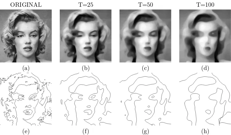
ORIGINAL T=25 T=50 T=100

(a) (b) (c) (d)

(e) (f) (g) (h)

Figure 5.14:Stop parameters impact on RCF filtering of Marilyn, gray-level images are in 1st row and descriptive level set in 2nd one

The following set of real images has been tested:

Faces and Real Objects

The portrait of Marilyn (fig.5.14 (a)) will serve to illustrate the role of T in RCF numeric scheme. We run RCF with ǫ = 10−3 _{and T = 25,50,100. Figure 5.14} displays the Marilyn’s gray-level images (first row) and the target level curve (second row). Images stabilized with the shortest time intervals (fig.5.14 (b), (c)) keep the most descriptive facial features (eyes, mouth and nose), while spurious details in the hair have been removed (see curves in fig. 5.14 (f), (g)). Besides, although the smoothest Marilyn image (fig.5.14 (d)) may seem rather eroded, the essential facial features are still identified in the target curve (fig.5.14 (h)).

We have chosen the buildings of fig.5.15 (a), (e) for our first comparison between RCF, MMF and STF. Because of their different geometric designs, they will illustrate capability of each of the methods to retain shape models in practical applications. The squared shaped arch of fig.5.15 (a) is perfectly kept by MMF (fig.5.15 (d)) and, though a bit rounder, by RCF (fig.5.15 (b)). Although we used the same parameters than in [79], rectangles have almost disappear in the STF image (fig.5.15 (c)). In the case of fig.5.15 (e), oval arch nicely appears in all filtered images fig.5.15 (f), (g) and (h). Although the ones in RCF image (fig.5.15 (e)) are sharper than in MMF smoothed building (fig.5.15 (g)) and smoother than in STF image (fig.5.15 (f).

ORIGINAL RCF STF MMF

(a) (b) (c) (d)

(e) (f) (g) (h)

Figure 5.15: Buildings filtering

RCF STF MMF

0 500 1000 1500 2000 2500 3000 3500 4000 4500 5000 0.01 0.02 0.03 0.04 0.05 0.06 0.07

0.08 FUNCTION g ON WHOLE IMAGE

200 400 600 800 1000 1200 1400 1600 1800 2000 −0.02 0 0.02 0.04 0.06 0.08 0.1 0.12

SPEED ON WHOLE IMAGE

200 400 600 800 1000 1200 1400 1600 1800 2000 2200 0 0.05 0.1 0.15 0.2 0.25

SPEED ON WHOLE IMAGE

(a) (b) (c)

0 500 1000 1500 2000 2500 3000 3500 4000 4500 5000 0 0.01 0.02 0.03 0.04 0.05

0.06 FUNCTION g ON SELECTED CURVE

200 400 600 800 1000 1200 1400 1600 1800 2000 0

5 10 15 x 10−3

SPEED ON SELECTD LEVEL SET

200 400 600 800 1000 1200 1400 1600 1800 2000 2200 0 0.02 0.04 0.06 0.08 0.1 0.12 0.14 0.16 0.18

SPEED ON SELECTED LEVEL SET

(d) (e) (f)

Figure 5.16: Speeds on whole image (1st row) and on selected curve (2nd row) for (a), (d) RCF, (b), (e), STF and (c), (f) MMF

selected curve are smoother in time, which motivates using the latter for evolution stabilization. We note that graphics reflect the error in RCF implementation (Section 2.5): peaks in fig.5.16(d) correspond to the error introduced by the collapsing of a small level curve.

preser-(a) (b)

(c) (d)

(e) (f)

(g) (h)

Figure 5.17: Filtering of plate:(a), (b) original, (c), (d), RCF (e), (f) MMF and (g), (h) STF

vation of geometric flows and RCF higher efficiency for shape restoration. Curves in the 2nd column correspond to image canny edges. We argue that the filtering should preserve image sharpness and regularity of the numbers and letters borders (fig.5.17 (b)), while superfluous details (small letters at the plate bottom and stamps) and noise that may mislead a latter segmentation process should be removed. First notice that all three geometric flows stabilize images (fig.5.17 (c), (e) and (f)) with contrast changes equal to the original. Edges (fig.5.17 (d)) of RCF final image yield plate numbers that, though a bit smoother, perfectly match the original ones. Mean-while, edges extracted from images stabilized with MMF and STF (fig.5.17 (f), (h)) are over-smoothed and the geometry (and even topology) of the resulting numbers is significantly different.

Application to Medical Images

(a) (b) (c) (d)

Figure 5.18:Cross Sections of IVUS sequences. Original IVUS images (a) and seg-menting curve (b), steady state attained with RCF (c) and the resulting segseg-menting curve(d).

(a) (b) (c)

Figure 5.19: Longitudinal cut of IVUS (a), shape segmenting blood and tissue in (b) the original cut and the smoothed shape with RCF (d).

the speed stabilization criterion over the level curve that best segments blood and tissue.

(a) (b) (c) (d)

Figure 5.20:Test Set 1. Noisy images: non convex shape (a), smoothed image (b), character ’S’ (c) and smoothed image (d).

(a) (b)

(c) (d) (e)

Figure 5.21: Test Set 2. Real images: human brain (a), horse (b), hand (c), horse head (d) and fingerprint (e).

5.2

Anisotropic Contour Closing

Restricted Diffusion

Anisotropic differential operators are widely used for image enhancement and restora-tion. However the capability of smoothly extending functions to the whole image domain has been hardly exploited.

As stated in chapter 1, functional extensions are governed by parabolic PDE’s, which equal that of heat diffusion processes except for the boundary conditions. We saw that the process has naturally associated a metric, given by the diffusion tensor, that locally describes the way heat extends or distributes. Thus an anisotropic heat diffusion is the analytic way of handling a dilation with non-constant elliptic structural elements. In the context of level sets completion the tensor should degenerate/cancel in the gradient direction, which might not guarantee existence of solutions of the associated PDE. In the present chapter, we perform a study of diffusion tensors from the point of view of differential geometry which provides us with a criterion to decide when such degenerate tensors still produce solvable PDE’s. We will define a new family of differential operators that locally restrict diffusion to the tangent spaces of image level sets. A particular instance of such operators results in an Anisotropic Contour Closing (ACC) that reduces the completion problem to the definition of a smooth vector field representing the level sets to be extended.

4.1

Restricted Anisotropic Operators

Any second order partial differential operator, namely L, defines, both, a diffusion process:

ut=Lu with u(x,0) =u0(x)

and a functional extension:

Lu= 0 with u|γ =f

for γ a curve in the image domain. In both cases, existence and uniqueness (in the weak sense) of smooth solutions is guaranteed if Lis strongly elliptic [23], [72], that is, when it defines a scalar product on some functional space. However, extensions focused on level sets continuation should restrict diffusion to a vector field representing

the level sets of the solution. Thus, the hypothesis of strong ellipticity is relaxed and we must tackle with operators that degenerate on some vector fields.

Let us give some geometric requirements over the non null space ofLthat ensure existence of solutions in the case of an operator given in divergence form. In this case, we have that:

Lu= div(J∇u)

forJ a symmetric (semi) positive defined tensor (quadratic form). Strong ellipticity means that all eigenvalues ofJ are strictly positive, meanwhile tensors having a null space (kernel) of positive dimension will produce degenerate operators. The fact that scalar products are given by symmetric (semi) positive defined tensors, motivates embedding elliptic operators into the framework of Riemmanian geometry to study the degenerate case. Details regarding results on differential geometry can be found in [67].

Let (Rn, g) be a Riemmanian manifold with the metric, g, given by a tensor J. Since the matrix J is symmetric, it diagonalizes [44] (considered as linear map) in an orthonormal basis that completely describes the metric. If Q is the coordinate change, then we have that, as bilinear form,J =QΛQt, for Λ the eigenvalue matrix. In this context,isotropicdiffusion corresponds to equal eigenvalues,anisotropicto distinct and strictly positive andrestricted 1 _{to the case of null eigenvalues. That} is, the restricted diffusion is given by a diffusion tensor, ˜J, defined by the following eigenvalue matrix: Λ =          

λ1 · · · 0 ..

. . .. ... 0 · · · λm

0 · · · 0 ..

. . .. ... 0 · · · 0 0 · · · 0

..

. . .. ... 0 · · · 0

0 · · · 0 ..

. . .. ... 0 · · · 0

         

Indeed we will only consider the homogeneous case λi = 1, for all i. Let us

deter-mine under what conditions a degenerated metric makes sense. Letξ1, . . . , ξk be the

eigenvectors of positive norm and denote byD=ξ1, . . . , ξkthe vector space

(distri-bution) they generate. If such vector space was the tangent space to a sub manifold of

Rn(integral variety ofD), then the metric ˜J would be the projection onto its tangent space. Consequently a diffusion process governed by ˜J would not take place in the whole spaceRnbut just on the integral manifolds, namelyM, of the distribution. We claim that this integrability condition and compactness are the only requirements for a unique solution to:

div( ˜J∇u) = 0 with u|γ =f (4.1)

which is as smooth as the boundary function f. We remit the reader to Section 4.3 for rigorous mathematical arguments concerning the above and the next statements. Let us devote the rest of the Section to intuitive reasonings on the precise meaning

1_{The word restricted applies to the the fact that diffusion restricts to the manifolds generated by}

of equation (4.1), those cases which always satisfy the integrability condition and applications to image processing.

Although (4.1) does not coincide with the heat equation for manifolds, the effect of the operator div( ˜J∇u) may be regarded as diffusing on each of the integral manifolds separately. For u|M =uM not only solves an elliptic second order equation in the

manifoldM, but also enjoys of the same properties as solutions to the heat equation in Rn:

1. Maximum Principle: the extreme values of the solutionuM are achieved on the

boundary M ∩∂Ω. In the particular case of a single generator, ξ, as M is a curve, the effect of restricting diffusion is that the final extension changes linearly along the level lines ofξ. Figure 4.1 is an example of functional extension in an image. The function to be extended is a color map defined on the ring of fig.4.1(a). The vector,ξ, guiding extension is the sinusoidal of fig.4.1(b) where the extension scope has been restricted to the area enclosed by the ring. The linear rate of change of the final extension (fig.4.1(d)) along theξintegral curves is better visualized in fig.4.2. The mesh representation of fig.4.2(a) is a cut of the mesh surface of u in the ξ direction, the corresponding plot for uM is in

fig.4.2(b). Because we have not achieved the steady state, the functionuM does

not linearly interpolate the values at the boundary as it happens in the plot of fig.4.2(d).

(a) (b) (c) (d)

Figure 4.1:General Extension: Function to extend (a), extension vector (b), inter-mediate step (c) and final extension (d)

2. Smoothness: the functionuM is smooth, providedf|M is also differentiable. Let

us show the reader that the hypothesis thatξcan be integrated (i.e. induces a foliation) on the domain is essential in order to guarantee convergence to smooth functions. The vector shown in fig.4.3(a) has a singular point at the center of the image since all its integral curves meet there. Although the extension process still exists, it converges to the sharp image of fig.4.3(b), which has a jump discontinuity at the center of the image as it shows the angular cut of the mesh of fig.4.3(c).

(a) (b)

(c) (d)

Figure 4.2:Rate of change along integral curves: intermediate step (a) with function plot (b) and final state (c) with function plot (d)

(a) (b) (c)

Figure 4.3: Singular Case: vector field (a), extension (b) and angular cut (c)

generated by the distribution can form a mesh or not. We note that for k ≥2 the integral curves of the vectorsξk will not, in general, tangle into a web. For instance,

ξ1=∂y = (0,1,0) andξ2=−y∂x+∂z= (−y,0,1) generate the curves of fig.4.4(b),

which as do not knit a mesh will never produce a surface. Meanwhile, the integral curves ofξ1=∂y andξ2=x∂x+∂zform mesh surfaces (fig.4.4(a)) which decompose

the space in layers (leaves of the foliation). An important remark for the foregoing discussion is that in the case of a single vector ξthe integrability condition is always satisfied.

(a) (b)

Figure 4.4:Frobenius Theorem: integrable (a) and non integrable (b) distributions

The instances of the process 4.1 relevant in image processing are the following:

1. Image Restoration

IfM is closed and transversal to the foliation and∇f ⊂ D⊥_{, then the leaves of} the foliation,M, describe the level sets of the extensionu, coinciding in the case of ann−1 dimensional distribution. This follows from the fact that if∇f⊥D, then we have that∂Ω∩M ⊂ {f ≡const} and, thus,u|M is constant. Besides

if dimD=n−1, as∇f =∇u, our restricted diffusion conforms to the Gestalt principle that requires that level sets continuation should be differentiable at boundary junctions. That is, the solutions suit to the idea of reliable image restoration.

In this case, the restricted diffusion should be regarded as a simultaneous inte-gration of all manifolds having as tangent spaceD. This drives (4.1) very close to the system of PDE’s used by [4] for image in-painting. The main advan-tage of our formulation is that it admits a simple implementation using a finite difference Euler scheme for a non-linear heat equation.

2. Image Enhancement and Filtering

The time-dependent parabolic equation associated to the restricted diffusion:

ut= divRn( ˜J∇u)

level sets. Because diffusion is performed along image level sets, image features are enhanced, in the sense that they are of uniform gray-level in the final image. Although this version of (4.1) resembles the diffusion of [9], there are some relevant differences. First of all, the degenerate differential operator:

ut= 1

1 +|∇u|2uξξ (4.2)

used in [9] can not be interpreted as a diffusion restricted to the integral curves of ξ. This follows because, given a functionu=u(x1, . . . , xn) onRn, its divergence

on a manifold embedded inRn is given by:

divM(J∇u) =

m

∇u, ξmM ·divM(ξm) +

m

ξm(∇u, ξmM) =

=

m

uξm·divM(ξm) +

m

uξmξm+

m

∇u, ξm(ξm)

for uξmξm the second derivative in the direction ξm. It follows that even in the case of div(ξm) = 0, the equation (4.2) can either be written in divergence

form nor interpreted as diffusing the function just on the integral curves of ξ. Meanwhile the development of (4.1):

divRn( ˜J∇u) =

m

∇u, ξmM·divRn(ξ_m) +

m

ξm(∇u, ξmM)

is a second order operator on the integral manifolds, which coincides with a heat kernel in the case of null divergence.

Besides lacking of a geometric interpretation, it is not guaranteed that steady states of (4.2) are non trivial. This fact forces adding the usual close-to-data constraint [62] or relying on a given number of iterations to ensure preservation of the image most relevant features. Its geometric nature makes our restricted diffusion evolution equation converge to a non trivial image that preserves the original image main features as curves of uniform gray level.

3. Contour Closing

If the manifoldM is included in one of the leaves of the foliation associated to Dand f|M =const, the restricted diffusion corresponds to curve continuation

and surface gap filling. This is the case we will focus on.

4.2

Anisotropic Contour Closing

(a) (b) (c)

(d) (e) (f)

Figure 4.5:Gap filling: clover (a), ridges of its mask extension (b), (c), image graph of uncomplete clover (d), intermediate step (e) and closing (f).

distributing heat only in the tangent direction, makes these curves evolve towards a closed contour of uniform gray level.

Therefore if we use this restricted anisotropic operator to extend a binary map of a unconnected curve (i.e. its characteristic function), the final state will be a binary map of a closed model of the uncomplete initial contour. This process is the Anisotropic Completion of Contours we suggest:

ut= div( ˜J∇u)

u|γ =u0 (4.3)

withu0the characteristic function of the opened contours,χγ, and the diffusion tensor

˜

J as described in the previous paragraph. Figure 4.5 illustrates the different stages in the process of gap filling for an incomplete clover (fig.4.8(a)). Ridges of the final characteristic function (fig.4.8(f)) correspond to the reconstructed complete contour (fig.4.8(c)).

From the above considerations, computation of an extension conforming to the image reduces to giving a smooth vector field representing its level curves.

4.2.1

Coherence Vector Fields

compute the vector fieldξ. Notice that since orientations do not play any role in the diffusion process, the eigenvectors ofStserve to design diffusion tensors [72].

The Structure Tensor is usually employed to determine the direction of maximum contrast change of an imageuin a robust way [72]. Given an integration scale,ρ, it is defined as the mean of the projection matrices,P(∇uσ), onto a regularized image

gradient:

Stρ=Gρ∗P(∇uσ) =Gρ∗(∇uσ⊗ ∇uσ) =Gρ∗ ∇uσ∇uTσ

where Gρ denotes a centered gaussian of variance ρ and ∇uσ = Gσ ∗ ∇u. The

eigenvector of minimum eigenvalue,ξ, (coherence direction) corresponds to the level sets unit tangent direction.

Since by convolving with a gaussian we obtain solutions to the heat equation, we have that the Structure Tensor benefits from the regularizing and extension properties of diffusion processes. The matrixStρis the solution to the heat equation with initial

condition the projection matrix onto the image gradient vector space. This implies that the coherence direction, ξ, is a infinitely differentiable field [24] that regularizes and extends the level curves unit tangent space. This property is the key point for the definition of the different Coherence Vector Fields. We will note byγ0the contour to be closed and byt0 its tangent space.

(a) (b)

Figure 4.6: LVF extension (a) of tangent vector at a gap (b)

1. Linear Vector Fields (LVF).

They are the coherence direction of the Structure Tensor compute over the characteristic functionχγ0. By the above properties, ξis a smooth vector field

defined (i.e. non zero) in a neighborhood ofγ0that correctly matchest0at gap boundaries and coincides with it at other points. Figure 4.6 shows the gradient ofχγ0 (fig.4.6 (b)) used to compute the vectorξof fig.4.6 (a). Sinceξscope may

(a) (b) (c)

Figure 4.7: DVF extension: distance map (a), tangent spaces (b), DVF (c)

(a) (b) (c) (d)

Figure 4.8:Corners Extension: LVF (a), LVF closure (b), DVF (c) and closure (d)

Note that LVF is nothing but the coherence direction of the convolutionGσ∗χγ0,

which level sets might be regarded as a propagation of the original curve. The fact that geometric flows are the natural way of propagating and deforming shapes leads to:

2. Distance Vector Fields (DVF).

Letu be a function representing the evolution of γ0 under a monotonous ge-ometric flow, γt = β−→n, with β > 0. That is, the level sets, u ≡ c, coincide

with the evolution ofγ0 at timet=c. Notice that at a suitable time/scale, ρ, (gap dependent) the level curves of this distance map have only two connected components that model a closure ofγ0(fig.4.7(a)). It follows that the coherence direction,ξ, models a closure ofγ0 (fig.4.7(c)) that smoothly interpolatest0 at gaps and is not singular at corners (fig.4.8(c)). The shapes obtained are smooth models (fig.4.8(d)) of the original shape based on the principle of minimum dis-tance for joining boundary points. Although, this is a desirable property, in the particular case of a distance between contours smaller than the gap size, LCV is preferable, as DVF closed models do not conform to the shape yielded by our visual system. For instance, DVF reconstruction of the broken lines of fig. 4.9(a) are not two straight lines, as expected, but the curves of fig.4.9 (b). We remit the reader to the experiments in chapter 5.2 for illustrative examples on the choice of the coherence vector field in practical applications

(a) (b) (c) (d)

Figure 4.9: DVF pathology: lines (a), DVF (b), final extension (c), DVF closure (d)

(a) (b) (c)

(d) (e) (f)

(g) (h) (i)

Figure 4.10: Dynamic Closing of Contours

the current image evolution every k iterations. The initial DVF (fig.4.10(a)) closes the smallest gaps and reduces the length of the gaps in the ridges (fig.4.10(c)) of the evolved image (fig.4.10(b)). DVF over the distance map of image ridges yields a vector field (fig.4.10(d)) that closes all gaps with the exception of the largest one (fig.4.10(e), (f)), which is the most delicate since we must interpolate a piece of high curvature. The DVF that finally closed this gap is the vector field of (fig.4.10(g)). Ridges of the final extension (fig.4.10(h)) are the reconstructed shape of fig.4.10(i) and represent a smooth and accurate completion of the contour regardless of the magnitude of the curvature.

4.3

Mathematical Issues

This section deals with the mathematical arguments that yield existence of solutions to the restricted diffusion. In mathematical formal terms, the problem is stated as follows. Let Ω be a compact subset of Rn with a smooth boundary, ∂Ω, and let f =f(x1, . . . , xn) be a smooth function defined on∂Ω. We seek for solutions to the

following extension problem:

div( ˜J∇u) = 0 with u|∂Ω=f (4.4)

for ˜J the projection matrix onto a distribution D = ξ1, . . . , ξk transversal to ∂Ω

almost everywhere:

˜ J =



 

ξ1 .. . ξk



 

Idk 0

0 0

(ξ1, . . . , ξk)

Because the diffusion tensor cancels on some curves, standard arguments on elliptic PDE do not apply. One way of proving existence and uniqueness to (4.4) could be through viscosity solutions [23], [20]. We, instead, will approach the problem from a differential geometry point of view and show that (4.4) yields a heat equation on the integral varieties of the distribution D (if it is involutive), which coincides with the laplacian operator [21] for manifolds provided that the divergence of the fields ξi is

zero. Existence of solutions on a generic leave of the folliation suffices to guarantee existence and uniqueness of functionsu=u(x1, . . . , un) solving the restricted diffusion

problem (4.4) inRn.

4.3.1

Solutions to the Problem on Manifolds

In order to show that (4.4) is solvable on a generic leave,M, we will first compute its expression in local coordinates and, then, construct a solution.

Relation between Restricted Diffusion and the Heat Equation for Mani-folds

vector field by divN(·), Lie derivatives byL and the Lie bracket by [·,·]. We recall

that if (x1, . . . , xN) are local coordinates, then the partial derivatives∂xi are a basis of the tangent spacesTpNand its dual,dxi, are a basis of the cotangent (linear forms)

T∗

pN.

It follows that, in local coordinates, a vector fieldξequalsξk_∂

xk, the derivative, ξ(f), of any smooth functionf :N →Ris given by:

ξ(f) =ξk∂xkf

and the metric by a (symmetric) matrix (gij)ij. Furthermore, if g = det(gij) is its

determinant, then the volume form equalsω =g1/2_{dx1. . . dx}

N. The divergence of a

vector fieldξ can be defined as the Lie derivative ofωalongξ:

Lξω= divN(ξ)ω

The quantity measures the change of a unit of volume along the integral curves of ξ (fig. ....). The fact [67] that:

ξ(ω(∂x1, . . . , ∂x1)) = (Lξω)(∂x1, . . . , ∂x1)−

i

ω(∂x1, . . . ,[ξ, ∂xi], . . . , ∂x1)

yields that the expression of divN(ξ) in local coordinates is:

divN(ξ) =g−1/2ξ(g1/2) +

i

∂xi(ξ

i_{) (4.5)}

Given a smooth function,f, it has an associated form,df, defined as:

df(ξ) =ξ(f) =ξk∂xk(f)

The gradient, ∇f, of such function it is defined [21] asj−1(df), for:

j:TpN →Tp∗N

the isomorphism given by the metricj(ξ)(η) :=ξ, ηN. It follows that:

∇f, ξN =j(j−1(df))(ξ) =ξ(f) (4.6)

The above formulae (4.5), (4.6) are the only expressions we need to compute (4.4) in the local coordinates of a generic leaveM. IfM is a manifold embedded inRn, then given a coordinate chart:

φ: U ⊂Rk −→ M ⊂Rn

s= (s1, . . . , sk) → (φ1(s), . . . , φn(s)) =x

The vector fields∂si are given by∂si(φ) = (φ 1

si, . . . , φ

n si) =φ

1

si∂x1+· · ·+φ

n