A hybrid algorithm combining metaheuristic with Monte Carlo simulation for solving the Stochastic Flow Shop problem
22
0
0
Texto completo
(2) The study of the SFSP is within the current popularity of introducing randomness into combinatorial problems. It allows to describing new problems in new realistic scenarios where some information cannot be obtained previously. It is important to remark the FSP as a relevant topic for current research, so a large set of efficient optimization, heuristic and metaheuristic methods have been developed. As it has happened with other combinatorial problems, a large number of different approaches and methodologies have been developed to deal with it. These. approaches. range. from. pure. optimization. methods. (such. as. linear. programming) for dealing with small-sized problems to use of heuristic and metaheuristics to provide near-optimal solutions for medium and large-sized problems. Usually, the main criterion to minimize is the makespan, but other criteria different to total time employed to process the list of jobs should also be considered in order to provide the decision-maker a large set of near-optimal and efficiently obtained options where he/she could choose according to specific necessities. The main difference between the FSP and the SFSP is that in the former job processing times are known beforehand, while in the latter the actual processing time of each job has a stochastic nature, i.e. the statistical distribution is known beforehand, but its exact value is revealed only when the job is to be launched. So, while in the deterministic problem the performance measure is usually the makespan, in the non deterministic version this measure is not representative. This is due to the fact that we do not know the execution times of the jobs involved, so it has no sense to talk in terms of concrete values but in terms of probability. So, we must consider the expected makespan to have a valid way of measuring the performance. As a result, our final target is to minimize the expected makespan of the obtained sequences. Besides, there are a large set of methods developed for the FSP. This is not the case of the SFSP. These methods need to be efficient to provide near optimal solutions to small and medium instances of the problem in a reasonable time. The rest of this work is structured as follows: in section 2 the SFSP is presented with a detailed formulation and section 3 provides a literature review in order to expose an overview of the state of the art. In section 4 the main ideas of our approach are explained, and section 5 discusses the advantages offered by our methodology over the existing to date.. Section 6 shows numerical experiments. that illustrate our methodology, with a discussion of its results in the Section 7..
(3) Section 8 describes future work to perform on related topics. Finally, section 9 summarizes the main contributions of this paper.. 2. Basic notation and assumptions The SFSP is a well-known scheduling problem that can be formally. described as. follows: a set J of n independent jobs have to be processed on a set M of m independent machines. Each job every machine. j ∈ J requires a stochastic processing time pij n. i∈ M . This stochastic processing time is defined by a certain. distribution (e.g. normal, exponential, triangular, etc.). The classical goal is to find a sequence for processing the jobs so a given criterion is optimized. The most common used criterion is the minimization of the maximum completion time or makespan, denoted by Cmax. The described problem is usually denoted as Fm|prmu|C max, which means that it is a flow-shop permutation problem with m machines with the aim to minimize the makespan. In addition to this definitions, it is assumed that: •. all the jobs are processed in all the machines in the same order.. •. there is unlimited storage between the machines, and non-preemption.. •. machines are always available.. •. each machine can process only one job a time.. •. a job cannot be processed more than once for machine.. •. job. processing. times. are. independent. and. exponentially. distributed. variables. At this point, it is interesting to notice that our approach does not require to assume any concrete distribution for the stochastic variable whereas it is in most previous stochastic flow shop approaches.. 3. State of the art and related work The FSP is a NP-complete problem (Rinooy kan 1976) which consists, as mentioned, in running a set of J jobs in a set of M machines with the goal of minimizing total execution time or makespan. We focus on the stochastic version, where jobprocessing times follow probability distributions.. The first publication about flow. shop scheduling with random processing times appears in Markino (1965), where a problem with two machines and two jobs is presented..
(4) Many works have focused on the importance of considering uncertainty in real world problems, specifically in the case of scheduling-related problems. Thus, Al-Fawzan et al. (2005) analyzes the Resource Constrained Project Scheduling Problem (RCPSP) focusing on makespan reduction and robustness. Jensen (2001) also introduces. the. concepts. of. neighborhood-based. robustness. and. tardiness. minimization. Ke (2005) proposes a mathematical model for achieving a formal specification of the Project Scheduling Problem. Allaoui (2006) studied makespan minimization and robustness related to the SFSP, suggesting how to measure the robustness. Proactive and reactive scheduling are also characterized in his work. An example of reactive scheduling can be found on Honkonp (1997), where performance is evaluated using several methodologies. On the other hand, robustness in proactive scheduling is analyzed in Ghezail et al. (2010), who propose a graphical representation of the solution in order to evaluate obtained schedules. As the concept of minimum makespan from FSP is not representative for the stochastic problem, Dodin (2006) proposes an optimally index to study the efficiency of the SFSP solutions. The boundaries of the expected makespan are also analyzed mathematically. A theoretical analysis of performance evaluation based on markovian models is performed in Gougand et al. (2005), where a method to compute expected time for a sequence using performance evaluation is proposed. A study of the impact of introducing different types of buffering among jobs is also provided in this work. On the other hand, Integer and linear programming has been employed together with probability distributions to represent the problem in Janak 2007. Many heuristics and metaheuristics have been proposed in order to solve the PFSP due to the impossibility of finding exact solutions efficiently. For example, Johnson (1954) suggested a simple heuristic to solve the two machines problem, while Campbell et al. (1970) built a heuristic for PFSP with more than two machines. NEH is considered the best performing heuristic, it was introduced by Nawaz et al. (1983).. Later, Tailard (1990) reduced NEH complexity by introducing a data. structure to avoid the calculation of the makespan. Moreover, Ruiz (2005) proposed an Iterated Greedy (IG) algorithm for the PFSP built on a two-step methodology. Some successful works have been published about dealing with indeterminacy in other combinatorial problems as the Vehicle Routing Problem (VRP), with Stochastic Demands (VRPSD). The VRPSD is a variation of the VRP, where the demands to serve are unknown and follow certain probability distributions..
(5) In some recent works, Juan et al. (2009a, 2009b, 2010a) describes the application of simulation technologies to solve Vehicle Routing Problems. Thus, in Juan et al. (2011), the stochastic problem is transformed into a deterministic instance using the concept of safety-stocks as a confidence margin over the variance of the demands. This subsequent deterministic problem is solved employing proven efficient heuristics. Then, simulation is applied in order to evaluate the probability of failure of the obtained sequences. Simulation has been applied in the SS-GNEH (Juan et al. 2010b) to solve the FSP in , where the NEH algorithm is modified to have some random behavior building a GRASP-like methodology. In the stochastic variant, simulation based approaches usually rely on performance evaluation as in Gougard (2003). Dodin (2006) performs simulations to prove its empirical analysis of the boundaries of the makespan. Moreover, Honkonp (1997) relies on the use of simulation for reactive scheduling while Ghezail et al. (2010) graphical representation that has been mentioned previously.. 4. Proposed methodology The main idea behind the methodology is that the initial stochastic problem (SFSP) will be transformed into a deterministic version (FSP), where well-known heuristics exist. Because well-tested meta-heuristics exists for the FSP, such as SS-GNEH, we will apply it in order to get some efficient solutions for this deterministic problem. The transformation is achieved by assigning the expected value associated to the probability distribution that described the stochastic job processing time, to the deterministic. As any feasible solution for the deterministic instance is also a potential solution for the SFSP, we can extrapolate it to the stochastic scenario. Then, we estimate the expected makespan for the stochastic problem by using the direct Monte Carlo method. So the obtained solution will be simulate in the probabilistic scenario. The simulation will be run as many times as we need to get an estimation reliable enough. The specific steps describing the proposed methodology are the following: 1. Consider a SFSP instance defined by a set J of jobs and a set of M machines with stochastic processing times for each job in each machine..
(6) 2. Consider for each job with processing time p ij the expected value for the corresponding probability distribution: p*ij = E[pij]. 3. Let be FSP* the resulting problem defined by the deterministic demands p*ij . 4. Generate some efficient random solutions for the FSP* by applying a proven heuristic such as SS-GNEH. 5. For each feasible solution generated, run some simulations in order to obtain an estimation of the expected makespan (the more simulations we perform, the more exact estimation is obtained). 6. Store the best stochastic and deterministic solutions 7. Calculate a more exact expected makespan estimation for both solutions 8. Test that the stochastic solution is the best, change for the deterministic otherwise 9. Output the solution The graphical representation of this process is as follows:.
(7) 4.1 Algorithm Pseudo-code The pseudo-code 1 shows the main procedure of our test execution, which drives the methodology..
(8) procedure Main for each instance from test2run begin solution = StochasticSSGNEH.solve(instance) end lowerBound = getBestDeterministicSolution() SimulateStochastic(GetBestDeterministicSolution(), 100000) //Compute Upper-bound getBestStochasticSolution() ShowSolutions. First inputs are entered in the program and each test is run for solving each problem instance using proposed methodology. After that, the lower and upper bounds are calculated in order to test the efficiency of the obtained solution.. At. last, solution is provided to the output.. StochasticSSNGEH.solve(instance) //For each feasible solution generated during the SSGNEH calculus solution = SSGNEH.solve(instance) // Deterministic algorithm solution.stochasticCost = getStochasticCost(solution, 1000) storeBestDeterministicSolution(solution) //Current best deterministic solution storeBestStochasticSolution(solution) //Current best stochastic solution improveEstimation() return solution. Pseudo-code 2 offers the main procedure of our methodology, where the stochastic cost is estimated for each feasible solution obtained by the SS-GNEH when solving the deterministic problem. We run the necessary simulations in order to obtain a first and efficient approximation of this cost.. Once the cost is estimated it is. compared to the cost of the best stored solution, if it is better, we choose this latter solution as candidate. This steps will be performed for all the solutions provided by the deterministic problem associated. Pseudo-code 3 provides the details of the Monte Carlo simulation of the stochastic scenario.. Here, we will iterate over all jobs and all machines to construct the. distribution associated to each permutation. library for stochastic simulation.. To do that we will rely on the SSJ. Next, we generate random values from the. distribution for constructing a probabilistic scenario. Once we have obtained values for all pairs of job and machines we calculate the cost of the given solution and, after running as many simulations as we the number we passed in parameters we return the mean from all values..
(9) getStochasticCost(solution, simulations) for i from 1 to simulations do begin for each job in solution.jobs begin for each machine in solution.machines begin dist = ExponentialDistributionFromMean(solution.cost(job, machine)) ExponentialGen gen = new ExponentialGen(dist) stochasticTimes.cost(job, machine) = dist.nextDouble end end makespan = calcost(stochasticTimes) //calcost is the same cost calculation algorithm adapted to double values makespanSum = makespanSum + makespan; end return makespanSum/simulations. Pseudo-code 4 exemplifies the way of improving the solution quality. First we run stochastic simulations both for the best deterministic solution and the best stochastic solution stored.. We do that as many times as we need to get a. estimation reliable enough.. Finally, we compare the expected makespans to test. that the proposed best solution stays between the bounds. If it is no so, we correct it. improveEstimation() if (SimulateStochastic(GetBestDeterministicSolution(), 100000) < SimulateStochastic(GetBestStochasticcSolution()) then storeBestStochasticSolution(GetBestDeterministicSolution()) end. 5. Advantages and contribution of our approach Despite the idea of solving a stochastic problem by solving a related deterministic problem is not completely new (see the state of art section), it has not been developed for solving the SFSP. In fact, most of the works to date have focused in the theoretical aspects of the stochastic scheduling. By contrast, the proposed method provides a practical approach to the solution, with some potential benefits. The potential benefits of our approach are: •. While previous approaches rely on theoretical chance-constrained models, our approach suggests a more practical perspective. This allows us to deal with more realistic scenarios..
(10) •. By using Monte Carlo simulation in our methodology, it allows to build models based in different random variables while previous approaches use to assume a particular behavior. More exactly, any probability distribution for describing the job processing times could be implemented with no restriction.. Thus, as far as we know, the presented methodology offers some unique advantages over the existing to date for solving the SFSP. In fact, some of these potential benefits are: •. The methodology is valid for any statistical distribution with a known mean, both theoretical -e.g. Normal, Log-normal, Weibull, Gamma, etc.- and experimental.. •. The methodology reduces the complexity of the SFSP -where no efficient methods are known yet- to the FSP, where mature and extensively tested heuristics have been developed. This increases the credibility of the provided final solution.. •. Because it is based on simulation, the methodology can be extended to consider a different distribution for each job processing time, possible dependencies among jobs, etc.. •. The methodology can be applied to SFSP instances of virtually any size, so complexity attached to size can be managed by efficient SFSP metaheuristics and Monte Carlo simulation.. In summary, the benefits provided by our methodology can be summarized in two points: simplicity and flexibility.. It is simple because is parameter-free and does. not need fine tunning and flexible because it can be adapted to other probabilistic scenarios of virtually any size or admit more variables.. 6. A numerical experiment Described methodology has been implemented as a Java application.. Java. language was selected because of being an object oriented language that facilitates the rapid development of a prototype.. A standard personal computer Intel(c) 7i. CPU a t 2.6 GHz and 3 GB RAM was used to perform all test, which where run directly from the Eclipse IDE. There is a lack of specific benchmarks for the SFSP, this could be due to the mentioned fact that most works about the problem have been mainly theoretical. So we have decided to use a benchmark created for the deterministic FSP..
(11) In order to test our heuristic with that deterministic test we assume that, in each test instance, the processing time for each job is considered as the mean of the probabilistic distribution associated to that job in the stochastic case. After that, we generate random values based on the resulting distribution function. We have tested 90 instances from Taillard tests (1993) with different seeds and we have generate probabilistic values based on triangular distributions. For each instance, we have considerate the solution given by the NEH heuristic, the best solution obtained with the SS-GNEH heuristic for the deterministic case. and the. best solution obtained for the deterministic scenario. In addition, to generate probabilistic values, we use a triangular distribution defined with the parameter. =1/ E x , being E(x) the expected value. This distribution. and the probabilistic generation of random values are implemented using the SSJ library. for. stochastic. simulation. that. can. be. found. in. http://www.iro.umontreal.ca/~simardr/ssj/. Before discussing the results of the methodology, we will focus in one instance of the tests to illustrate our methodology.. Given tai001_20_5 instance from the. Taillard tests with the following processing times: Job. Machine 1. Machine 2. Machine 3. Machine 4. Machine 5. 1. 54. 79. 16. 66. 58. 2. 83. 3. 89. 58. 56. 3. 15. 11. 49. 31. 20. 4. 71. 99. 15. 68. 85. 5. 77. 56. 89. 78. 53. 6. 36. 70. 45. 91. 35. 7. 53. 99. 60. 13. 53. 8. 38. 60. 23. 59. 41. 9. 27. 5. 57. 49. 69. 10. 87. 56. 64. 85. 13. 11. 76. 3. 7. 85. 86. 12. 91. 61. 1. 9. 72. 13. 14. 73. 63. 39. 8. 14. 29. 75. 41. 41. 49. 15. 12. 47. 63. 56. 47. 16. 77. 14. 27. 40. 87. 17. 32. 21. 26. 54. 58. 18. 87. 86. 75. 77. 18. 19. 68. 5. 77. 51. 68.
(12) 20. 94. 77. 40. 31. 28. First, we solve this deterministic instance using the SS-GNEH algorithm, in the first iteration we obtain the permutation of jobs: 3,15,6,19,14,9,17,18,5,7,8,16,4,11,13,1,2,10,20,12. With the associated cost 1279. After that, we convert it to a stochastic case by considering these processing times as the mean of associated probabilistic distribution functions.. So, we obtain the. following stochastic instance:. Job. Machine 1. Machine 2. Machine 3. Machine 4. Machine 5. 1. 54. 79. 16. 66. 58. 2. 83. 3. 89. 58. 56. 3. 15. 11. 49. 31. 20. 4. 71. 99. 15. 68. 85. 5. 77. 56. 89. 78. 53. 6. 36. 70. 45. 91. 35. 7. 53. 99. 60. 13. 53. 8. 38. 60. 23. 59. 41. 9. 27. 5. 57. 49. 69. 10. 87. 56. 64. 85. 13. 11. 76. 3. 7. 85. 86. 12. 91. 61. 1. 9. 72. 13. 14. 73. 63. 39. 8. 14. 29. 75. 41. 41. 49. 15. 12. 47. 63. 56. 47. 16. 77. 14. 27. 40. 87. 17. 32. 21. 26. 54. 58. 18. 87. 86. 75. 77. 18. 19. 68. 5. 77. 51. 68. 20. 94. 77. 40. 31. 28. Next, we apply Monte Carlo Simulation in order to obtain the expected makespan of this job ordination. To achieve that, we generate random processing times based on the constructed probability distribution (triangular distribution as it has been stated) obtaining the following values:.
(13) Job. Machine 1. Machine 2. Machine 3. Machine 4. Machine 5. 1. 53.952316644188 9.5543248590763 4.0598198283469 21.437067621716 8.3490954601264 64 63 91 718 42. 2. 10.851787267698 91.460056769749 35.837638859000 146.08657218939 18.461884218872 429 44 35 328 605. 3. 3.0081763388665 74.078892936058 2.5904531998378 387.37039921251 16.076462561126 252 18 104 807 057. 4. 46.192910414844 0.8149869032398 40.636353639872 40.695167559803 122.12764384230 733 894 36 167. 5. 94.562946920758 1.1772624863448 55.260163551225 2.6845595432183 22.531359012907 98 413 42 68 842. 6. 29.033858900786 3.3387275950179 55.707495886166 53.680221591405 9.6515409760194 257 99 69 92 4. 7. 5.6135407117047 3.2676925492616 68.659793009468 76.289193105274 123.77580750894 08 085 32 36 643. 8. 133.19271923095 15.179903613315 11.996223935475 19.538318354179 13.294782802073 39 757 877 047 815. 9. 26.188254555213 47.513074471646 160.84541592595 85.441358016844 44.749508551404 46 4 713 38 45. 10. 68.972098947363 53.439719287521 69.875857451882 3.4468622162152 98.976245941413 96 63 14 41 96. 11. 20.530964355405 23.430624201722 1.5795915612903 315.28867284935 82.868280270012 11 324 546 02 28. 12. 29.071211748509 31.391331640945 17.297742306435 309.15581777055 40.639925084991 57 022 15 96 61. 13. 9.2887025539540 173.82359494129 9.9766572665323 277.60993359429 9.4069543231754 97 724 3 38 41. 14. 197.19307601188 0.2046532114187 18.564442931524 79.494589648374 2.2999123787184 643 86 002 77 05. 15. 28.898575955178 11.916628000834 98.291276703511 8.4164417342996 3.2180761986050 63 773 19 26 38. 16. 7.9001750537592 66.124718700783 17.127595253307 202.17297185734 18.960013984275 44 2 533 25 502. 17. 21.827587127837 0.0400051972441 101.56883829078 62.580178844182 14.068610008992 15 8818 609 704 977. 18. 143.44762013909 139.36158099887 34.154855080851 94.316425867253 5.4491531895991 87 038 895 93 54. 19. 41.837844341648 0.4146954457302 26.593006064417 21.204220278958 30.918277881247 83 1266 743 33 05. 20. 25.631890535301 20.568620521375 0.4261491289961 11.570901789733 110.69251455482 313 948 6536 627 81. Subsequently, we calculate the total cost of a problem with the obtained solution and generated processing times values to obtain the cost of 2519.1844962101795. If we repeat this calculation 1000 times, we obtain a first approximation to the expected makespan: 1796.8382775738291. We store both deterministic and stochastic values (as we are in the first iteration it is the best solution until now) and run next iteration to obtain another feasible solution from SS-GNEH: 9,17,8,3,6,19,15,1,2,13,4,14,11,5,18,16,10,7,20,12.
(14) We follow the same procedure to compare the new obtained costs (a deterministic cost of 1286 and a stochastic cost of 1774.8112823703784) with the previous obtained values and we store the best solution both cases. By performing this procedure 100000 times we are able to obtain an estimated best deterministic solution, and a estimated best stochastic solution. Now, a more exact value of the expected makespan of both solutions can be calculated by running previous simulation more number of times. If we find that when the cost estimation is improved, the best stochastic solution cost is greater than the the best deterministic solution stochastic cost (which could be expected because of the nature of the random-based calculation), we correct it by taking the best deterministic solution as the the best stochastic one too. At the end of the calculations, we would obtain the output with the best solutions found and its calculated and estimated costs:.
(15) *************************************************** * RESULTS FROM SIMSCHEDULING PROJECT * *************************************************** -------------------------------------------NEH Solution -------------------------------------------Sol ID : 1 Sol deterministic costs: 1286 Sol time: 0h 0m 0s (0.002992901 sec.) List of jobs: 3 17 9 8 15 14 11 16 13 19 6 4 5 18 1 2 10 7 20 12. -------------------------------------------Our best deterministic solution (provided by the SS-GNEH) -------------------------------------------Sol ID : 8 Sol deterministic costs: 1278 Sol stochastic costs: 1770.877998309444 Sol time: 0h 0m 0s (0.172264997 sec.) List of jobs: 9 3 17 6 15 14 11 13 5 4 19 8 18 7 16.
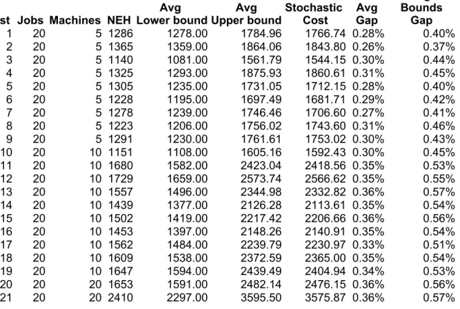
(16) 7. Results In this section, we will study the result obtained in the test simulation. Because we have run 15 executions of each instance with different seeds, we provide average values for each instance from all the executions. In addition, we have presented them in a table that shows the following values: •. The number of the Taillard's test instance. •. The jobs in the problem. •. The machines in the problem. •. The deterministic cost associated to the NEH solution. •. The deterministic cost associated to the SS-GNEH solution as the average lower bound. •. The average stochastic cost of the SS-GNEH solution as the upper bound.. •. The average stochastic cost of the best stochastic solution. •. The average gap of the stochastic solution with the lower bound.. •. The average gap between the upper and the lower-bounds is provided in order to study the variance between these bounds.. Table 1 shows the results for the first 30 instances. These instances consider cases with 20 jobs.. Test Jobs Machines 1 20 5 2 20 5 3 20 5 4 20 5 5 20 5 6 20 5 7 20 5 8 20 5 9 20 5 10 20 10 11 20 10 12 20 10 13 20 10 14 20 10 15 20 10 16 20 10 17 20 10 18 20 10 19 20 10 20 20 20 21 20 20. Avg Avg Stochastic NEH Lower bound Upper bound Cost 1286 1278.00 1784.96 1766.74 1365 1359.00 1864.06 1843.80 1140 1081.00 1561.79 1544.15 1325 1293.00 1875.93 1860.61 1305 1235.00 1731.05 1712.15 1228 1195.00 1697.49 1681.71 1278 1239.00 1746.46 1706.60 1223 1206.00 1756.02 1743.60 1291 1230.00 1761.61 1753.02 1151 1108.00 1605.16 1592.43 1680 1582.00 2423.04 2418.56 1729 1659.00 2573.74 2566.62 1557 1496.00 2344.98 2332.82 1439 1377.00 2126.28 2113.61 1502 1419.00 2217.42 2206.66 1453 1397.00 2148.26 2140.91 1562 1484.00 2239.79 2230.97 1609 1538.00 2372.59 2365.00 1647 1594.00 2439.49 2404.94 1653 1591.00 2482.14 2476.15 2410 2297.00 3595.50 3575.87. Avg Gap 0.28% 0.26% 0.30% 0.31% 0.28% 0.29% 0.27% 0.31% 0.30% 0.30% 0.35% 0.35% 0.36% 0.35% 0.36% 0.35% 0.33% 0.35% 0.34% 0.36% 0.36%. Avg Bounds Gap 0.40% 0.37% 0.44% 0.45% 0.40% 0.42% 0.41% 0.46% 0.43% 0.45% 0.53% 0.55% 0.57% 0.54% 0.56% 0.54% 0.51% 0.54% 0.53% 0.56% 0.57%.
(17) 22 23 24 25 26 27 28 29 30. 20 20 20 20 20 20 20 20 20. 20 20 20 20 20 20 20 20 5. 2150 2411 2262 2397 2349 2362 2249 2306 2277. 2099.00 2329.00 2223.00 2291.00 2226.00 2273.00 2202.00 2237.00 2179.00. 3298.44 3639.60 3460.68 3602.36 3479.58 3557.57 3454.92 3504.33 3387.19. 3281.61 3617.91 3442.83 3582.25 3457.01 3533.57 3445.28 3494.48 3382.62. 0.36% 0.36% 0.35% 0.36% 0.36% 0.36% 0.36% 0.36% 0.36%. 0.57% 0.56% 0.56% 0.57% 0.56% 0.57% 0.57% 0.57% 0.55%. Table 2 shows the results for the instances 31 to 60. These are larger instances with 50 jobs. We can intuitively observe that the gap takes similar values as in the 30 first instances. Nevertheless, we can notice that the gaps are reduced for the first test with fewer machines.. Test Jobs Machines 31 50 5 32 50 5 33 50 5 34 50 5 35 50 5 36 50 5 37 50 5 38 50 5 39 50 5 40 50 10 41 50 10 42 50 10 43 50 10 44 50 10 45 50 10 46 50 10 47 50 10 48 50 10 49 50 10 50 50 10 51 50 20 52 50 20 53 50 20 54 50 20 55 50 20 56 50 20 57 50 20 58 50 20 59 50 20 60 50 20. Avg Avg Stochastic NEH Lower bound Upper bound Cost 2733 2724.00 3522.70 3459.28 2843 2834.00 3731.96 3694.60 2625 2621.00 3427.64 3388.20 2782 2751.00 3638.33 3592.25 2868 2863.00 3703.07 3618.92 2835 2829.00 3742.09 3693.47 2736 2725.00 3597.94 3560.16 2690 2683.00 3537.44 3487.79 2571 2552.00 3377.34 3341.84 2786 2782.00 3622.38 3564.36 3136 3025.00 4506.76 4482.79 3021 2909.00 4334.14 4317.21 2952 2864.00 4279.23 4274.24 3183 3063.00 4537.90 4512.48 3128 2997.00 4478.06 4457.64 3158 3006.00 4487.17 4467.46 3277 3124.00 4605.84 4566.63 3123 3042.00 4467.61 4437.44 3002 2902.00 4324.26 4299.90 3257 3090.00 4604.51 4582.18 4013 3893.00 6182.12 6159.07 3921 3725.00 5914.06 5905.13 3890 3684.00 5846.34 5829.94 3926 3759.00 5952.62 5932.24 3822 3647.00 5820.71 5803.73 3914 3723.00 5848.38 5832.61 3952 3736.00 5909.25 5897.86 3916 3732.00 5898.40 5888.76 3952 3780.00 5980.83 5973.08 4016 3786.00 5996.64 5985.04. Avg Gap 0.21% 0.23% 0.23% 0.23% 0.21% 0.23% 0.23% 0.23% 0.24% 0.22% 0.33% 0.33% 0.33% 0.32% 0.33% 0.33% 0.32% 0.31% 0.33% 0.33% 0.37% 0.37% 0.37% 0.37% 0.37% 0.36% 0.37% 0.37% 0.37% 0.37%. Avg Bounds Gap 0.29% 0.32% 0.31% 0.32% 0.29% 0.32% 0.32% 0.32% 0.32% 0.30% 0.49% 0.49% 0.49% 0.48% 0.49% 0.49% 0.47% 0.47% 0.49% 0.49% 0.59% 0.59% 0.59% 0.58% 0.60% 0.57% 0.58% 0.58% 0.58% 0.58%.
(18) At last, table 3 shows the results for the instances 61 to 90. These are the largest instances with 100 jobs. We can see that, following the tendency suggested by the former table, the gaps keep reducing for low number of machines. In contrast, the gap increases for larger number of machines.. Test Jobs Machines 61 100 5 62 100 5 63 100 5 64 100 5 65 100 5 66 100 5 67 100 5 68 100 5 69 100 5 70 100 5 71 100 10 72 100 10 73 100 10 74 100 10 75 100 10 76 100 10 77 100 10 78 100 10 79 100 10 80 100 10 81 100 20 82 100 20 83 100 20 84 100 20 85 100 20 86 100 20 87 100 20 88 100 20 89 100 20 90 100 20. Avg Avg Stochastic NEH Lower bound Upper bound Cost 5516 5493.00 6809.01 6717.21 5284 5268.00 6545.44 6496.53 5195 5175.00 6443.60 6382.25 5023 5014.00 6236.39 6171.95 5261 5250.00 6522.29 6458.81 5139 5135.00 6360.45 6305.33 5259 5246.00 6442.84 6415.35 5105 5094.00 6335.86 6281.29 5489 5448.00 6756.58 6710.72 5332 5322.00 6622.95 6576.24 5825 5771.00 7983.92 7937.18 5400 5349.00 7420.98 7386.03 5755 5679.00 7764.55 7715.57 5924 5791.00 8080.19 8045.43 5612 5478.00 7593.95 7560.71 5355 5308.00 7318.32 7271.01 5677 5596.00 7649.66 7605.66 5705 5630.00 7775.75 7752.52 5975 5880.00 8056.98 8005.56 5903 5848.00 7991.28 7936.59 6538 6281.00 9527.45 9517.08 6446 6263.00 9460.01 9432.26 6552 6343.00 9565.22 9548.23 6547 6333.00 9523.62 9485.02 6614 6389.00 9669.60 9643.86 6645 6481.00 9747.78 9722.86 6573 6337.00 9639.99 9623.97 6747 6493.00 9848.87 9835.94 6601 6355.00 9641.51 9623.66 6670 6503.00 9716.32 9694.36. Avg Gap 0.18% 0.19% 0.19% 0.19% 0.19% 0.19% 0.18% 0.19% 0.19% 0.19% 0.27% 0.28% 0.26% 0.28% 0.28% 0.27% 0.26% 0.27% 0.27% 0.26% 0.34% 0.34% 0.34% 0.33% 0.34% 0.33% 0.34% 0.34% 0.34% 0.33%. Avg Bounds Gap 0.24% 0.24% 0.25% 0.24% 0.24% 0.24% 0.23% 0.24% 0.24% 0.24% 0.38% 0.39% 0.37% 0.40% 0.39% 0.38% 0.37% 0.38% 0.37% 0.37% 0.52% 0.51% 0.51% 0.50% 0.51% 0.50% 0.52% 0.52% 0.52% 0.49%. In order to discuss these results, some visual support could be helpful. Thus, graph 1 provides the graphical representation of the calculated gaps, a quick view shows that best results are obtained in instances 31-40 and 61-70 where the number of machines is lower. We can observe that the gap seems to be greater the more machines there are.. In contrast, it appears to generate quite similar values for. same number of machines, no matter how many jobs are involved.. So, it could. suggest that this approach has potential power with problems with a large numbers of jobs..
(19) 0.70%. 0.60%. 0.50%. 0.40%. 0.30%. 0.20%. 0.10%. 0.00% 2 1. 4 3. 6 5. 8 7. 9. 10 12 14 16 18 20 22 24 26 28 30 32 34 36 38 40 42 44 46 48 50 52 54 56 58 60 62 64 66 68 70 72 74 76 78 80 82 84 86 88 90 11 13 15 17 19 21 23 25 27 29 31 33 35 37 39 41 43 45 47 49 51 53 55 57 59 61 63 65 67 69 71 73 75 77 79 81 83 85 87 89. On the other hand, graph 2, provides a graphical representation of the result comparatively with upper and lower-bounds.. Here, we can clearly see that the. obtained solution is always closer to the upper-bound than to the lower-bound. So, it seems to be some margin in order to improve the quality of the methodology. 12000.00. 10000.00. 8000.00. Avg Lower bound Avg Upper bound Stochastic Cost. 6000.00. 4000.00. 2000.00. 0.00 2 4 6 8 10 12 14 16 18 20 22 24 26 28 30 32 34 36 38 40 42 44 46 48 50 52 54 56 58 60 62 64 66 68 70 72 74 76 78 80 82 84 86 88 90 1 3 5 7 9 11 13 15 17 19 21 23 25 27 29 31 33 35 37 39 41 43 45 47 49 51 53 55 57 59 61 63 65 67 69 71 73 75 77 79 81 83 85 87 89.
(20) 8. Conclusions and future work In this paper we have presented a probabilistic approach for solving the Stochastic Flow Shop Problem. This methodology combines Monte Carlo simulation with well tested methodologies for the Flow Shop Problem. The one of the basic ideas of our methodology is to decompose the SFSP into several FSP in order to obtain an estimation of the expected makespan for an efficient solution to the deterministic case by using simulation. This approach does not require any previous assumption and is feasible for any probabilistic function. As a future work, some ideas are proposed. First, qualitative studies can be performed in order to compare robustness or different optimality measures. Next, the development of an approach which uses parallelization to perform the different scenarios of the simulation in different threads. We think this could improve performance and help to achieve more exact estimations of the expected makespan. The use of C/C++ versions of the code could reduce the computation times. Also, the study of the use of a security margin when transforming the stochastic problem into deterministic instances could improve the robustness and efficiency of the obtained solutions.. 9. References Allaoui, H.; Lamouri, S.; Lebbar, M., 2006, A robustness framework for a stochastic hybrid flow shop to minimize the makespan, In Proceedings of the International Conference on Service Systems and Service Management, 1097-1102. Al-Fawzan, M.; Haouari, M , 2005, A bi-objective model for robust resourceconstrained project scheduling, International Journal of Production Economics. Campbell, H.G., Dudek, R.A., and M.L. Smith, 1970. A heuristic algorithm for the n job, m machine sequencing problem. Management Science 16, B630- B637 . Dodin, B., 2006, Determining the optimal sequences and the distributional properties of their completion times in stochastic flow shops, Computers & Operations Research 23(9), 829-843. Ghezail, F.; Pierreval, H.; Hajri-Gabouj, S. , 2010, Analysis of robustness in proactive scheduling: a graphical approach, Computers & Industrial Engineering 58, 193-198. Gourgand, M.; Grangeon, N.; Norre, S. , 2003, A contribution to the stochastic flow shop scheduling problem , European Journal of Operational Research 151, 415433 . Gourgand, M.; Grangeon, N.; Norre, S. , 2005, Markovian analysis for performance evaluation and scheduling in m machine stochastic flow-shop with buffers of any capacity, European Journal of Operational Research 161, 126-147..
(21) Honkomp, S.; Mockus, L.; Reklaitis, G. , 1887, Robust scheduling with processing time uncertainty, Computers & Chemical Engineering 21, 1055-1060. Janak, S.; Lin, X.; Floudas, C. , 2007, A new robust optimization approach for scheduling under uncertainty II. Uncertainty with known probability distribution, A new robust optimization approach for scheduling under uncertainty II. Uncertainty with known probability distribution. Jensen, M. T., 2001, Improving robustness and flexibility of tardiness and total flow-time job shops using robustness measures, Applied Soft Computing 1, 3552. Johnson, S.M., 1954. Optimal two- and three-stage production schedules with setup times included. Naval Research Logistics Quarterly 1, 61-68 Juan, A., Faulin, J., Ruiz, R., Barrios, B., Caballe, S., 2009a. The SR-GCWS hybrid algorithm for solving the capacitated vehicle routing problem. Applied Soft Computing 10, 215-224. Juan, A., Faulin, J., Ruiz, R., Barrios, B., Gilibert, M., Vilajosana, X., 2009b. Using oriented random search to provide a set of alternative solutions to the capacitated vehicle routing problem. In: Chinneck, J.; Kristjansson, B; Saltzman, M. (Eds) “Operations Research and Cyber-Infrastructure” OR/CS Interfaces Series 47, 331- 346. Springer, New York, USA. Juan, A., Faulin, J., Jorba, J., Riera, D., Masip; D., Barrios, B., 2010a. On the Use of Monte Carlo Simulation, Cache and Splitting Techniques to Improve the Clarke and Wright Savings Heuristics. Journal of the Operational Research Society, doi:10.1057/jors.2010.29. Juan, A.; Ruiz, R.; Mateo, M.; Lourenço, H. , 2010b, A simulation-based approach for solving the flow-shop problem, A simulation-based approach for solving the flow-shop problem. Juan, A.; Faulin, J.; Marull, J.; Jorba, J.; Marques, J. , Under Revision, Using Parallel & Distributed Computing for Solving Real-time Vehicle Routing Problems with Stochastic Demands, Annals of Operations Research. Juan, A.; Faulin, J.; Grasman, S.; Riera, D.; Marull, J.; Mendez, C. , In press, Using Safety Stocks and Simulation to Solve the Vehicle Routing Problem with Stochastic Demands, Transportation Research Part C, DOI 10.1016/j.trc.2010.09.007 . Ke, H.; Liu, B. , 2005, Project scheduling problem with stochastic activity duration times, Applied Mathematics and Computation 168, 342-353. Nawaz, M., Enscore, E.E., and I. Ham, I., 1983. A heuristic algorithm for the mmachine, n-job flowshop sequencing problem. OMEGA 11, 91-95. Rinnooy Kan, A.H.G., 1976. Machine Scheduling Complexity and Computations. Springer.. Problems:. Classification,. Rubén Ruiz, Concepción Maroto, 2005, A comprehensive review and evaluation of permutation flowshop heuristics, European Journal of Operational Research 165 (2005) 479–494..
(22) Taillard, 1990, Some efficient heuristic methods for the flow shop sequencing problem, European Journal of Operational Research 47 (1990) 65-74. Taillard, 1993, Benchmarks for Basic Scheduling Problems, European Journal of Operational Research 64 (1993) 278-285..
(23)
Figure

Documento similar