ROC performance evaluation of RADSPM technique

ROC performance evaluation of RADSPM technique

JAVIER GIACOMANTONE - ARMANDODEGIUSTI

Instituto de Investigaci´on en Inform´atica LIDI (III-LIDI) Facultad de Inform´atica - Universidad Nacional de La Plata

{jog,degiusti}@lidi.info.unlp.edu.ar

Abstract. The purpose of Functional Magnetic Resonance Imaging (fMRI) is to map areas of increased neuronal activity of the human brain. fMRI has been applied to inves-tigate a variety of neuronal processes from activities in the primary sensory and motor cortices to cognitive functions such as perception or learning. Robust anisotropic diffu-sion of statistical parametric maps (RADSPM) is a new technique to improve functional Magnetic Resonance Imaging. RADSPM attempts to improve voxel classification based on robust anisotropic diffusion (RAD) to include the spatial relationship between active voxels. This paper compares two fMRI postprocessing techniques used to identify areas of increased neuronal activity, a widely used method, correlation analysis, and RADSPM. In recent years, the use of ROC analysis has been extended from its original use in com-munication systems to machine learning, pattern classification and fMRI. We proposed to use ROC curves and the area under the curve (AUC) not only as a final performance evaluation and visualizing technique but as a gauging parameter procedure in RADSPM. We give a brief review of the main methods and conclude presenting experimental results and suggesting further research alternatives.

1

Introduction

A Receiver Operating Characteristic (ROC) analysis is a technique for evaluating and visualizing the performance of different classifiers. ROC analysis of functional Magnetic Resonance Imaging (fMRI) was introduced by Constable [1] in 1995. The purpose of Functional Magnetic Resonance Imaging (fMRI) is to map areas of increased neuronal activity of the human brain. The hemoglobin in the blood is a natural contrast agent, because it has different magnetic properties depending on its state of oxygenation [2]. These differences affect the voxel intensity in the magnetic resonance image. In a typical fMRI experiment, baseline images are scanned periodically while the subject is at rest (or in other baseline condition) and activation images are acquired when the subject is performing a specific task or receiving a stimulus. A classical method for identifying activated brain regions from noisy fMRI 4-D image is the correlation analysis [3]. A correlation coefficient measures the degree of matching between the time series of a particular voxel and the expected activation of the experiment design. For each correlation coefficient, a t-statistics is computed and spatially disposed, forming a Statistical Parametric Map (SPM). The classification of voxels as active or non-active is performed by thresholding the SPM at a particular significance level, without taking into account any spatial relationship between voxels.

RADSPM [4] is a technique based on Robust Anisotropic Diffusion (RAD) and classic correlation coefficient analysis that includes the spatial relationship and improves the detection of active voxels. We use ROC curves to show that the proposed technique is superior to the conventional correlation method and introduce the use of ROC analysis as a gauging method for adjusting the diffusion pa-rameter in RADSPM.

This paper is divided in two parts, sections 2 to 5 cover the fundamental ideas behind RADSPM and ROC analysis. Sections 6 and 7 show experimental results and propose future research work, involving extensive tests on fMRI images and parallel fMRI processing, based on the present results.

2

fMRI Correlation Analysis

Correlation analysis is a simple method widely used to detect active voxels in fMRI images [5]. Each voxel s has an associated time series Xs = {x1, x2, ...xN}, where N is the number of volumes of

the 4-D functional image. Y =_{y1, y2, ..., yN}is the reference time series, expected to represent the

oxygenation changes in the blood due to the experiment stimulation. The reference time series can be a simple square waveform representing the stimulation protocol, a delayed square waveform, or the convolution of a square waveform with the Hemodynamic Response Function (HRF) of the brain [6]. The sample correlation coefficient

ρs=

P

(xi−x)(yi−y)

pP

(xi −x)2

P

(yi−y)2

(1)

describes the matching between the observation and the expectation.

In order to classify the voxelsas active or non-active, we transform the correlation coefficientρsinto

the random variableτsthat follows Student´s t-distribution withN−2degrees of freedom:

τs =

ρs

√ N ₋2 p

1₋ρ2

s

(2)

The image obtained by spatially disposingτs, for every voxel s, is called statistical parametric map

3

Robust Anisotropic Diffusion

Perona and Malik [7] defined the anisotropic diffusion as

∂I(x, y, t)

∂t = div [g(k∇I(x, y, t)k)∇I(x, y, t)], (3)

using the original image I(x, y,0) : R2

→ R+ _{as the initial condition, wheret is an artificial time}

parameter and g is an “edge-stopping” function. The right choice of g can greatly affect the ex-tent to which discontinuities are preserved. Perona and Malik suggested two possible edge-stopping functions in their paper [7]. Black et al. [8] used the robust estimation theory to choose a better edge-stopping function, called Tukey’s biweight:

g(x) = ( h

1₋ x2

5σ2 i2

, x2

5 ≤σ 2

0, otherwise (4)

The functiongabove is the dilated and scaled version of the original Tukey’s function, whereg(0) = 1 and the local maxima of its “influence function”ψ(x) =xg(x)is situated atx=σ. The diffusion that uses the Tukey’s function is called robust anisotropic diffusion (RAD) and this is the edge-stopping function adopted in this paper.

Perona and Malik [7] discretized spatio-temporally their anisotropic diffusion equation (3) as:

I(s, t+ 1) =I(s, t) + λ |ηs|

X

p∈ηs

g(_|∇Is,p(t)|)∇Is,p(t), (5)

whereI(s, t)is a discretely sampled image,sdenotes the pixel position in a discrete 2-D or 3-D grid, t_≥0now denotes discrete time steps, the constantλdetermines the rate of diffusion (usually,λ = 1), and ηs represents the set of spatial neighbors of pixel s. For 2-D images, usually four neighbors

are considered: north, south, west and east, except at the image boundaries. For 3-D images, six voxels are usually considered: the above-mentioned four plus “up” and “down” voxels. The gradient magnitude of a voxel in a particular direction at iterationtis approximated by:

∇Is,p(t) = I(p, t)−I(s, t), p∈ηs. (6)

Black et al. [8] suggested to use the “robust scale” defined by:

σe= 1.4826 MAD(∇~I) = 1.4826 medianI

h

k∇~I_{k −}medianI(k∇~Ik)

i

, (7)

where MAD is the Median Absolute Deviation.

4

Anisotropic Diffusion of fMRI

averaging. It computes an initial set of clearly activated voxels. This set is then used to construct a complex “similarity measure” to calculate the averaging coefficients.

A new and different technique, directly related to the Robust Anisotropic Diffusion RAD, have been proposed to overcame the former drawbacks. It has been named Robust Anisotropic Diffusion of Statistical Parametric Maps (RADSPM) [11, 4].

RADSPM is simple and has yielded clear SPMs when applied to both simulated and real fMRI data. This technique increases substantially the statistical significance of activated regions, what makes it possible to decide with more confidence if a certain brain region is activated or not.

LetI′

be an fMRI data. First of all, the mean value is removed fromI′

, yielding the mean-removed fMRII:

I =I′

−I′ ₍₈₎

This pre-processing is very important, because structural and functional regions of the brain do not necessarily match. No structural information should be diffused, but only the activation information. Note that the activation information is not affected at all by the mean-correction.

Let us denote the fMRI data at iterationt _≥ 0of the diffusion process asI(s, n, t), whereI(s, n,0) is the initial mean-corrected fMRI at spatial voxel positions and volumen. RADSPM is described below:

1. Lett_←0.

2. Calculate the SPM(τ)T, using equations (1) and (2). Let us denote the value of the SPM(τ) at voxelsand iterationtasT(s, t).

3. Compute the diffusion coefficients. The diffusion coefficient between a voxels and its neigh-boring voxelpat instanttis:

g(_|∇Ts,p(t)|), where∇Ts,p(t) = T(p, t)−T(s, t). (9)

4. Use these coefficients to perform the diffusion inI(s, n, t), yielding the diffused fMRI I(s, n, t+ 1)at iterationt+ 1:

I(s, n, t+ 1)_←I(s, n, t) + λ |ηs|

X

p∈ηs

g(_|∇Ts,p(t)|)∇Is,p(t), (10)

where_∇Is,p(n, t) =I(p, n, t)−I(s, n, t).

5. Lett _← t+ 1and repeat steps 2 to 5 some predefined number of times or until the average of diffused values (second term of equation (10)) is below some predefined threshold.

5

ROC analysis

The result of postprocessing Magnetic Resonance images either with RADSPM or correlation analy-sis is another image named SPM(τ). Each voxel value represents the degree to which that particular voxel is a member of a class. A binary classifier is obtained by applying a threshold to the corre-sponding parametric map. In fact, for each different value of the threshold, a new binary classifier is defined. We refer to N as the number of negative or non-activated voxels and P as the number of positive or activated ones.

Given a binary classifier and the class membership of each voxel, that is, the ideal classification (gold standard), or the true class obtained from an artificial image (phantom), there are four possible results of the classification process:

True Positive (TP): positive voxels detected as positive.

True Negative (TN): negative voxels detected as negative.

False Positive (FP): negative voxels detected as positive.

False Negative (FN): positive voxels detected as negative.

The sum of TP, TN, FP and FN is the total number of voxels in the image. Usually this quantities can be represented as a contingency table or confusion matrix as indicated in table 1.

True Class

P N

Predicted Class P N

TP FP

FN TN

Table 1: Confusion matrix for binary classifiers

The principal diagonal of the confusion matrix represents the correct classification. A perfect classi-fication would only contain values different from zero in the main diagonal.

A number of common performance metrics can be derived from the the definitions of TP, TN, FP and FN [13]. The True Positive Fraction (TPF) and the False Positive Fraction are defined as:

T P F = T P

T P +F N (11)

F P F = F P

F P +T N (12)

Receiver Operating Characteristics (ROC) analysis has long been used in signal detection theory, medical diagnostic systems and functional neuroimaging analysis [1, 14, 15, 16]. ROC curves are graphs in which the TPF is plotted on the Y axis and the FPF is plotted on the X axis when a parameter of our detection method varies. Each binary classifier is defined by one point in the ROC space. The terminology used in ROC analysis includes terms like the sensitivity, or recall, or the TPF, and the specificity defined by equation (13).

specif icity= T N

A common definition of a ROC curve is as a graph of the sensitivity versus one minus specificity. A perfect classifier will have sensitivity and specificity equal to one, and a random one produces a ROC point on the line y=x. As a particular parameter of our classification model varies, we obtain a different binary classifier each one corresponding to a new point in the ROC space. The main impor-tant metrics derived from the ROC curve are the area under the curve (AUC) and the distance from the optimal operation point (OOP), where the latter is defined as the point of the curve more distant from the principal diagonal. In this work we proposed to use ROC analysis to compare statistical parameters maps obtained by correlation analysis and RADSPM for different activation thresholds.

6

Experimental Results

In order to test and develop classification models in fMRI we use an artificial image or a real image and the corresponding gold standard. In the first case we know the expected result, the exact location of activated and non-activated voxels, but it is difficult to simulate the noise distribution of noisy and complicated fMRI signal. Using real fMRI images requirers multidisciplinary efforts to determine the gold standard. The results presented in this section are based on the first approach, results of RADSPM on real fMRI images are reported in [11, 4]. We generated a simple artificial 4-D fMRI, with10_×10_×3voxels per volume and 84 volumes. Voxels values were 16000 corrupted by zero-mean Gaussian noise with standard deviationσ = 4000. Active voxels had their values increased by 1000 and 1500 for artificial images (A.I), that we also call phantom images I and II respectively. The fMRI had alternating blocks of 6 non-active and 6 active volumes, beginning with non-active volumes. Activated volumes had a6_×6_×3activated region in the center of the volume, with two non-activated regions of2_×2_×3voxels each.

Figure 1 depicts RADSPM’s and correlation’s ROC curves. Each point of a ROC curve is obtained by solving equations (11) and (12) for a specific threshold value.

(a) Phantom-I (b) Phantom-II

Figure 1: ROC curves

Table 2 presents performance metrics of the two ROC curves: (1) The area under RADSPM’s curve is larger than that of correlation’s; (2) The distance doop from the principal diagonal to the optimal

shows larger TPF, lower FPF and lower observed statistical significance levelpoopthan the correlation

method for both phantom I and phantom II.

Method Area dpo ppo T P Fpo F P Fpo

Correlation-SPM 0.7863 0.3063 0.3 0.7619 0.3287 Phantom-I

RADSP Mσ=1.8,t=10 0.9645 0.5687 0.0001 0.9524 0.1481

Correlation-SPM 0.8798 0.4373 0.2 0.8452 0.2269 Phantom-II

RADSP Mσ=2,t=10 0.9958 0.6594 0.00001 0.9881 0.0556

Table 2: Performance metrics

Figure 2 presents ROC curves for three different values of σ. The ROC curves can be seen as a gauging method to select the adequate diffusion parameter.

(a) Phantom-I (b) Phantom-II

Figure 2: (a)S1 = σe,S2 = 1.5σe,S3 = 1.86σeand (b)S1 =σe,S2 = 1.5σe,S3 = 1.73σe

Method T Ppo T Npo F Ppo F Npo

Correlation - SPM 64 145 71 20

Phantom-I

RADSPM(σ = 1_.8_{, t}= 10_{) 80 184 32 4}

Correlation - SPM 71 167 49 13

Phantom-II

RADSPM(σ= 2_{, t}= 10_{) 83 204 12 1}

Table 3: TP, TN, FP, FN

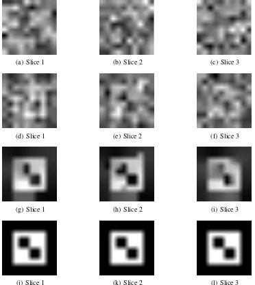
Figure 3 depicts one activated volume of the phantom II, the SPM(τ) generated by the correlation method, the SPM(τ) generated by RADSPM and the gold standard of the artificial image. Clearly, RADSPM has produced an SPM(τ) with better quality than the correlation map.

(a) Slice 1 (b) Slice 2 (c) Slice 3

(d) Slice 1 (e) Slice 2 (f) Slice 3

(g) Slice 1 (h) Slice 2 (i) Slice 3

(j) Slice 1 (k) Slice 2 (l) Slice 3

7 Conclusions and Future Work

In this paper we have presented ROC performance evaluation of a new technique named RADSPM and classical correlation analysis of fMRI time series. Experimental results using ROC curves have shown promising results for RADSPM parametric maps of artificial images. We have successfully used ROC analysis to adjust the diffusion parameter from an initial value ofσ. Further research in-volves improving the probabilistic model used to create the artificial images considering the noise distribution and the signal to noise ratio in order to approximate the complex and noisy fMRI signal structure. Extensive tests on real fMRI and artificial data must be done in order to extend our results to different real experiment paradigms. Magnetic Resonance scanners place huge demands on comput-ing and visualization capacity. Real time functional processcomput-ing involves multidisciplinary efforts [17]. At the expense of an increase in computational complexity RADSPM includes contextual information that improves the performance of the classification model, the processing time is the weak point for practical use of RADSPM in real time. In order to reduce the postprocessing time further research involves parallel fMRI processing [18] for image reconstruction, visualization and fundamentally for post-processing techniques.

8

Acknowledgments

The authors would like to thank Dr. Tatiana Tarutina for helpful discussions and comments that helped to improve the paper.

9

References

[1] R. T. Constable and Skudlarski P. An ROC approach for evaluating functional brain MR image analysis. Magnetic Resonance in Medicine, 34(1):57–64, 1995.

[2] S. Ogawa, A. R. Kay T.M. Lee, and D. W. Tank. Brain magnetic resonance imaging with contrast dependent on blood oxygenation. In Proc. Natl. Acad. Sci. USA, volume 87, pages 9868–9872, 1990.

[3] Peter A. Bandettini, A. Jesmanoswicz, Eric C. Wong, and James S.Hyde. Processing strategies for time-course data sets in functional mri of the human brain.Magnetic Resonance in Medicine, 30:161–173, 1993.

[4] Hae Yong Kim, Javier Giacomantone, and Zang Hee Cho. Robust Anisotropic Diffusion to Produce Enhanced Statistical Parametric Map. Computer Vision and Image Understanding, 99:435–452, 2005.

[5] J. Baudewig, P. Dechent, K. D. Merboldt, and J. Frahm. Thresholding in Correlation Analyses of Magnetic Resonance Functional Neuroimaging. Magnetic Resonance Imaging, 21:1121–1130, 2003.

[6] Gossl C., Auer D. P., and Fahrmeir L. Hemodynamic response function in bold fmri. NeuroIm-age, 14:140–148, 2001.

[7] P. Perona and J. Malik. Scale space and edge detection using anisotropic diffusion. IEEE.

[8] M. J. Black, G. Sapiro, D. H. Marimont, and D. Hegger. Robust anisotropic diffusion. IEEE

Transaction on Image Processing, 7(3):421–432, 1998.

[9] Hong Shan Neoh and Guillermo Shapiro. Using anisotropic diffusion of probability maps for activity detection in block-design functional mri. In Proceedings of the IEEE International

Conference on Image Processing, volume 1, pages 621–624, 2000.

[10] A. F. Sol´e, S. C. Ngan, G. Sapiro, X. P. Hu, and A. L´opez. Anisotropic 2-d and 3-d averaging of fmri signals. IEEE Transaction on Medical Imaging, 20(2):86–93, 2001.

[11] Hae Yong Kim, Javier Oscar Giacomantone, and Zang Hee Cho. Mapa Anisotr´opico Estad´ıstico de Im´agenes de Resonancia Magn´etica Funcional. In Proceedings, Buenos Aires, Argentina, 2004. Memorias del X Congreso Argentino de Ciencias de la Computacion.

[12] Voci F., Eiho S., Sugimoto N., and Sekiguchi H. Estimating the gradient threshold in the perona-malik equation. IEEE Signal Processing Mag., pages 39–46, 2004.

[13] Vuk M. and Curk T. Roc curve, lift chart and calibration plot. Advances in Methodology and Statistics, 3(1):89–108, 2006.

[14] Rajesh Nandy, Larissa Stanberry, and Dietmar Cordes. ROC methods with real fMRI data. In

Human Brain Mapping, 2003.

[15] J. A Sorenson and X. Wang. ROC Method for Evaluation of fMRI techniques. Magnetic

Reso-nance in Medicine, 36:737–744, 1996.

[16] Skudlarski Powel, Constable Todd R., and Gore John C. ROC Analisis of Statistical Methods Used in Funcional MRI: Individual subjects. Neuroimage, 9:311–329, 1999.

[17] Nigel Goddard, Greg Hood, Jonathan Cohen, William Eddy, Christopher Genovese, Douglas Noll, and Leigh Nystrom. Online analysis of functional mri datasets on parallel platforms. J.

Supercomput., 11(3):295–318, 1997.