Event-driven field estimation for wireless sensor networks

(1)

Sensor Networks

Daniel de O. Cunha1,2_{, Otto Carlos M. B. Duarte}1_{, and Guy Pujolle}2 ?

1_{Grupo de Teleinform´}_{atica e Automa¸c˜}_ao

Universidade Federal do Rio de Janeiro - UFRJ Rio de Janeiro, Brazil

2_{Laboratoire d’Informatique de Paris 6 (LIP6)}

Universit´e Pierre et Marie Curie - Paris VI Paris, France

Summary. This paper introduces and analyzes a field estimation scheme for wireless sensor networks. Our scheme imitates the response of living beings to the surrounding events. The sensors define their pe-riphery of attention based on their own readings. Readings differing from the expected behavior are considered events of interest and trigger the data transmission to the sink. The presented scheme is evaluated with real-site-collected data and the tradeoff between the amount of data sent to the sink and the reconstruction error is analyzed. Results show that significant reduction in the data transmission and, as a con-sequence, in the energy consumption of the network is achievable while keeping low the average reconstruction error.

1 Introduction

Recent advances in MEMS technology and wireless communications made pos-sible to embed sensing, processing, and communication capabilities in low-cost sensor nodes. As a consequence, the use of hundreds or thousands of nodes organized in a network [1] becomes an alternative to conventional sensing tech-niques. The resulting sensor network has the advantage of being closer to the sensed process, being able to acquire more detailed data.

Field estimation is an important application of wireless sensor networks. This type of application deploys sensor nodes in a specific region to remotely sense space-temporally variable processes, such as temperature or UV exposure. It is a continuous data-delivery application [2] and the simplest approach of such a system is based on deploying the sensors in the area of interest and requiring all the nodes to transmit data to the sink at a prespecified rate. The quality of the estimation depends of the spatial and temporal frequencies of sampling.

?

(2)

90 Daniel de O. Cunha , Otto Carlos M. B. Duarte , and Guy Pujolle

These frequencies must be high enough to avoid the aliasing problem [3]. Nev-ertheless, higher frequencies generate a larger amount of data to transmit. As the data transmission is the most consuming task of a sensor node [4], it is interesting to trade some data transmission for local processing.

The spatial sampling frequency is related to the number and position of the nodes. A higher spatial sampling frequency results in a larger number of nodes transmitting data to the sink. Without any prior analysis, it is neces-sary to deploy the nodes in such a way that the entire field is sampled with the highest required spatial frequency in the field. This required frequency is a function of the process and the field. As a consequence, the typical sensing field is not uniform. It is composed by areas where the sensed process varies smoothly and areas where the process varies sharply from one position to other. Usually, sharp-variation areas are borders between different smooth-variation areas. Some works aim at identifying such smooth-variation areas and deacti-vate some of the nodes in these regions [5, 6, 7]. The main idea is to reduce the amount of transmitted data by avoiding the transmission of redundant informa-tion. Nevertheless, these approaches are unable to save energy at the borders, which remain with a high spatial density of active nodes. The temporal sampling frequency is related to the period between consecutive samples. The required temporal sampling frequency is dictated by the sensed process and reducing this frequency may result in the lost of important information about the process. Typical solutions to reduce transmission time of a node to send the amount of data is the codification of the resulting temporal series [8, 9] in a more efficient way.

We have propose an event-driven field estimation scheme for wireless sensor networks [10]. Differing from the above discussed approaches, our scheme re-duces the amount of transmitted data by sending only part of the samples. The assumption behind our scheme is that although we have to sample the process with its required temporal frequency to avoid losing important data, not all the samples will bring interesting information. Hence, the proposed scheme exploits specific features of the monitored processes in order to reduce the amount of data transmitted to the sink. Each sensor node collects the samples and decides to only send to the ones considered an event of interest to itself. This mimics an event-driven system over a continuous-data transmission application.

In this paper we evaluate the proposed scheme with real-site-collected data. Furthermore, we take a new metric, the average reconstruction error, into ac-count and analyze the tradeoff between the average reconstruction error and the total amount of data transmitted.

(3)

2 The Field Estimation Scheme

Our field-estimation scheme is bio-inspired, based on how living beings respond to the surrounding events. People and animals are continually receivingstimuli; however, it is impossible to handle consciously all thesestimuli. The organisms develop the notion of periphery and center of attention [11]. While the periph-ery is handled in a sub-conscious manner, the center of attention is the event consciously treated. Generally, an event migrates from the periphery to the center of attention when it differs much from the periphery as a whole.

In practice, the sensor identifies a recurrent pattern in the process and de-fines an expected behavior, or the periphery of attention, for the next readings. Based on this expected behavior, the sensor decides whether a sample is im-portant or not. If it decides that the sample will aggregate useful information, it sends the sample to the sink. These samples sent to ensure the quality of the estimation are calledrefining samples. Otherwise, the sample is still used to cal-culate the expected behavior of the process in the future, but is not transmitted. As we discussed earlier, the data transmission is the most energy consuming task in a sensor network and the reduction in the number of transmitted samples impacts signicantly the energy consumption of the network.

(4)

samples based on the last expected behavior vector sent to the sink. This pro-cedure maintains the consistency between the measured and the reconstructed information. Therefore, the sensor verifies whether the measured value differs above a certain threshold from the corresponding sample of the last expected-behavior vector sent. If this difference is higher than the configured threshold, the sensor sends the refining sample to the sink.

Assuming that the daily periodicity is already known, Fig. 1 shows the daily procedure, where DBj is the vector with the expected behavior during dayj,

Di the vector with the measurements of day i, last updateis the vector with the most recent expected behavior sent to the sink, and the notation X(k) is used to represent the k-th element of vectorX.

Di

α DBi−1

DBi

D (k)i

Send

Di

last_update If update time

Send last_update +(1−α) =

=

For all k samples in do

If |D (k) − last_update(k)| > |last_update(k)| * configured_errori

Fig. 1.Daily procedure.

As we can see in Fig. 1, the algorithm has three important parameters: the α factor, the update specification, and the conf igured error limitation. The α factor weights the importance of the recent samples in the genera-tion of the expected-behavior vector. The update parameter specifies the in-terval between the transmission of expected-behavior vectors to the sink. The

conf igured error is used to limit the reconstruction error at the sink. The performed simulations are detailed in the next section.

3 Simulations

We analyze the proposed scheme by simulating the local processing of one sensor node. The field-estimation scheme is evaluated considering two distinct metrics: the reduction in the total number of samples sent to the sink and the average reconstruction error at the sink. We use the percentage samples sent as an index to estimate the energy conservation. This preserves the generalization of the results by avoiding specific-MAC-layer biases. The average reconstruction error is used to evaluate how well the scheme performs the field estimation and is calculated as

AE=

PN i=1

sample(i)0

−sample(i)

sample(i) ·100

(5)

wheresample(i) is the value sensed by the sensor for a given sample,sample(i)0

is the value for this sample after the reconstruction at the sink, and N is the total number of samples collected.

The simulations are performed with different configurations of the scheme. These configurations results from the variation of the three parameters high-lighted in Section 2: theαfactor, theupdatespecification, and theconf igured error

limitation. Furthermore, the scheme is evaluated with real-site-collected data. We analyze the performance of the scheme in a temperature monitoring appli-cation based on the measurements of a Brazilian meteorological station. The next section details the data preprocessing.

3.1 Data Treatment

The field-estimation scheme is analyzed based on data available at the web page of the Department of Basic Sciences of the Universidade de S˜ao Paulo, Brazil [12]. The web-site maintains a history of meteorological data from the last eight years. The temperature measurements used in this paper presents the evolution of the temperature at an interval of 15 minutes, which results in 96 samples per day. We performed a preprocessing of the data to avoid the use of corrupted data. A small part of the daily files skipped one or two temper-ature measurements. A few files had three or more measurements missing. In the cases where only one measurement was missing, we replaced the missing measure by the linear interpolation between the preceding measurement and the measurement immediately after the missing measurement. Files with more than one measure missing were discarded.

After the elimination of corrupted data, the measurements of each day were arranged in a single vector with 96 elements. These daily-measurements vectors were concatenated to form a large vector with all the measurements available from the last eight years. In the cases where the measurements of a day were discarded due to corruption, we just skipped that day and concatenated the day before the corrupted data has appeared and the day after.

This data processing resulted in one single vector with the information of 2,880 days chronologically ordered. Thus, the simulations were performed with a data vector with 276,480 elements.

3.2 Results

(6)

period of the regular behavior of the process is independent of the parameters used to configure the scheme and only depends on the data set used.

The three parameters previously discussed are varied during the simulation in order to better understand their effects. In all simulations, the update fre-quency is one expected-behavior vector sent at eachupdatedays. Thus, higher values ofupdatemeans lower update frequencies. The maximum tolerated sam-ple error is equal to the parameter conf igured error times the expected be-havior of the specific hour. Theαfactor is bounded to 1.

94 96 98 100 102 104 106 108 110 112 114

0.1 0.2 0.3 0.4 0.5 0.6 0.7 0.8 0.9 1

Samples Sent (%)

α

Update = 5 Update = 10 Update = 20

(a) Maximum error 1%.

84 86 88 90 92 94 96 98 100 102

0.1 0.2 0.3 0.4 0.5 0.6 0.7 0.8 0.9 1

Samples Sent (%)

α

(b) Maximum error 3%.

66 68 70 72 74 76 78

0.1 0.2 0.3 0.4 0.5 0.6 0.7 0.8 0.9 1

Samples Sent (%)

α

(c) Maximum error 7%.

52 53 54 55 56 57 58 59 60 61 62 63

0.1 0.2 0.3 0.4 0.5 0.6 0.7 0.8 0.9 1

Samples Sent (%)

α

[image:6.595.132.474.223.524.2]

(d) Maximum error 10%.

Fig. 2.Amount of data sent.

(7)

relaxed, the scheme can reduce significantly the percentage of samples sent. For a maximum tolerated error of 3% (Fig. 2(b)) it is possible to reduce the amount of data in 15%. A larger tolerated error, such as shown in Fig. 2(d), reduces the amount of data in almost 50%. It is worth noting that a large tolerated error does not necessarily mean a poor estimation, as we will show later while analyzing the average reconstruction error.

Analyzing Fig. 2, we notice that the configuration of the α and update

parameters affects the results differently as the maximum tolerated error varies. For very small maximum tolerated errors (Figs. 2(a) and 2(b)), the scheme sends less samples whenαis close to 1 and the parameterupdateis low. As we increase the maximum tolerated error, better results are achieved with a low αand a highupdate.

0.02 0.025 0.03 0.035 0.04 0.045 0.05 0.055 0.06 0.065 0.07 0.075

0.1 0.2 0.3 0.4 0.5 0.6 0.7 0.8 0.9 1

Average Error (%)

α

(a) Maximum error 1%.

0.2 0.25 0.3 0.35 0.4 0.45

0.1 0.2 0.3 0.4 0.5 0.6 0.7 0.8 0.9 1

Average Error (%)

α

(b) Maximum error 3%.

1.05 1.1 1.15 1.2 1.25 1.3 1.35 1.4 1.45 1.5 1.55 1.6

0.1 0.2 0.3 0.4 0.5 0.6 0.7 0.8 0.9 1

Average Error (%)

α

(c) Maximum error 7%.

1.9 2 2.1 2.2 2.3 2.4 2.5 2.6 2.7 2.8

0.1 0.2 0.3 0.4 0.5 0.6 0.7 0.8 0.9 1

Average Error (%)

α

[image:7.595.129.474.269.582.2]

(d) Maximum error 10%.

(8)

Although a higher maximum error allows the transmission of less samples, this maximum error must be controlled in order to maintain the average re-construction error satisfactory. Fig. 3 shows the average rere-construction error for different tolerated reconstruction errors. As can be seen, the average recon-struction error is significantly smaller than the maximum tolerated error. This means that we have a certain flexibility to define the maximum tolerated error for the scheme. Moreover, the average error presents some interesting behaviors. First of all, we see that for very small maximum tolerated errors, (Fig. 3(a)) the average error grows rapidly with the increase inα, untilαreaches 1, when the average error falls sharply. It occurs because anαequals to 1 results in sending the exact readings of the update day as the expected-behavior vector for the next days. As the tolerated error grows, the increase of the average error ac-cording toαgets smoother (Fig. 3(b)) and in certain cases the error is reduced with the increase ofα(Fig. 3(d)).

Fig. 3 also shows that, as it happened for the fraction of samples sent, theα

andupdateconfigurations affects differently the average error as the maximum tolerated error grows. When the maximum tolerated error is low, the lowest average error is achieved with a higher update (Figs. 3(a) and 3(b)). As the maximum tolerated error grows, smaller values ofupdateachieve better results (Figs. 2(c) and 2(d)).

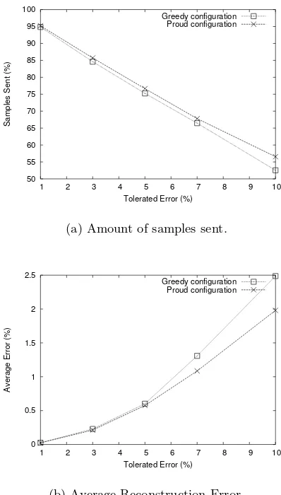
The results shown in Figs. 2 and 3, highlight the importance of a correct con-figuration of the scheme in order to achieve the best possible results. Moreover, according to the metric we decide to optimize, we can achieve very different re-sults. One possible configuration is to decide to always transmit as few samples as possible for every configuration of the maximum tolerated error. We will call this theGreedy configuration, and it could be implemented usingαequals to 1 and a lowupdate value, whenever the maximum tolerated error is low. When the maximum tolerated error grows we adopt a lowαand a highupdatevalue. Another option, namedProud configuration, is to always try to minimize the average reconstruction error. It can be implemented usingαalways equal to 1 and assigning high values for theupdateparameter, when the maximum toler-ated error is low. For higher maximum tolertoler-ated errors the updateparameter must be low. Fig. 4 shows the results obtained for these two configurations as a function of the tolerated error.

(9)

50 55 60 65 70 75 80 85 90 95 100

1 2 3 4 5 6 7 8 9 10

Samples Sent (%)

Tolerated Error (%) Greedy configuration

Proud configuration

(a) Amount of samples sent.

0 0.5 1 1.5 2 2.5

1 2 3 4 5 6 7 8 9 10

Average Error (%)

Tolerated Error (%) Greedy configuration

Proud configuration

[image:9.595.202.401.106.456.2]

(b) Average Reconstruction Error.

Fig. 4. Results from the ideal configurations.

4 Conclusion

This paper introduces and analyzes an event-driven field-estimation scheme. The scheme exploits the fact that not all the collected samples result in useful information. Therefore, we reduce the number of samples sent to the sink and, as a consequence, the energy consumption in the network.

(10)

scheme configuration must take into account the two metrics simultaneously. The results show that a significant increase in the estimation quality can be achieved in expense of a slightly smaller gain. A configuration aiming to optimize the average reconstruction error results in much smaller errors, achieving a gain a little smaller than the gain achieved by a Greedy configuration.

In the future, we intend to analyze the impact of the network losses on the results and to develop an adaptive configuration mechanism to ensure the achievement of the best possible results.

References

1. I. F. Akyildiz, W. Su, Y. Sankarasubramaniam, and E. Cayirci, “Wireless sensor

networks: a survey,”Computer Networks, vol. 38, pp. 393–422, 2002.

2. S. Tilak, N. B. Abu-Ghazaleh, and W. Heinzelman, “A taxonomy of wireless

micro-sensor network models,”ACM Mobile Computing and Communications

Re-view (MC2R), 2002.

3. A. Kumar, P. Ishwar, and K. Ramchandran, “On distributed sampling of smooth

non-bandlimited fields,” inInformation Processing In Sensor Networks - IPSN’04,

apr 2004, pp. 89–98.

4. G. P. Pottie and W. J. Kaiser, “Wireless integrated network sensors,”

Communi-cations of the ACM, vol. 43, no. 5, pp. 51–58, may 2000.

5. R. Willett, A. Martin, and R. Nowak, “Backcasting: adaptive sampling for sensor

networks,” in Information Processing In Sensor Networks - IPSN’04, apr 2004,

pp. 124 – 133.

6. M. Rahimi, R. Pon, W. J. Kaiser, G. S. Sukhatme, D. Estrin, and M. Sirivastava,

“Adaptive sampling for environmental robotics,” in IEEE International

Confer-ence on Robotics & Automation, apr 2004, pp. 3537–3544.

7. M. A. Batalin, M. Rahimi, Y.Yu, D.Liu, A.Kansal, G. Sukhatme, W. Kaiser, M.Hansen, G. J. Pottie, M. Srivastava, and D. Estrin, “Towards event-aware adap-tive sampling using static and mobile nodes,” Center for Embedded Networked Sensing - CENS, Tech. Rep. 38, 2004.

8. I. Lazaridis and S. Mehrotra, “Capturing sensor-generated time series with quality

guarantees,” in International Conference on Data Engineering (ICDE’03), mar

2003.

9. H. Chen, J. Li, and P. Mohapatra, “Race: Time series compression with rate

adap-tivity and error bound for sensor networks,” in IEEE International Conference

on Mobile Ad-hoc and Sensor Systems - MASS 2004, oct 2004.

10. D. O. Cunha, R. P. Laufer, I. M. Moraes, M. D. D. Bicudo, P. B. Velloso, and O. C. M. B. Duarte, “A bio-inspired field estimation scheme for wireless sensor

networks,”Annals of Telecommunications, vol. 60, no. 7-8, 2005.

11. M. Weiser and J. S. Brown, “The coming age of calm technolgy,” in Beyond

calculation: the next fifty years. Copernicus, 1997, pp. 75 – 85.

12. Universidade de S˜ao Paulo,Departamento de Ciˆencias Exatas, LCE ESALQ