Growth
A Dissertation
Presented to the Faculty of Economics
of
Universidad del Rosario
in Candidacy for the Degree of
Doctor of Philosophy in Economics
by:
IADER GIRALDO SALAZAR
Dissertation Director:
DR. Fernando Jaramillo Mejía
I am deeply appreciative of the numerous people who have supported my work and continually
encouraged me throughout the writing of this dissertation. Without their time, thoughtful feedback
and patience I would not have been able to complete this dissertation.
First of all, I wish to express my gratitude to my supervisor, Fernando Jaramillo Mejia PhD, for
his invaluable role as both a teacher and advisor. In particular, I sincerely appreciate his astute advice
and continual encouragement.
I would like to thank Thierry Verdier for his advice during my internship at the Paris School of
Economics; his pertinent recommendations have contributed to a great extent to the development
of this research. In addition, I wish to thank Hubert Kempf, Matthieu Crozet and Cecilia
García-Peñalosa, all of whom were generous with their time during my stay in Paris and when listening to
this thesis and providing me with various clear suggestions.
I would also like to thank the professors of the Faculty of Economics at the Universidad del Rosario
and the participants of the di¤erent seminars in which the articles that comprise this thesis were …rst
exposed; the resulting recommendations have signi…cantly improved the development of the present
dissertation.
Finally, I would like to thank my wife and my family for their patience and comprehension during
1 Introduction 3
2 Productivity, Demand and the Home Market E¤ect. 5
2.1 Introduction . . . 5
2.2 The Model . . . 8
2.2.1 Closed Economy . . . 10
2.3 Open Economy . . . 13
2.3.1 Producer . . . 15
2.4 The Home Market E¤ect . . . 15
2.5 Comparative Statics . . . 20
2.5.1 Variations in Population Size . . . 21
2.5.2 Variations in Relative Income . . . 21
2.5.3 Productivity . . . 23
2.5.4 Variations in Productivity and Supernumerary Income . . . 31
2.6 Conclusions . . . 33
2.7 Appendices . . . 34
2.7.1 Appendix 1 . . . 34
3 The Implications of International Trade on Economic Growth. 39 3.1 Introduction . . . 39
3.2 The Model . . . 42
3.2.1 Equilibrium in a Closed Economy . . . 44
3.3 Open Economy . . . 46
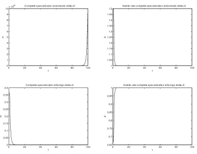
3.3.1 Complete Specialization . . . 52
3.3.2 Welfare . . . 55
3.5 Appendices . . . 60
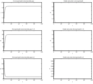
3.5.1 Appendix 1: Properties of the dynamic function of the net productivity gap (propositions 1 and 2) . . . 60
3.5.2 Appendix 2: The relation between equilibrium and asymptote . . . 64
4 Catching up with the "Joneses", the Home Market E¤ect and Economic Growth. 69 4.1 Introduction . . . 69
4.2 The Model . . . 72
4.3 Habit Speci…cation . . . 74
4.3.1 Producer . . . 75
4.4 Open Economy . . . 77
4.4.1 The Dynamic Implications of Habits . . . 80
4.4.2 The Dynamic Implications of Productivity . . . 83
4.5 The Dynamic in Productivity and Habits . . . 85
4.6 Welfare . . . 89
4.7 Conclusions . . . 92
4.8 Appendices . . . 92
4.8.1 Appendix 1 . . . 92
4.8.2 Appendix 2 . . . 93
Introduction
At present, we are witnessing globalization as a truly worldwide phenomenon. Trade agreements
among di¤ering countries, a reduction in trade costs, the mobility of production factors, the free ‡ow
of information and so on are all proof of the present day era of globalization. Countries are trading with
one another more and more every day and the e¤ects of international trade on economies represent a
central discussion in all economic spheres.
In spite of increasing trade around the world and the promotion of globalization by multilateral
organisms such as WTO and IMF, the e¤ects of international trade are not yet clear. Economics
liter-ature concerning the e¤ects of international trade on economic growth and welfare remains ambiguous
in terms of both theoretical models and empirical research. The present thesis tries to contribute to
the theoretical debate surrounding the e¤ects of dynamic international trade, focusing in particular on
the implications for economic growth, welfare and changes in the preferences of individuals.
This dissertation consists of three articles that double as chapters. In the …rst chapter I develop
an international trade model with the Home Market E¤ect, with di¤erences in income and
productiv-ity between countries and sectors. The inclusion of non-homothetic preferences allows the inclusion
of an original channel in the determination of international trade e¤ects, the demand composition.
The model allows for the identi…cation of static e¤ects of international trade through three main
de-terminants: population size, productivity levels and demand composition. Interactions among these
channels determine the trade e¤ects in terms of industrialization and the welfare of the countries that
trade.
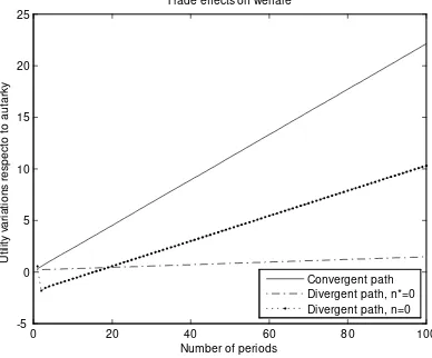
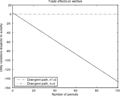
In the second chapter I analyze international trade e¤ects on economic growth. I consider an
endoge-nous economic growth model in an open economy with the Home Market E¤ect and non-homothetic
preferences. The implications of such modelling allow for an understanding of the heterogeneity of
part-convergence. Nevertheless, welfare can improve or decline after trade depending on convergence or
divergence in the income levels of the countries.
Finally, in the third chapter I consider a model of dynamic international trade in order to analyze the
e¤ects of international trade on the preferences of the agents and the implications for economic growth.
The model used is based on the Home Market E¤ect with external habit formation (catching up with the
"Joneses") and learning by doing in production. I …nd that the historical composition of consumption
within the countries determines industrialization levels after trade. The consumption habits of the
countries converge at the same level and composition shows the interrelation of consumption preferences
under trade. In spite of this convergence in consumption preferences, income levels may converge or
diverge among trade partners depending on the historical composition of consumption, supernumerary
income and productivity levels. The added e¤ect of convergence in the habits of consumption and
convergence or divergence in income levels generates di¤erent results for the welfare levels of countries
after trade, sometimes where the autarky is strictly preferred to trade.
This thesis proceeds as follows. Each chapter corresponds to an article. Every article contains an
introduction that references the literature review and presents some stylized facts about the speci…c
topic of each article. After the introduction, each article outlines the fundamentals of the model, the
Productivity, Demand and the
Home Market E¤ect.
2.1
Introduction
In an increasingly globalized world, bilateral and multilateral trade agreements occur more and more
frequently and do so among a larger variety of countries. Relationships between developed countries in
the European Union, the ascent of the BRIC countries (Brazil, Russia, India and China) in the world
market, and treaties between developed and developing countries, such as NAFTA, are becoming more
frequent. Within this context, a study of the e¤ects of international trade on well-being is of great
relevance. New trade theory and the performance of countries newly liberalized for world trade suggest
the importance of certain questions, such as, why are trade e¤ects di¤erent between countries and what
are the main variables that determine whether trade e¤ects are positive or negative?
In this article, we consider the aforesaid questions through a general equilibrium model of bilateral
trade with Home Market E¤ect (HME). In contrast to the standard literature of HME (Krugman
1980,1991, etc.), we introduce additional mechanisms by which trade increases or decreases Gross
Domestic Product (GDP) and well-being. This allows us to identify and analyze the most suitable trade
partners for an economy. Indeed, where non-homothetic preferences are at play, income di¤erences
between countries and di¤erences in productivity between sectors and between countries contribute to
the structure of demand inside each country. At the same time, in a model with HME, demand acts
over the e¤ects of trade liberalization on welfare and the industrialization of countries.
The model proposed herein analyses interactions between supply-side variables, like productivity,
mechanisms through which HME acts: population size, demand composition and levels of
productiv-ity. The consequences of international trade in terms of industrialization - as evident under positive
transportation costs - can be analyzed through the interplay of these three mechanisms. In fact, this
article shows that population size, demand structure and productivity levels determine the level of
in-dustrialization generated after international trade. In addition, we discuss the e¤ects of international
trade on welfare, which are positive whenever the global market of manufacturing increases after trade.
Traditional models of international trade focus on the supply side. In contrast, the new theory
of international trade, particularly that of Krugman (1980), takes into account the e¤ects of demand
on trade. The Home Market E¤ect establishes that the market size of a closed economy determines
its trade patterns and industrial development. This is an important factor that is …rst mentioned by
Linder (1961). This approach has allowed for the identi…cation of agglomeration and dispersion e¤ects
generated by trade, which show the positive and negative e¤ects of international trade on economic
performance, depending on the size of the market of each economy. Helpman and Krugman (1985).
The HME was …rst proposed by Corden (1970) and then extended by way of formal changes in a
seminal article by Krugman (1980). Further modi…cations have mainly been carried out by the same
author and presented in Helpman and Krugman (1985). The literature surrounding HME focuses on
population size as a demand element in determining patterns of trade and the industrial distribution
of countries, showing transportation costs as the crucial variable. Although this literature does not
exclude the possibility of additional mechanisms, it does not give su¢cient importance to these and
assumes the size of the country as being the only channel through which demand determines trade
patterns.
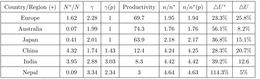
The traditional HME suggests that the most densely populated countries concentrate the
produc-tion of manufacturing internaproduc-tionally. However, in contrast with reality, China and India would have
bene…ted the most from trade relations at the international level. In particular, China and India have
populations 4.32 and 3.95 times larger than that of the United States respectively.1 However, trade between these countries has not allowed full specialization in the manufacturing industry for the former
examples (as predicted by the traditional HME), and much less any specialization in the other sectors
for a commercial counterpart.
In the presence of HME, the number of agents in an economy is a fundamental variable in
determin-ing trade patterns and the distribution of industrial production among countries that trade. However,
there are additional variables that complement this, and which therefore contribute to the …nal e¤ects
of international trade on GDP. Income and competitiveness di¤erentials determine the composition of
demand for countries, but these variables are shelved in HME standard modeling because this theory
assumes homothetic preferences. With the inclusion of the variables analyzed in our model, the size
of the market for industrial goods is limited by both the number of agents that comprise it and the
ability to generate demand in relation to their commercial counterpart.
The importance of the components of demand can be justi…ed by Engel’s law (Engel 1857), which
establishes that the income elasticity of demand for food is less than one (Banks, Blundell, and Lewbel,
1997). Accordingly, the higher an agent’s income, the lower the proportion of food spending. There
is a solid empirical bibliography that con…rms this law (Hamilton 2001, Banks, Blunder and Lewbel,
1997; etc. ). Consumer surveys about individual consumer spending in the United States show that
spending on food in 1946 was to the order of 24% of total consumption, while in 2011 it was only
7% (Bureau of Labor Statistics, 2014). This relationship is important in an international context due
to the heterogeneity in income levels between countries. Indeed, in terms of per capita the level of
income in the ninth decile of the distribution of countries is 72 times higher than in the …rst.2 This element, clearly di¤erentiated, has direct consequences for the patterns of demand in each country.
The countries with low levels of income must have a structure of demand mainly concentrated in vital
consumer goods. In contrast, countries with higher levels of income principally demand manufactured
goods. The higher the level of income, the higher the demand for manufactured items like cars,
computers, cell phones and so on. Mitra and Trindade (2005); Bohman and Nilsson (2007); Dalgin,
Mitra and Trindade (2008).
This article is based on empirical evidence regarding the importance of the composition of demand
in patterns of trade and speci…c specializations within countries (Markusen 1986; Dalgin, Mitra and
Trindade 2008). This evidence shows the presence of HME between di¤erent partner countries and
the interactions among supply and demand elements (Davis and Weinstein 1996; Davis, Hanson and
Weinstein 2003; Xiang 2004). Indeed, Yu (2005) shows the di¤erentiated e¤ects of HME after
includ-ing symmetrical transportation costs for both goods and di¤erences in the elasticity of substitution.
Chung (2006) shows the importance of demand composition in the determination of HME. Crozet and
Trionfeti (2008) show the non-linearity of HME. Huang and Huang (2011) demonstrate the possibility
of reversing HME with a technological advantage in production, based on a sample of six types of
industry. Indeed, the evidence supports the importance of building a good indicator of HME.
Less conclusive estimates about the presence of HME, such as Davis (1998) and Antweile and Tre‡er
(2002), reveal the presence of additional channels that are not taken into account by the traditional
model. Even the lack of a robust HME e¤ect may be due to the omission of key channels in the
determination of the structure of demand and thus due to the omission of key explanatory variables.
The most common procedure for including the determinants of demand in international trade
models entails the incorporation of non-homothetic preferences. Generally, the model assumes a utility
2Alan Heston, Robert Summers and Bettina Aten, Penn World Table Version 7.1, Center for International
function with a minimum consumption of vital goods (agricultural). After exceeding this threshold
of survival, income di¤erentials change the level of demand for manufactured goods in each country,
thus relating the composition of demand in each region to income levels. Furthermore, the addition of
di¤erences in productivity between countries allows us to consider the e¤ects of technological change
on income and prices, and as a consequence of the composition of demand and competitiveness in
each nation. This strategy is used by Stokey (1991) and Matsuyama (2000) in a product cycle model
with a North-South asymmetrical countries scenario. Zweimuller (2000) and Foellmi and Zweimuller
(2006) also use the same procedure to link the distribution of income to the composition of demand
and economic growth.
The e¤ects of trade between symmetric countries (North-North or South-South), as well as
asym-metric countries (North-South), can be studied by the model proposed herein. In addition, studying
HME through di¤erent channels gives robustness to empirical exercises that seek to establish the
pres-ence of HME in international trade. Indeed, when it is only the population size that is included in an
econometric exercise, there exists a bias due to omitted variables. The model shows that the inclusion
of additional variables that determine the structure of demand, such as productivity among countries
and among sectors, di¤erences in income and the composition of the population, allow for a more
robust analysis of the e¤ects of HME in relation to international trade.
This article consists of six sections, including the introduction. The second section presents the
characteristics of the model, the third shows the e¤ects of an open economy, the fourth exposes the
alternative HME in the model, the …fth presents comparative statics, and the sixth section concludes.
2.2
The Model
We start from the basic structure of the theory of the Home Market E¤ect, as presented by Krugman
(1980), but we break the homothetic preferences assumption and add the Stone-Geary utility function.
In addition, di¤erences in productivity between sectors and between countries are used.
We assume the presence of two regions, domestic and foreign ( ),3 independent of size. There are two types of good: homogeneous(X), which represents agricultural goods and presents constant returns to scale in production, and heterogeneous (Y), which represents manufactured goods and exhibits increasing returns to scale in production. The varieties of heterogeneous good are horizontally
di¤erentiatedà laDixit-Stiglitz, and the …rms in this sector maximize their bene…ts under monopolistic competition. Labor (L) is the only existing factor of production and is mobile among sectors but immobile among countries.
With the idea of modeling the e¤ects of demand composition on the internal market in a simple
way, we use the Chung (2006) strategy. This assumes that the number of people consuming di¤ers
from the number of people producing; countries have the same amount of labor (L=L ), but their populations(N andN )may be di¤erent. So it is supposed that domestic households o¤er one unit of work for each resident(N= L=L), while foreign households o¤er (1), meaning(N = L ).4
Intuitively, captures the demographic and redistribution factors that a¤ect the relative demand
for diversity goods in comparison to homogeneous goods. According to this modi…cation, it is possible
to interpret as the proportion of the population that earns an income.
The consumption side assumes that all households demand goods and that they symmetrically
demand each variety of heterogeneous good (Y). Households in both countries have the same non-homothetic utility function.
U = (X X) Y1 (2.1)
WithY =
n
X
i=1
yi
!1
,0< <1; n= number of varieties consumed (2.2) Where X is the minimum consumption (of survival) of the homogeneous good,5 and X is the consumption of this same good beyond the threshold of survival. Y is the aggregate consumption of allnvarieties of heterogeneous good andyi is the consumption of theith variety.
Both goods use the same factor of production, namely labor. The production of homogeneous
goods, and all varieties of the heterogeneous sector, is performed with the same function of production
in both countries. The homogeneous goods sector has the following production function:
Qx=LxAx (2.3)
In equilibrium it should be equal to added demand for this good.
N X =Dx=Qx=LxAx (2.4)
Where Qx is the aggregate production of a homogeneous good, Dx is the aggregate demand for
the homogeneous good,Lx is the amount of labor used in the production of this good, andAx is the
productivity in this sector. The cost function for the heterogeneous goods sector is given by:
li=
Ay
+ Qi
Ay
=
Ay
+ Di
Ay
i= 1;2:::n whereDi=N yi (2.5)
WhereQi andDi are, respectively, the aggregate supply and demand of thei-th variety,li is the
amount of labor used in the production of each variety, andAyis productivity in this sector. Moreover,
and are the parameters of …xed costs and variable costs, respectively.
4 >1
5This consumption is equal for all countries, indicating that everybody needs the same minimum consumption of food
Finally, the full-employment condition is assumed, meaning that:
L=LX+LY =
DX
AX
+
n
X
i=1
(
Ay
+ Di
Ay
) (2.6)
2.2.1
Closed Economy
Consumer
Agents maximize their utility function (2.1) subject to the budget restriction. With the aim of
intro-ducing di¤erences in the incomes of agents, as di¤erentiated by Chung (2006), this model di¤erentiates
between members of the household who work and those who only consume. It is assumed that in one
of the countries each worker supports additional agents that only consume; they are part of the total
population but not of the employed population, and they do not receive any income. The population
is proportional to the number of employees,N = L:6.
M axU= (X X) Y1 s.t. PxX+PyY =
w
(2.7)
After having been normalized by the total population (N), the consumer maximization program de…nes the optimal quantities demanded of good X, and the aggregate demand of all varieties of heterogeneous goodY.
Y =1
Py
w
PxX (2.8)
X =
P x w
PxX +X (2.9)
WherePxis the price of a homogeneous good,Py is the price index of heterogeneous goods, which
is an aggregate price of each variety’s price. The optimization process de…nes the demand of each
variety of heterogeneous good, which is determined by aggregate spending on such goods, the price of
each varietyi, and the sum of the price of all thenvarieties.
yi=
p
1 1
i (1 ) w PxX
P 1
y
(2.10)
Where Py = n
X
i=1
pi 1
! 1
(2.11)
Py is the index price for the heterogeneous good that is found fromyi and its implications on the
aggregate demand for heterogeneous goods (2.2). This index is established as an aggregate of prices
of di¤erent varieties, weighted by the degree of substitutability between them.
Producer
In the production of homogeneous goods there exists a competitive environment, thus implying an
equilibrium with zero pro…t. At the same time, the price of the homogeneous good has been established
as a numeraire. As a result, the wages(w)in the homogeneous goods sector are exogenous and equal to productivity:
Px= 1 =
w Ax
(2.12)
A direct consequence of the last equation is that the per capita income, in terms of homogeneous
goods, is completely determined for productivity in this sector and the dependence factor : wL
N = AxL
N = Ax
(2.13)
For the heterogeneous goods sector, the presence of a large number of varieties implies that the
price decision of each …rm has virtually no e¤ect on the marginal utility of income. Therefore, the
function of demand for each variety (2.10) is such that the price elasticity of demand (y;p) of each of
the varieties is constant and exogenous:
y;p=
@yi
@pi
pi
yi
(2.14)
y;p=
1
(1 ) (2.15)
In the monopolistic competition scenario for which the production of such goods is inscribed, there
is an explicit relationship between price elasticity and marginal cost, which maximizes bene…ts for the
…rms that produce some of the varieties of heterogeneous good.
pi 1
1
y;p
= Cmg (2.16)
p = pi=
w Ay
(2.17)
From (2.17), the price of each variety is de…ned by parameters, being constant for all varieties.
Inserting the prices into the zero bene…ts condition, determined by the free entry and exit of …rms, it
is possible to …nd the production of each variety of heterogeneous good, which is equal to the total
demand for each variety.
i = pDi
Ay
+ Di
Ay
w= 0 (2.18)
D = Di=
(1 ) (2.19)
In the last equation, it is possible observe that the quantity demanded of and produced for each
variety is independent of the productivity rate and country size. As is typical in models with
Finally, from the full-employment condition (2.6) one can obtain the number of varieties of
hetero-geneous good present in this economy.
Ly = n
X
i=1 Ay
+ Di
Ay
(2.20)
n = Ly(1 )Ay (2.21)
The amount of labor used in the heterogeneous sector is the total available workforce minus the
quantity used in the production of homogeneous goods.
Ly = L Lx (2.22)
Ly = L N +
(1 )
Ax
X (2.23)
Replacing (2.23) and (2.21) it is possible to …nd the number of varieties as a function of the
parameters of the model, the amount of the available productivity factor, and the productivity within
each sector of the economy.
n=
L N + 1
Ax X (1 )Ay
(2.24)
The Equation (2.24) can be rewritten in the following way:
nA = Ax X (1 )(1 )Ay Ax
N (2.25)
nA = (A
x X)(1 )(1 )
Ay
Ax
L
(2.26)
For the last equation (2.25), it can be noted that the number of varieties (n) produced in a country corresponds to its level of industrialization.7 Basically, this depends on three particular elements. First, the comparative advantages (Ay
Ax), de…ned by the ratio between the productivity of the two sectors of the economy. This ratio determines the competitiveness of a country, according to its
relative production advantages in one of the two sectors. Second, the population size of the country,
in the sense of the standard theory of HME. Third, the supernumerary income (Ax X), which
determines the purchasing power of workers in terms of heterogeneous goods. These elements persist
in the open economy and determine the e¤ects of international trade.
Additionally, the degree of industrialization that is determined by the number of varieties produced
7The level of industrialization can also be de…ned by the amount of labor available in the manufactured goods sector
in the manufacturing sector also determines welfare levels.
UA = (Ax
X) 0
@ (1 )
n 1 Ax Ay Ax X 1 A 1 (2.27)
UA = (1 )1
1
nA
(1 )(1 ) A
y
Ax 1
Ax
X (2.28)
The greater the degree of country industrialization, the greater the welfare. Similarly, the same
variables that determine the level of industrialization of a country a¤ect welfare levels. In summary, the
levels of productivity in the sector of manufactured goods, the population size and the supernumerary
income de…ne both the degree of industrialization of a country and its welfare.
2.3
Open Economy
In this section, we extend the model to an open economy scenario, which establishes the basis for the
HME model. There are two trading countries that di¤er in population size (N) and productivity in each of the sectors(Ax yAy).
Assuming costless international trade in the homogenous good (X),8 its price is equalized in the two countries. This price will be taken as a numeraire (Px=Px = 1). There are transportation costs
associated with the heterogeneous goods trade, which are modeled as "iceberg" transportation costs.
In particular, it is supposed that a portion of the transported goods arrives, while (1 ) is lost in
transit. Including this relationship of costs to prices in the international market, the prices of each
variety of heterogeneous good are as follows:
Domestic
8 < :
p=p
b
p =p
, Foreigner
8 < :
p =p
b
p= p
(2.29)
Therefore, the consumption of national varieties di¤ers from the varieties imported due to price
di¤erences. The representative home maximizing program is then modi…ed in relation to the varieties of
heterogeneous domestic and foreign goods.9 The aggregate consumption of varieties of heterogeneous good is no longer represented by (2.2), but it becomes an aggregate of both domestic and foreign
varieties that di¤er in priceY0
= Pni=1yi +
Pn
j=1yj
1
. Therefore, the budget constraint is now
de…ned by:
n
X
i=1
piyi+ n
X
i=1
b
pjyj (1 )
w
PxX (2.30)
8This is a simpli…ed assumption that is widely used (Helpman & Krugman 1985; Krugman 1991, etc.) and which
does not a¤ect the essential argument of the model.
9 L= 0 @ n X i=1
yi +
n X j=1 yj 1 A 1 n X i=1
piyi+
n X
i=1 c
pjyj (1 )
w
PxX
Whereyi is the demand for each domestic variety and yj is the demand for each foreign variety.
The budget restriction at the foreign level is symmetric to this.
As a result of the maximization, we …nd the ratio between the demand for domestic and foreign
varieties to be a function of the price ratio of these,
yj yi
= pi
b
pj
! 1
1
(2.31)
The local demand for each variety of heterogeneous domestic and foreign good (yiandyj),
result-ing from the maximization program of the domestic agent, is de…ned by the proportion of revenue
earmarked for heterogeneous goods demand and the price of each variety weighted by the addition of
the prices of all available varieties around the world.
yi =
p
1 1
i (1 ) w PxX
Pn
i=1p 1
i +
Pn
j=1pb 1
j
(2.32)
yj = p^
1 1
j (1 ) w PxX
Pn
i=1p 1
i +
Pn
j=1pb 1
j
(2.33)
The new basket of varieties available worldwide that enters into the aggregation of heterogeneous
goods Y0
, modi…es its index price, similarly a¤ecting the proportion of income available for the
con-sumption of such goods. Performing the same procedure as that used with the price index in a closed
economy, the free-trade index, depends on the price of existing domestic and foreign varieties of
het-erogeneous goods:
PY0 = 2 4 n X i=1 p 1 i + n X j=1 b p 1 j 3 5 1 (2.34)
Equation (2.31) is the ratio between the consumption of domestic and foreign varieties in terms of
the ratio between prices. In order to determine the world equilibrium we need to add the quantities of
the goods used for the transportation of products. The demand rate for foreign heterogeneous goods,
in terms of the domestic ( ) and corresponding rates for foreign goods ( ) is equal to:
= yj
yi
= pi
pi
1 1
1
(2.35)
= yi
yj = pi
pi
1 1
1
= pi
pi
1 1
1
(2.36)
After determining the ratio of demand for varieties among foreign and domestic varieties, one can
de…ne individual demand patterns for heterogeneous goods in each country, which are restricted by
and foreign heterogeneous goods are:
yi =
pi
PY0
1 1
(1 )
w P xX
PY0 !
(2.37)
yj = pbj
PY0
! 1
1
(1 )
w P xX
PY0 !
(2.38)
2.3.1
Producer
Using equations (2.37) and (2.38) it is easy to show that the elasticity of demand for exports is the
same as in a closed economy for heterogeneous goods (11 ). Therefore, transportation costs have no
e¤ect on the pricing policy of the …rm. This result shows that the domestic and foreign prices of each
variety of heterogeneous good remain the same as under autarky, in their respective local markets.
p= w
Ay
^ p = w
Ay (2.39)
Given the characterization of monopolistic competition in the market of heterogeneous goods, every
variety of this type of good is only produced by one …rm.10 The number of varieties produced in each region is determined in the …rst instance by productivity in this sector, the amount of labor force used
in the production of these goods (Ly andLy) and the model parameters.
n=Ly(1 )Ay ^ n =Ly(1 )Ay (2.40) With regard to the homogeneous good, the equalization of prices at the international level sets a
relationship of proportionality between the wages and agricultural productivity of both countries.
w=Ax and w =Ax (2.41)
In accordance with the equation (2.41), the per capita incomes, in terms of the homogeneous good,
are the same as in a closed economy.
wL N =
Ax
and w L
N = Ax
2.4
The Home Market E¤ect
The presence of increasing returns to scale in the production of heterogeneous goods, and transportation
costs generated for its trade at the international level, create an incentive to produce such goods in
the "biggest market", thus taking advantage of economies of scale and minimizing transportation costs
1 0The only way in which the results are modi…ed in relation to the closed economy is if the wages between countries
(Krugman 1980, 1991, etc.). In this sense, and according to the purposes of this article, the "largest
market" is not only determined by the number of agents in a country, but also by their productivity
and per capita supernumerary incomes. In other words, the demand e¤ect, through the purchasing
power and the level of competitiveness of the agents, constitutes a market.
Starting with two countries that possess the established features, aggregate demand for
heteroge-neous goods in each country is the sum of the domestic and foreign demand for this type of good, that
is, the domestic consumption of heterogeneous goods plus exports of these kinds of good (2.42 and
2.43).11
npD = n
n+ pp n
(1 ) w X N+ n
n+ pp n
(1 ) w X N (2.42)
n p D = n
p
p n+ n
(1 ) w X N+ n
p
p n+n
(1 ) w X N (2.43) Aggregate demand for heterogeneous goods in a closed economy, which is only determined by the
proportion of domestic spending dedicated to this type of good, is now determined by a combination
of variables regarding the economies that are trading. In particular: a) the proportion of spending on
such goods(1 ); (b) the demand rate among domestic and foreign varieties, that is, ultimately, a
price ratio (fractions depending on (nand )); (c) the supernumerary income of the agents; and (d) the total population. Additionally, the productivity in each of the two sectors plays a fundamental role in
the demand for such goods through the real income of workers. On the one hand, the productivity of
the homogeneous good sector determines wages, demarcating agents’ revenues and the costs of …rms,
while the productivity of the heterogeneous sector determines the price of each variety.
Solving (2.42) and (2.43) obtains the relationship between the number of varieties produced
domes-tically against those produced overseas as a measure of HME, which is determined by the interactions
between supply and demand elements that are additional to those presented in the traditional
ap-proach.
pn p n =
(Ax X)N(1 )
Ax X N (1 )
1 (1 )(
Ax X)N
(1 ) Ax X N
(2.44)
Equation (2.44) is a novel result in the theory of international trade with increasing returns to
scale. In the …rst instance, it is evident that the HME presented through the varieties rate of the
heterogeneous goods produced in each country depends on the same elements as its traditional version,
the parameter ( ), which mainly includes the e¤ects of the trade frictions, particularly transportation
costs. However, in equation (2.44) we identify other channels by which the ratio (n
n ), and therefore
HME, can be changed.
1 1Dis determined by the zero pro…t conditionD
The term between the brackets of equation (2.44) collects most of the di¤erent e¤ects evident in
this relationship. The …rst fraction of this term
Ax X
Ax X , corresponds to the relative supernumerary income, which is a direct consequence of the non-homothetic preferences assumption and relates to
the purchasing power of the agents. The second term corresponds to the relationship with population
sizes N
N , which shows the e¤ects of the ratio among the sizes of the markets, in the standard
form of HME. Finally, the last expressions in parentheses convey the degree of competitiveness of the
markets according to their productive advantages, weighted by existing trade frictions 11 . In
global terms, the expression re‡ects the relationship between the relative sizes of the demands of the
two countries, which is determined by population size, the purchasing power of agents and the degree
of competitiveness of these.
The disparity between( 6= )re‡ects the di¤erence in per capita income (Ax), which will modify the demand for heterogeneous goods in each country, a¤ecting the number of varieties of heterogeneous
goods produced in each region. This channel identi…es di¤erences in the purchasing power of the
residents of a market. It is hoped that countries with greater purchasing power demand a higher
proportion of heterogeneous goods, creating an incentive for the establishment of …rms in this market,
which will increase the number of varieties produced.
Variation in the productivity of both sectors is another channel through which international trade
can a¤ect the degree of industrialization of a country. Variations in productivity in the homogeneous
good sector alters wages, generating two contrary e¤ects within the economy that result in a
di¤eren-tiated aggregate e¤ect. The …rst is an expenditure e¤ect, which alters the level of revenue dedicated
to the purchase of heterogeneous goods. The second is a cost e¤ect, which changes the prices for each
variety of these goods. These two e¤ects act in opposite directions, and so the result of an increase
ofAx, in terms of the number of varieties produced, depends on the magnitude of each one of these
e¤ects. Furthermore, variations in the productivity of heterogeneous goods modify the prices of such
goods and thus the number of varieties in demand, leading to alterations in the number of varieties
produced in each country. Productivity within both sectors …gures strongly in the case of comparative
static, which is developed in the next section.
In order to simplify the initial analysis, equal productivity among the sectors of each country is
assumed (Ax = Ay = A), but it di¤ers between countries (A 6= A ). In this way, there exists a
scenario in which relative income and productivity vary between countries. The …nal e¤ects of trade
will therefore depend on the three fundamental channels described in this article, which produce HME:
assumptions presented for the general result (2.44) are veri…ed in the following equation:
n n =
(A X)N
(A X)N 1
1 1 (
A X)N
(A X)N
= Z 1
1 1 Z (2.45)
where
Z=
A X N
A X N (2.46)
This equation presents the e¤ects of the di¤erent channels on the HME through the number of
produced varieties of heterogeneous good. The Z variable in the equation (2.45) corresponds with the supernumerary income ratio (the centerpiece of this result, since it depends on the three channels
in question) and the ratio of population size. The Z variable collects the di¤erent channels in the model, so that supernumerary income is a¤ected by the country’s productivity levels, the dependence
factor ( ) and population size. Increased productivity or a reduced dependence factor increases per
capita income levels, creating a demand e¤ect. This in turn stimulates the production of more varieties
of heterogeneous good in the country with a higher income. This is so because it boosts the size of
demand, which allows it to exploit economies of scale. Countries with a greater supernumerary income,
as caused by any of the channels presented in this case, will then have a higher real income, which
increases the economic market size, directly a¤ecting the number of varieties of heterogeneous good
produced in the economy.12
In HME function (2.45), the interval of incomplete specialization, where both countries produce
two types of good, occurs when the(Z) variable belongs to the interval 1 ; 1
1 . The greater the transportation costs and the lower the economies of scale, the greater the range of incomplete
specialization. Outside this interval of the variable, the full specialization of the partners takes place.
A trade balance in the heterogeneous goods of a domestic country is obtained from the demands of
these goods from domestic and foreign countries.
T BY =
n
n+n (1 ) A
X N n
n+ n (1 ) A
X N (2.47) The behavior of the trade balance in the range of incomplete specialization depends on
exoge-nous variables (productivity, dependence factors, proportion of income devoted to spending on
het-erogeneous goods and transportation costs), and the number of varieties of hethet-erogeneous good
pro-duced in each country. When the countries have the same supernumerary income and population size
Z= (
A X)N
(A X)N = 1 , both produce the same number of varieties of heterogeneous good, presenting equilibrium in the trade balance of manufacturing. Out of equilibrium, the performance of the trade
1 2In the annex we show that, even when international trade reduces the degree of industrialisation in the countries,
balance depends on the number of varieties produced in each country (2.48), which is directly de…ned
by the relationship between the supernumerary incomes of the countries and population size (2.45).
The country with a higher per capita income will produce more varieties than the other, and will
experience a trade balance surplus in heterogeneous goods at this interval.
T BY =
A X (1 )L 1
1 n+n (n n ) (2.48)
T BY > 0,n > n (2.49)
IfZ > 11 , the trade between the two countries will involve a full specialization in heterogeneous goods domestically, and in homogeneous goods overseas. On the other hand, ifZ < 1 , the trade between the two countries will take on a full specialization in heterogeneous goods overseas, and in
homogeneous goods domestically. The more similar (di¤erent) the traded countries are (Zt1) in
terms of population size, income and productivity, the higher (lower) the probability of incomplete
specialization, intra-industry trade (inter-industry trade).
The e¤ects of(Z)on the number of varieties produced in each country can be determined analyti-cally and show a positive relation. The country with a higher income will be the largest producer of
heterogeneous goods within a bilateral trade relationship, with positive transportation costs:
d(nn)
dZ =
1 12
1 1 (
A X)N
(A X)N
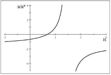
2 >0 given <1 (2.50) Given the characteristics of the HME function (2.45), this can be represented in a graph, as shown
Figure 1: Population size, supernumerary income and HME
The graph is similar to the traditional HME. It shows the variable Z and the channels involved, while de…ning the number of varieties produced by each country. Located on the right of the asymptote
are the cases of complete specialization in heterogeneous goods on domestic production after trade
implementation. Similarly, the points to the left of the intercept demarcate the overseas cases of
complete specialization for such goods. The interval between the intercept and the asymptote is the
area of incomplete specialization and illustrates the case in which both countries are equal (Z = 1) and produce the same number of varieties.
Is important to highlight that the HME is determined by theZvariable and not only by population size, as in traditional models. It shows the importance of the demand composition in the results of
the trade. More than country size, economic market size is key in the sense of the purchasing power of
agents, which determines the consequences of international trade on the degree of industrialisation for
countries that trade. International trade increases industrial production in relation to autarky levels
if the relative supernumerary income is su¢cently greater in relation to the transportation cost.
On the other hand, via this same model it is possible to determine the trade implications for welfare.
The relationship between utility under an open economy and autarky is such that it will only depend
on the number of varieties to which the country has access after and before trade,ceteris paribus.
U UA
= n
nA
+n 1
nA
!(1 )(1 )
(2.51)
The outcome in terms of welfare depends on two e¤ects: the …rst is the number of varieties
pro-duced domestically after trade, in relation to the number propro-duced under autarky, and the second is
the number of additional varieties that are accessed after trade in relation to those available under
autarky. These two e¤ects can go in the same direction or in opposite directions, depending on whether
specialization exists or not, and the impact of trade on the production of heterogeneous goods.
How-ever, using the de…nitions about the number of varieties produced under autarky and under trade, we
…nd that welfare is better under trade than under autarky. This means that in the static scenario
exposed in this model, trade is strictly preferred to autarky.
U UA
= 1 + 1
(1 )(1 )
>1 (2.52)
2.5
Comparative Statics
From (2.44), it is possible to generate the di¤erent comparative statics that enable the identi…cation of
the di¤erent channels through which HME may occur after trade liberalization, and they demonstrate
2.5.1
Variations in Population Size
Assume the absence of a homogeneous good, that the population is equal to the number of workers, that
productivity is equal between the countries, and that transportation costs are positive ( = 0; L=N ,
X= 0and >0). With these assumptions we achieve the classic results obtained by Krugman (1980), who presents the relationship between population sizes as determinant of the number of varieties of
heterogeneous good produced in each country. HME is determined by the population size of each
country (Z = N
N ). The graphic representation of this scenario is illustrated in …gure 1, where HME
is determined by the values that take the variableZ.
n n =
Z
1 Z =
N N
1 N
N
(2.53)
Given dNdZ >0 , the larger a country in terms of population, the greater the number of varieties of heterogeneous good being produced. It is clear that the size of the population, as Krugman (1980)
states, is an important channel in the determination of HME, but it is not the only element that
comes into this determination because, as we shall see later on, both the purchasing power and level
of productivity in each of the sectors complement the channels through which the size of a market
becomes a determinant of the type of product that one country trades (HME).
2.5.2
Variations in Relative Income
Assume the existence of a homogeneous good with a minimum level of consumption 6= 0andX >0 , the population di¤ers from the number of workers in each economy (L6=N; withN = L), and the other variables are equal between countries, while HME is obtained from the relative demand of the
market. Given the above assumptions, per capita income di¤erentials determine the structure of
the demand and so delimit the heterogeneous good varieties produced in each country after trade
liberalization.
According to the hypothesis, the prices of every variety are the same in both countries, therefore
= = 1 . By de…nition N = L, assuming = 1 for domestic and > 1 for foreign, the relationship presented in (2.44) is de…ned in the following way:
n n =
Z 1
1 Z 1 with Z=
A X N
A X N (2.54)
(2.54) has the same functional form of the standard HME, which in this case is presented through
other channels and is represented in …gure 1. TheZ variable determines the complete or incomplete specialization of countries at the same intervals set out in the general case. There is a point where the
income is equal for both countries ( = ), and they therefore produce the same number of varieties
in terms of heterogeneous goods exhibits a particular behavior that is determined by the number of
varieties produced in each country (2.55), which in turn is determined by the level of income of each
region. Therefore, the country with higher levels of income (fewer ) will have a trade balance surplus
in manufacturing.
T BY =
(A X) (1 )L
1 n+n (n n ) (2.55)
T BY > 0,n > n ^ n > n , > (2.56)
In equation (2.50) we show that d(nn)
dZ >0, and so the e¤ect of the increases in the variable , which
contains the di¤erentials of per capita income against a foreign partner, is positive.13 Accordingly, the higher the per capita income of countries, the greater the number of varieties produced.
dz d =
Ax X X
Ax X 2
!
>0 if Ax> X (2.57)
Proposition 1 : In a world characterized by the presence of homogeneous and heterogeneous goods, where productivity is equal among countries and among sectors, and each country has a di¤erent level of supernumerary income, after trade the country with the higher relative income (less ) will produce a greater number of varieties in the heterogeneous goods sector. At the same time, the country with a higher level of income will have a trade surplus in this sector and its industrial production will be greater than under autarky.
The result presented in proposition 1 goes in the same direction as the issues raised in the in-troduction and as that of the argumentation of the overall result. Countries with higher levels of
supernumerary income spend the bulk of their income on elaborate items, which increases market size
for this type of good, and so it becomes attractive to establish …rms in this sector of production in
order to take advantage of economies of scale.
In terms of welfare, the results can be obtained by comparing levels of utility under autarky and
in an open economy (2.52). The welfare levels under an open economy are superior to those under
autarky because of the greater number of varieties available to agents. International trade increases
the varieties available around the world, which allows for an increase in the levels of utility for both
countries in relation to their situation under autarky.
1 3This is true so long as worker remuneration is higher than the survival consumption of the agricultural good; this is
2.5.3
Productivity
Total productivity
Equalizing the labor-force sizes of the countries, and assuming equality between the population and
the number of employees(N =L), productivity di¤erences among countries are entered. Productivity di¤ers between countries but productivity among sectors is equal for each country (Ax = Ay = A
and A 6= A ). Incorporating the assumptions above into the general equation (2.44), the following expression is reached, which is also represented in …gure 1:
n n =
Z 1
1 1 Z con Z =
A X
A X (2.58)
Di¤erences in productivity, as they are shown, allow for the inclusion of supply and demand e¤ects
within the relationship of the varieties of heterogeneous goods. The demand e¤ect dominates through
di¤erences in income, and can even generate a complete specialization via productivity di¤erentials.
The external position of each economy in the range of incomplete specialization behaves similarly to
the previous case. When the productivity factor is equal between countries, they produce the same
amount of varieties and achieve a trade balance for di¤erentiated goods. However, when productivity
di¤ers, that trade balance depends on the number of varieties produced (2.59), as directly de…ned by
the productivity factor. A more productive country will have a positive trade balance in heterogeneous
goods.
T BY =
A X (1 )L 1
1 n+n (n n ) (2.59)
T BY > 0,n > n ^ n > n ,A > A (2.60)
Given d(nn)
dZ >0, the e¤ect of variations in the productivity factor on the number of varieties of
heterogeneous goods produced in each country can be determined analytically, showing their direct
relationship. In this way, the most productive country within the trade relationship will be the largest
producer of heterogeneous goods.14
d(z)
dA =
1
A X >0 si A > X (2.61)
Proposition 2 : Bilateral trade in countries that only di¤er in their productivity factors, these being equal between sectors, means that the country with higher productivity produces a superior number of varieties of heterogeneous good in relation to its trade partner and its autarky production. At the same time, the country with higher productivity will have a trade surplus in the manufacturing sector.
Proposition 2 goes in the same direction mentioned above. The productivity channel, such as it arises in this case, raises the supernumerary income in the more productive country, creating a demand
e¤ect that leads to an increase in the market of heterogeneous goods, making the establishment of …rms
within this sector in the said country attractive. Countries with high levels of productivity will have
high levels of income, which increases the number of varieties among the heterogeneous goods produced.
The current result exposes agglomeration and dispersion e¤ects posed by the standard theory
of HME, but via changes in productivity. However, the demand e¤ect is much higher, resulting in
the agglomeration e¤ect dominating the dispersion. More productive countries will generate better
remunerations for workers (income e¤ect), while the cost e¤ect is cancelled due to a reduction in this
via productivity in equal magnitude to the increase in wages. Therefore, a more productive country
will have a greater weight of heterogeneous goods in the composition of the individual demand, leading
the producers of such goods to becoming established in this market in order to exploit economies of
scale.
In terms of welfare, the result compared with autarky is determined in the same way by (2.52).
The increase in global demand for heterogeneous goods generates greater varieties, which raises the
levels of welfare for countries with respect to their situation in a closed economy.
Comparative advantage in heterogeneous goods
Detailing a little more regarding the implications of changes in productivity, this is a singular case in
which there are variations between regions and sectors. Initially, the e¤ects of productivity variations
in the heterogeneous goods sector are examined, when these di¤er between countries and within the
homogeneous goods sector, ceteris paribus. In a formal wayAy 6= Ay 6=Ax; Ax =Ax, then z = 1:
De…ning y = Ay
Ay as the relationship pertaining to productivity in the manufacturing sector. The inclusion of these assumptions in (2.44) generates the following output:
n n =
y H
1 1
y 1
1
1 1
y 1 H
(2.62)
where
H= 1
1 1
y 1
1
1 1
y 1
(2.63)
As in the previous cases, the functional form is maintained, although the variables involved are
clearly di¤erent. H de…nes the positive range of the function, which presents the possibility of incom-plete specialization
1 1
y 1 ; 1 1 1
y 1
!
Figure 2: HME and the competitiveness factor
The trade balance of the heterogeneous goods in this interval is again determined by the number
of varieties produced in each country, and also by the relationship with productivity in this sector
(2.64). Similarly, at the point where both economies have the same productivity, they produce the
same number of varieties and present an external equilibrium in this sector.
T BY = (
1 1
y
1 1
y )
1 (1 ) Ax X N
1
1 1
y 1 1
1 1
y 1
(2.64)
T BY > 0,n > n , y >1 (2.65)
Equation (2.62), presents the competitiveness factorH and the relationship between productivities ( y;which represents the price ratio) as determinants of HME. The way in which these variables relate can be veri…ed analytically using the following expressions.
@n n
@H =
y 1 +
2 1
1
1 1
y 1 H
2 >0 (2.66)
@ n n
@ y
=
H
1 1
y 1
1
1 1
y 1 H
+
1 1
1 1
y 1 +
1 1
y 1 H2 2
2
1 H
1
1 1
y 1 H
Competitiveness factor H and the relationship between productivities among the heterogeneous goods y are directly related to the quotient of varieties produced between countries. The e¤ects of variations in the productivity of heterogeneous goods are channeled via prices of this type of good. In
this way, both supply and demand e¤ects are presented. The …rst reduces costs for …rms in the more
productive country, after producing the same with less labor, increasing the number of varieties o¤ered
by the added open market. The second, the price e¤ect, increases the number of varieties in demand,
given the lower price of each. Finally, the di¤erentiation in the factor of competitiveness with respect
to the relationship for productivity is:
dH d y =
1 1
2+ 1
y 1 + y1 1 2 2
1 1
y
1
1 1
y 1
2 >0 (2.68)
The result of (2.68), related to (2.66), determines the aggregate e¤ect of costs, which is presented
as positive due to increased e¢ciency in manufacturing output. At the same time, the e¤ect of the
relationship between productivities is direct (2.67).15 E¤ects in the same direction create a positive aggregate e¤ect. The more productive the country in the manufacturing sector, the greater the number
of varieties that it produces.
d n n
d y
>0,H2 1 ; 1
1 (2.69)
Proposition 3 : Trade between countries that only di¤er in productivity regarding the heterogeneous goods sector means that the country with greater productivity in this sector produces a higher number of varieties of heterogeneous good in relation to its trade partner and its autarky production. The greater the productivity in the heterogeneous goods sector, the greater the number of varieties produced. The e¤ect on the trade balance of the more productive country is also positive.
This proposition contributes to a delimiting of the e¤ects of productivity as the channel of
compet-itiveness among economies that trade. Thus productivity in the heterogeneous goods sector directly
a¤ects the size of the market and may strengthen HME. The result is clear that in the interest interval,
where there exists incomplete specialization, the agglomeration e¤ect dominates, so a direct
relation-ship between comparative advantage in the heterogeneous goods sector and the number of varieties
produced in the country is present.
Similar to the above cases, it is possible to determine the e¤ects on welfare by comparing the levels
of utility between an open economy and autarky. In this case, the expression that determines these
e¤ects takes into account the implications of di¤erences in productivity on the relative prices of the
domestic varieties with respect to the foreigner. U UA = 0 B
@nn
A + n y 1 nA 1 C A
(1 )(1 )
= 0 @ 1 2 1 1 1 1 y 1 1 A
(1 )(1 )
>1 (2.70) The welfare levels under an open economy are superior to those under autarky because of the
greater number of varieties available to agents.
Comparative advantage in homogeneous goods
The other way to see particular di¤erences in productivity between countries and between regions is
through productivity in the homogeneous goods sector. Maintaining all other variables equal, countries
only di¤er in productivity in relation to homogeneous goods, which in turn di¤ers from productivity in
relation to heterogeneous goods Ax6=Ax6=Ay andAy =Ay . De…ning x=AAxx as the relationship between productivity for homogeneous goods in the two countries obtains the following result:
n n =
1 x
"
Ax X Ax x X 1 1 1 x 1 1 1 1 x 1 ! 1 1 x 1 # 1 1 1 1
x AAxx X
x X 1 1 1 x 1 1 1 1 x 1 ! = 1 x ZH 1 1 x 1 1 1 1 1 x ZH (2.71)
The functional form persists andZHde…nes the interval of incomplete specialization 1 1
x 1 ; 1
1 1 1 x
!
through di¤erent channels. This result is presented in …gure 3, which shows a graphic representation
Figure 3: HME supernumerary income and competitiveness factor
This time, the behavior of the trade balance in this interval is given by the number of varieties
produced in each country and the relationship between productivities for homogenous goods (wages)
(2.72). Similarly, there is a case of balanced trade in this sector when the countries have the same
level of productivity in the sector in question.
T BY =
1 A
x X (1 )L
1 1
x 1 n+n x1
( 1 1 x n 1 1
x n ) (2.72)
T BY > 0,
n n >
2 1
x (2.73)
The last term in (2.71) incorporates the factor of competitiveness among countries H, the super-numerary income ratioZ, and the ratio of productivity between countries in the homogeneous goods sector x= Ax
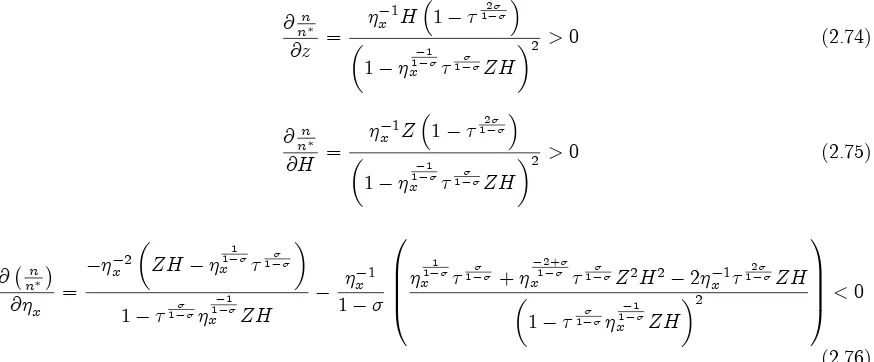
Ax, as determinants of HME. This expression allows for an analytical veri…cation of how these determinants relate to the ratio of varieties between countries.
@ n n
@z =
1 x H 1
2 1
1
1 1
x 1 ZH
2 >0 (2.74)
@ n n
@H =
1 x Z 1
2 1
1
1 1
x 1 ZH
2 >0 (2.75)
@ n n
@ x =
2 x ZH 1 1 x 1 1 1 1 1 x ZH 1 x 1 0 B B B @ 1 1
x 1 +
2+ 1
x 1 Z2H2 2 1
x 2 1 ZH 1 1 1 1 x ZH 2 1 C C C A<0
(2.76)
Competitiveness factor H and relative supernumerary income Z relate directly to the ratio of varieties produced between countries, while the relationship of productivity in the homogeneous goods
sector xrelates indirectly. However, ending the di¤erentiation:
dz d x = 0 B @ Ax 2
x(Ax X)
Ax
x X
2
1 C
A>0 if Ax> X (2.77)
dH d x = 1 1 1
x 1 +
2+ 1
x 1 2 x1
2 1 1 1 1 x 1
2 <0 (2.78)
The result presented in (2.77), combined with (2.74), allows for the identi…cation of the aggregate
factor. Similarly, the result (2.78), related to (2.75), determines the aggregate e¤ect of costs, which is
negative by the increase in the remuneration of labor.
The results in this case are ambiguous, since two contrary e¤ects coexist. On the one side there
is an income e¤ect through the increase in wages that increases the demand, and therefore raises
the proportion of the heterogeneous goods demanded. This e¤ect from the demand side increases the
number of varieties produced in the more productive country. On the other side is the cost e¤ect, which
arises from increases in wages after increases in productivity, and rises one to one the remuneration
of labor, thus reducing the number of varieties produced in the more productive country because of
the high costs of production and the tendency to specialize in the production of homogeneous goods.
This ambiguity in the relationship shows the presence of the agglomeration and dispersion e¤ects of
the HME referenced above, and presents the existence of a trade-o¤ between them, allowing any …nal
result depending on the magnitudes of each.
d n n
d x = @ n
n
@ x
( )
+@
n n
@Z dZ d x
(+)
+@
n n
@H dH d x
( )
Proposition 4 : The trade between countries that only di¤er in their productivity in the homogeneous goods sector generates opposite e¤ects on the number of varieties of heterogeneous good produced in each country, the aggregate outcome being dependent on the magnitude of the e¤ects presented. On the one side, the demand e¤ect stimulates the production of more varieties given increases in wages, but on the other side, the cost e¤ect reduces the number of varieties produced because the cost of production is higher.
Proposition 4 contributes, from an alternative angle, to the delimitation of a competitiveness channel as a determinant of the market size of the economies that trade. The presence of contrary
e¤ects adds ambiguity to the aggregate result, presenting the result that productivity in this sector
reinforces the HME when the agglomeration e¤ect dominates; or, on the contrary, it weakens when
the dispersion e¤ect is predominant.
To reduce ambiguity in the results, a simulation was executed in order to determine the values of the
parameters within which the dispersion or agglomeration e¤ect dominates. Table 1 shows the values
that the parameters must take for the agglomeration e¤ect to dominate the dispersion e¤ect. The
…rst row presents the values that should take the transportation cost parameter if we use the standard
values of substitution elasticity among varieties. Similarly, the second row presents the values that
should take the substitution elasticity parameter among varieties if we use the standard values of
transportation costs.
d(n
n )
d x >0 = 0:4 ^ <0:025 = 0:8 ^ <0:38 = 0:9 ^ <0:59 Standard Values d(n
n )
Table 1: Parameter values, agglomeration dominates dispersion e¤ect
These results suggest that the dispersion e¤ect dominates the agglomeration e¤ect in situations
with economic sense in the value of the parameters. The agglomeration e¤ect would only dominate
in cases in which the transportation costs or the elasticity of substitution between varieties were
extraordinarily high, cases in which international trade is possibly not established. This result justi…es
the fact that some industries will migrate to developing countries with low levels of productivity and
wages. This is the case for industries in China or India, where an increase in the number of …rms is
due more to low-wage labor than to a large and e¤ective demand for heterogeneous goods. When the
dispersion e¤ect dominates, it is possible to produce far from the larger markets and assume the costs
of international trade, due to the low production costs of less productive countries.
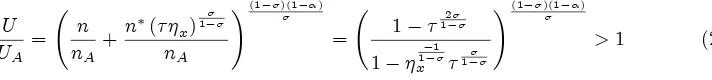
As in other cases, the e¤ect on welfare in relation to levels of utility could be set under autarky.
The following expression exhibits this relationship, including di¤erentials in productivity in the
homo-geneous goods sector.
U UA
= n
nA
+n ( x)1
nA
!(1 )(1 )
= 1
2 1
1
1 1
x 1
!(1 )(1 )
>1 (2.79)
Similar to the previous cases, the e¤ect on welfare is always positive in relation to autarky when
the size of the global market for heterogeneous goods increases after trade. Regardless of the outcome
of the trade in relation to the industrialization of countries, welfare increases along with the number
of varieties to which people have access.
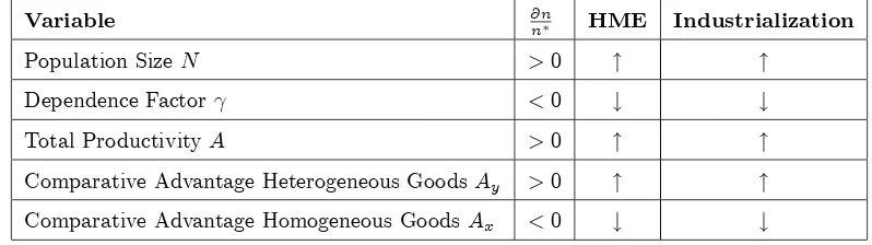
Comparative statics summary
The comparative statics show how the di¤erent variables a¤ect the number of varieties produced in each
country. This is evidence of the existence of di¤erent channels in HME determination. Interactions
among channels from the demand and supply side determine HME in a distinct way. The next
table summarizes the e¤ects of each determinant on HME. The …rst column shows the relationship
between each determinant and the quotient of varieties produced for each country (the sign of the
…rst di¤erentiation). The second column presents what happens to the HME when two countries start
to trade and each variable becomes greater at the domestic rather than foreign level. Finally, the