5
Designing and Operating a
Warehouse
5.1
Introduction
Warehouses are facilities where inventories are sheltered. They can be broadly classi-fied intoproduction warehousesand DCs. This chapter deals with warehouse design and operation, with an emphasis on DCs. In the following, aproductis defined as a type of good, e.g. wine bottles of a specific brand. The individual units are called items(orstock keeping units(SKUs)). Acustomer order is made up of one or more items of one or more products.
Flow of items through the warehouse. Warehouses are often used not only to provide inventories a shelter, but also to sort or consolidate goods. In a typical DC, the products arriving by truck, rail, or internal transport are unloaded, checked and stocked. After a certain time, items are retrieved from their storage locations and transported to an order assembly area. In the simplest case (which occurs frequently in CDCs (see Chapter 1)), the main activity is the storage of the goods. Here, the merchandise is often received, stored and shipped in full pallets (all one product) and, as a result, material handling is relatively simple (see Figure 5.1). In the most complex case (which occurs frequently in RDCs (see Chapter 1)) large lots of prod-ucts are received and shipments, containing small quantities of several items, have to be formed and dispatched to customers. Consequently, order picking is quite com-plex, and product sorting and consolidation play a mayor role in order assembly (see Figure 5.2).
Ownership of the warehouses. With respect to ownership, there are three main typologies of warehouses.Company-owned warehousesrequire a capital investment in the storage space and in the material handling equipment. They usually represent the least-expensive solution in the long run in the case of a substantial and constant demand. Moreover, they are preferable when a higher degree of control is required to ensure a high level of service, or when specialized personnel and equipment are
Article A
Receiving
Holding
Picking
Shipping
Figure 5.1 The flow of items through the warehouse; the goods are received and shipped in full pallets or in full cartons (all one product).
Article B
Holding
Picking Receiving
Batch forming
Packaging
Shipping Article A
Holding
Picking Receiving
Article C
Holding
Picking Receiving
Figure 5.2 The flow of items through the warehouse; the goods are received in full pallets or in full cartons (all one product) and shipped in less than full pallets or cartons.
Holding 15%
Handling 50% Receiving
17%
Shipping 18%
Figure 5.3 Common warehouse costs.
Finally,leased warehouse spaceis an intermediate choice between short-term space rental and the long-term commitment of a company-owned warehouse.
Warehouse costs. The total annual cost associated with the operation of a ware-house is the result of four main activities: receiving the products, holding inventories in storage locations, retrieving items from the storage locations, assembling customer orders and shipping. These costs depend mainly on the storage medium, the stor-age/retrieval transport technology and its policies. As a rule, receiving the incoming goods and, even more so, forming the outgoing lots, are operations that are diffi-cult to automate and often turn out to be labour-intensive tasks. Holding inventories depends mostly on the storage medium, as explained in the following. Finally, picking costs depend on the storage/retrieval transport system which can range from a fully manual system (where goods are moved by human pickers travelling on foot or by motorized trolleys) to fully automated systems (where goods are moved by devices under the control of a centralized computer). Common warehouse costs are reported in Figure 5.3.
5.1.1
Internal warehouse structure and operations
The structure of a warehouse and its operations are related to a number of issues:
• the physical characteristics of the products (on which depends whether the products have to be stored at room temperature, in a refrigerated or ventilated place, in a tank, etc.);
• the number of products (which can vary between few units to tens of thousands);
Storage zone Receiving zone
Shipping zone
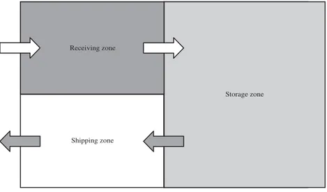
Figure 5.4 Warehouse with a single receiving zone and a single shipping zone.
Typically, in each DC there are (see Figure 5.4)
• one or more receiving zones(each having one or more rail or truck docks), where incoming goods are unloaded and checked;
• astorage zone, where SKUs are stored;
• one or moreshipping zones(each having one or more rail or truckdocks), where customer orders are assembled and outgoing vehicles are loaded.
The storage zone is sometimes divided into a largereserve zonewhere products are stored in the most economical way (e.g. as a stack of pallets), and into a small forward zone, where goods are stored in smaller amounts for easy retrieval by order pickers (see Figure 5.5). The transfer of SKUs from the reserve zone to the forward zone is referred to as areplenishment. If the reserve/forward storage is well-designed, the reduction in picking time is greater than replenishment time.
5.1.2
Storage media
Receiving zone
Reserve zone
Forward zone
Shipping zone
Figure 5.5 Warehouse with reserve and forward storage zones.
Figure 5.6 Block stacking system.
3.5 m wide. Instead, as explained in the following, inautomated storage and retrieval systems(AS/RSs), racks are typically 10–12 m tall and aisles are usually 1.5 m wide (see Figure 5.8). Finally, in the third case, items are generally of small size (e.g. metallic small parts), and are kept in fixed or rotating drawers.
5.1.3
Storage/retrieval transport mechanisms and policies
Figure 5.7 Rack storage.
Figure 5.8 An AS/RS.
Picker-to-product versus product-to-picker systems. The picking operations can be made
• by a team of human order pickers, travelling to storage locations (picker-to-productsystem);
• by an automated device, delivering items to stationery order pickers (order-to-pickersystem).
y
x
Figure 5.9 Item retrieval by trolley.
are delivered to storage locations by automated devices which are usually restricted to a single aisle. Inwalk/ride and pick systems(W/RPSs), pickers travel on foot or by motorized trolleys and may visit multiple aisles (see Figure 5.9).
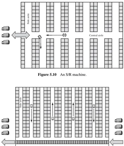
The most popular order-to-picker systems are the AS/RSs. An AS/RS consists of a series of storage aisles, each of which is served by a single storage and retrieval (S/R) machine or crane. Each aisle is supported by apick-up and delivery station customarily located at the end of the aisle and accessed by both the S/R machine and the external handling system. Therefore, assuming that the speedsvx andvy along
the axesxandy(see Figure 5.10) are constant, travel timestsatisfy the Chebychev metric,
t =max
x vx
,y vy
,
wherexandyare the distances travelled along thex- andy-axes.
AS/RSs were introduced in the 1950s to eliminate the walking that accounted for nearly 70% of manual retrieval time. They are often used along with high racks and narrow aisles (see Figure 5.11). Hence, their advantages include savings in labour costs, improved throughput and high floor utilization.
Unit load retrieval systems. In some warehouses it is possible to move a single load at a time (unit load retrieval system), because of the size of the loads, or of the technological restrictions of the machinery (as in AS/RSs). In AS/RSs, an S/R machine usually operates in two modes:
• single cycle: storage and retrieval operations are performed one at a time;
Side aisle
Central aisle
Figure 5.10 An S/R machine.
Side aisle
Figure 5.11 Item storage and retrieval by an AS/RS and a belt conveyor.
There exist systems in which it is possible to store or pick up several loads at the same time (multi-command cycle).
Strict order picking versus batch picking. In multiple load retrieval systems, customer orders can be assigned to pickers in two ways:
• each order is retrieved individually (strict order picking);
• orders are combined into batches.
5.1.4
Decisions support methodologies
Warehouses are highly dynamic environments where resources have to be allocated in real-time to satisfy customer orders. Because orders are not fully known in advance, design and operational decisions are affected by uncertainty. To overcome the inher-ent difficulty of dealing with complex queueing models or stochastic programs, the following approach is often used.
Step 1. A limited number of alternative solutions are selected on the basis of expe-rience or by means of simple relations linking the decision variables and simple statistics of customer orders (the average number of orders per day, the average number of items per order, etc.).
Step 2. Each alternative solution generated in Step 1 is evaluated through a detailed simulation model and the best solution (e.g. with respect to throughput) is selected.
5.2
Warehouse Design
Designing a warehouse amounts to choosing its building shell, as well as its layout and equipment. In particular, the main design decisions are
• determining the length, width and height of the building shell;
• locating and sizing the receiving, shipping and storage zones (e.g. evaluating the number of I/O ports, determining the number, the length and the width of the aisles of the storage zone and the orientation of stacks/racks/drawers);
• selecting the storage medium;
• selecting the storage/retrieval transport mechanism.
The objective pursued is the minimization of the expected annual operating cost for a given throughput, usually subject to an upper bound on capital investment.
In principle, the decision maker may choose from a large number of alternatives. However, in practice, several solutions can be discarded on the basis of a qualitative analysis of the physical characteristics of the products, the number of items in stock and the rate of storage and retrieval requests. In addition, some design decisions are intertwined. For instance, when choosing an AS/RS as a storage/retrieval transport mechanism, rack height can be as high as 12 m, but when traditional forklifts are used racks must be much lower. As a result, each design problem must be analysed as a unique situation.
5.2.1
Selecting the storage medium and the storage/retrieval
transport mechanism
The choice of storage and retrieval systems is influenced by the physical characteristics of the goods, their packaging at the arrival and the composition of the outgoing lots. For example, in a single storage zone warehouse, palletized goods are usually stocked on racks if their demand is high enough, otherwise, stacks are used. Automated systems are feasible if the goods can be automatically identified through bar codes or other techniques. They have low space and labour costs, but require a large capital investment. Hence, they are economically convenient provided that the volume of goods is large enough.
5.2.2
Sizing the receiving and shipment subsystems
The receiving zone is usually wider than the shipping area. This is because the incom-ing vehicles are not under the control of the warehouse manager, while the formation of the outgoing shipments can be planned in order to avoid congesting the output stations.
Determining the number of truck docks
Goods are usually received and shipped by rail or by truck. In the latter case, the number of docksnDcan be estimated through the following formula,
nD=
dt qT ,
where d is the daily demand from all orders, t is the average time required to load/unload a truck, q is the truck capacity, andT is the daily time available to load/unload trucks.
Sintang is a third-party Malaysian firm specialized in manufacturing electronic devices. A new warehouse has been recently opened in Kuching. It is used for storing digital satellite receivers, whose average daily demand isd =27 000 units. Outgoing shipments are performed by trucks, with a capacity equal to 850 boxes. Since the average time to load a truck ist =280 min and 15 working hours are available every day, the warehouse has been designed with the following numbernDof docks:
nD=
27 000×280 850×900 =10.
5.2.3
Sizing the storage subsystems
storage and retrieval times become uselessly high. This could decrease throughput or increase material handling costs.
Determining the capacity of a storage area
The size of a storage area depends on the storage policy. In a dedicated storage policy, each product is assigned a pre-established set of positions. This approach is easy to implement but causes an underutilization of the storing space. In fact, the space required is equal to the sum of the maximum inventory of each product in time. Letnbe the number of products and letIj(t), j=1, . . . , n, be the inventory level of
itemj at timet. The number of required storage locationsmdin a dedicated storage
policy is
md=
n
j=1
max
t Ij(t). (5.1)
In arandom storage policy, item allocation is decided dynamically on the basis of the current warehouse occupation and on future arrival and request forecast. Therefore, the positions assigned to a product are variable in time. In this case the number of storage locationsmris
mr=max
t n
j=1
Ij(t)md. (5.2)
The random storage policy allows a higher utilization of the storage space, but requires that each item be automatically identified through a bar code (or a similar technique) and a database of the current position of all items kept at stock is updated at every storage and every retrieval.
In aclass-based storage policy, the goods are divided into a number of categories according to their demand, and each category is associated with a set of zones where the goods are stored according to a random storage policy. The class-based storage policy reduces to the dedicated storage policy if the number of categories is equal to the number of items, and to the random storage policy if there is a single category.
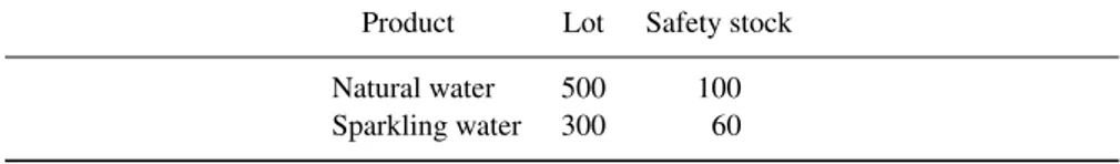
Potan Up bottles two types of mineral water. In the warehouse located in Hangzhou (China), inventories are managed according to a reorder level policy (see Chapter 4). The sizes of the lots and of the safety stocks are reported in Table 5.1. Inventory levels as a function of time are illustrated in Figures 5.12 and 5.13. The company is currently using a dedicated storage policy. Therefore, the number of storage locations is given by Equation (5.1):
md=600+360=960.
The firm is now considering the opportunity of using a random storage policy. The number of storage locations required by this policy would be (see Equation (5.2))
Table 5.1 Lots and safety stocks (both in pallets) in the Potan Up problem.
Product Lot Safety stock
Natural water 500 100
Sparkling water 300 60
I(t)
t 100
350 600
Figure 5.12 Inventory level of natural mineral water in the Potan Up problem.
60 210 360 I(t)
t
Figure 5.13 Inventory level of sparkling mineral water in the Potan Up problem.
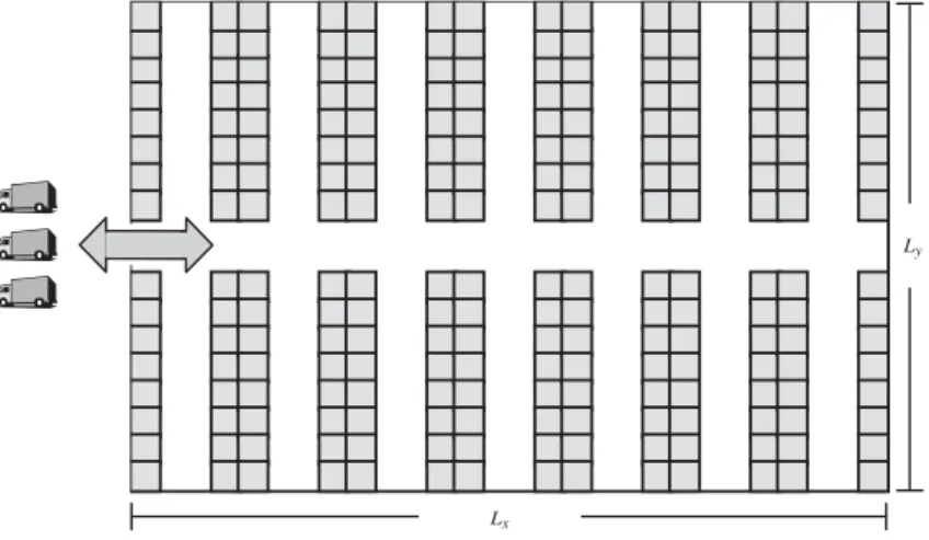
Determining length, width and height of a storage zone
Lx
Ly
Figure 5.14 A traditional storage zone.
height of the racks/stacks/drawers is determined by the storage technology. Therefore, the sizing decision amounts to calculating the length and the width. Let mbe the required number of stocking positions;αxandαythe occupation of a unit load (e.g.
a pallet or a cartoon) along the directionsxandy, respectively;wxandwy, the width
of the side aisles and of the central aisle, respectively;nz the number of stocking
zones along thez-direction allowed by the storage technology;vthe average speed of a picker. The decision variables arenx, the number of storage locations along the
x-direction, andny, the number of storage locations along they-direction.
The extensionLxof the stocking zone along the directionxis given by the following
relation,
Lx =(αx+12wx)nx,
where, for the sake of simplicity,nxis assumed to be an even number. Similarly, the
extensionLyis
Ly=αyny+wy.
Therefore, under the hypothesis that a handling operation consists of storing or the retrieving a single load, and all stocking points have the same probability of being accessed, the average distance covered by a picker is: 2(Lx/2+Ly/4)=Lx+Ly/2.
Hence, the problem of sizing the storage zone can be formulated as follows.
Minimize
(αx+12wx)
nx
v +
αyny+wy
2v (5.3)
subject to
nxnynzm (5.4)
where the objective function (5.3) is the average travel time of a picker, while inequal-ity (5.4) states that the number of stocking positions is at least equal tom.
Problem (5.3)–(5.5) can be easily solved by relaxing the integrality constraints on the variablesnxandny. Then, inequality (5.4) will be satisfied as an equality:
nx=
m nynz
. (5.6)
Therefore,nxcan be removed from the relaxed problem in the following way.
Minimize
(αx+12wx)
m nynzv +
αyny+wy
2v (5.7)
subject to
ny0.
Since the objective function (5.7) is convex, the minimizernycan be found through the following relation:
d d(ny)
(αx+12wx)
m nynzv +
αyny+wy
2v
ny=ny
=0.
Hence,
ny=
2m(αx+12wx)
αynz
. (5.8)
Finally, replacingnyin Equation (5.6) by thenyvalue given by Equation 5.8,nxis
determined:
nx=
mαy
2nz(αx+12wx)
. (5.9)
Consequently, a feasible solution (n¯x,n¯y) is
¯
nx= nx and n¯y= ny.
Alternatively, a better solution could be found by settingn¯x = nx(orn¯y= ny),
provided that Equation (5.4) is satisfied.
Reserve zone Forward zone
Figure 5.15 Warehouse with a reserve/forward storage system.
speed of a trolley is 5 km/h. Using Equations (5.8) and (5.9), variablesnxandnyare
determined:
nx=
780×1.05
2×4×(1.05+32.5)=6.05,
ny=
2×780×(1.05+32.5)
1.05×4 =32.25.
Assumingn¯x =6 andn¯y=33, the total number of storage locations turns out to be
792, whileLx= [1.05+(3.5/2)]×6=16.8 m andLy=1.05×33+4=38.65 m.
Sizing a forward area
In a reserve/forward storage system (see Figure 5.15), the main decision is to deter-mine how much space must be assigned to each product in the forward area. In principle, once this decision has been made, the problem of determining the length, width and height of the pick-up zone should be solved. However, since each picking route in the forward area usually collects small quantities of several items, at every trip a large portion of the total length of the aisles is usually covered (see Figure 5.15). Hence, the dimensions of the pick-up zone are not critical and can be selected quite arbitrarily.
If the number of items stored in the forward area increases, replenishments are less frequent. However, at the same time the extension of the forward area increases and, consequently, the average picking time also goes up.
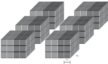
Let (see Figure 5.16)nbe the number of products,othe average number of orders per time period;d the average number of orders in a batch;oj, j =1, . . . , n, the
average number of orders containing productj;uj, j =1, . . . , n, the average number
of items of productjin an order;vthe average speed of a picker in the forward area;
wj
mj
Figure 5.16 Storage locations assigned to an itemj, j=1, . . . , n.
length and per time period;fj, j = 1, . . . , n, the fixed cost of a replenishment of
productj;gj, j =1, . . . , n, the variable cost for replenishing a unit of productj;
wj, j=1, . . . , n, the length of a portion of aisle occupied by an item of productj;
mj, j = 1, . . . , n, the number of items of productj that can be stored in an aisle
position. The decision variables are the number of aisle positionssj, j =1, . . . , n,
assigned to each productj.
The contribution of productj, j=1, . . . , n, to the cost of picking items from the reserve area is
c1j(sj)=h
(o/d)wjsj
v , (5.10)
whereo/drepresents the average number of batches picked up per time period (i.e. the average number of times a picker passes in front of a position per time period);wjsj
is the total length of the portion of aisle assigned to the productj,[(o/d)wjsj]/v
represents the average time spent during a time period by the picker because of productj.
The contribution of productj, j =1, . . . , n, to the average cost per time period of replenishing the forward area is
c2j(sj)=fj
ujoj
mjsj +
gjujoj,
whereujojrepresents the average demand per time period of productj, whilemjsj
is the number of storage locations assigned to productj, and(ujoj)/(mjsj)is the
average number of resupplies of productj per time period.
The portion of the space and equipment costs due to productj, j=1, . . . , n, is
Moreover, let sjmin andsjmax, j=1, . . . , n, be lower and upper bounds on the number of positions of productj, respectively. The problem of sizing the forward area can be modelled as follows.
Minimize
n
j=1
[c1j(sj)+c2j(sj)+c3j(sj)] (5.11)
subject to
sminj sj sjmax, j =1, . . . , n, (5.12)
sj 0, integer, j =1, . . . , n, (5.13)
where the objective function (5.11) is the sum of the costs due to the various prod-ucts, while constraints (5.12) impose lower and upper bounds on the number of aisle positions assigned to each itemj, j=1, . . . , n.
Problem (5.11)–(5.13) can be decomposed intonsubproblems, one for each product
j, j =1, . . . , n, and solved by exploiting the convexity of the objective function.
Step 1. Determine the valuesj, j =1, . . . , n, that minimizes the total costcj(sj)=
c1j(sj)+c2j(sj)+c3j(sj)due to productj:
dcj(sj)
dsj
sj=sj
=0, j =1, . . . , n,
sj =
fjujoj
mj[howj/dv+kwj]
, j =1, . . . , n.
Sets¯j = sj, ifcj(sj) < cj(sj), otherwises= sj, j=1, . . . , n.
Step 2. Compute the optimal solutionsj∗, j=1, . . . , n, as follows:
s∗j =
smin
j , ifs¯j < sjmin,
¯
sj, ifsminj s¯j sjmax,
smax
j , ifs¯j > sjmax,
j =1, . . . , n.
The total length of the aisleswtotcan then be obtained by the following relation:
wtot=
n
j=1
wjsj∗. (5.14)
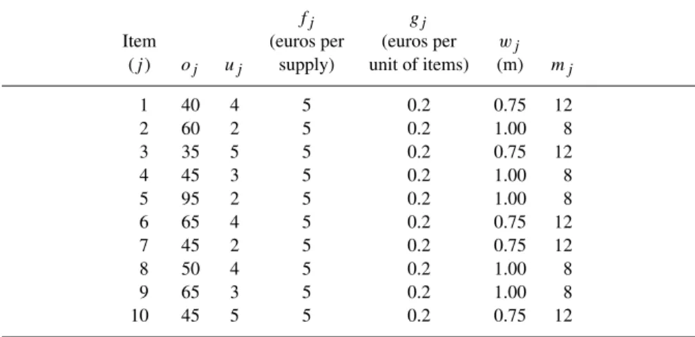
Table 5.2 Characteristics of the products at stock in the Wellen warehouse.
fj gj
Item (euros per (euros per wj
(j) oj uj supply) unit of items) (m) mj
1 40 4 5 0.2 0.75 12
2 60 2 5 0.2 1.00 8
3 35 5 5 0.2 0.75 12
4 45 3 5 0.2 1.00 8
5 95 2 5 0.2 1.00 8
6 65 4 5 0.2 0.75 12
7 45 2 5 0.2 0.75 12
8 50 4 5 0.2 1.00 8
9 65 3 5 0.2 1.00 8
10 45 5 5 0.2 0.75 12
Wellen is a Belgian firm manufacturing and distributing mechanical parts for numer-ical control machines. Its warehouse located in Herstal consists of a wide reserve zone (where the goods are stocked as stacks), and of a forward zone. At present 10 prod-ucts are stored (see Table 5.2). Then,o=400 orders per day,d =3 orders per lot,
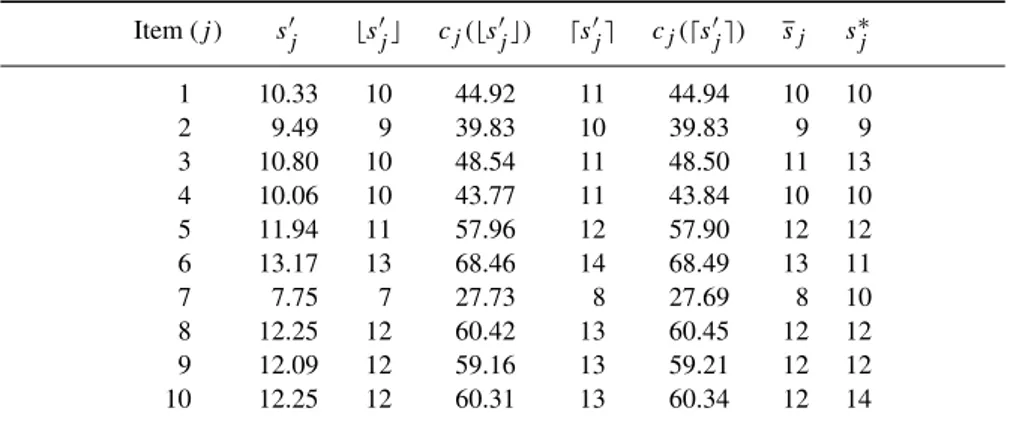
v=12 000 m per day,h=€75 per day, while the area and equipment cost per unit of aisle lengthkis assumed to be negligible. The minimum and the maximum number of positions for the various products are reported in Table 5.3. The number of positions
sj∗, j =1, . . . ,10, to be assigned to the different products in the forward zone can be obtained through the two-stage procedure previously described. The results are reported in Table 5.4. Consequently, the total lengthwtotof the aisles of the forward zone is equal to 98.5 m (see Equation (5.14)), while the workload is around 1.09 working days, so that at least two pickers are required.
5.3
Tactical Decisions
The main tactical decision consists of allocating products to space. In this section, the problem is modelled as a structured LP problem, namely, the classicaltransportation problem.
5.3.1
Product allocation
Table 5.3 Minimum and maximum number of aisle positions in the Wellen warehouse.
Item (j) sjmin sjmax
1 9 14
2 5 12
3 13 15
4 8 10
5 7 20
6 9 11
7 10 13
8 8 15
9 11 16
10 14 19
Table 5.4 Number of aisle positions in the forward zone of the Wellen warehouse.
Item (j) sj sj cj(sj) sj cj(sj) sj s∗j
1 10.33 10 44.92 11 44.94 10 10
2 9.49 9 39.83 10 39.83 9 9
3 10.80 10 48.54 11 48.50 11 13
4 10.06 10 43.77 11 43.84 10 10
5 11.94 11 57.96 12 57.90 12 12
6 13.17 13 68.46 14 68.49 13 11
7 7.75 7 27.73 8 27.69 8 10
8 12.25 12 60.42 13 60.45 12 12
9 12.09 12 59.16 13 59.21 12 12
10 12.25 12 60.31 13 60.34 12 14
allocation problem amounts to assigning each of themdstorage locations available to
a product. Letnbe the number of products;mj, j =1, . . . , n, the number of storage
locations required for productj (in a dedicated storage policy, relationnj=1mj
mdholds);R the number of I/O ports of the warehouse;pj r, j = 1, . . . , n, r =
1, . . . , R, the average number of handling operations on productj through I/O port
rper time period;trk, r=1, . . . , R, k=1, . . . , md, the travel time from I/O portr
and storage locationk.
Under the hypothesis that all storage locations have an identical utilization rate, it is possible to compute the costcj k, j =1, . . . , n, k =1, . . . , md, of assigning
storage locationkto productj,
cj k = R
r=1
pj r
mj
I/O port 2
I/O port 1 1 5 6 10 11 15 16 20 21 25 26 30 31 35 36 40
Figure 5.17 Warehouse of the Malabar company.
wherepj r/mjrepresents the average number of handling operations per time period
on productj between I/O portrand anyone of the storage locations assigned to the product. Consequently,(pj r/mj)trkis the average travel time due to storage location
kif it is assigned to productj.
Letxj k, j =1, . . . , n, k=1, . . . , md, be a binary decision variable, equal to 1 if
storage locationkis assigned to productj, 0 otherwise. The problem of seeking the optimal product allocation to the storage locations can then be modelled as follows.
Minimize
n
j=1
md
k=1
cj kxj k (5.16)
subject to
md
k=1
xj k =mj, j =1, . . . , n, (5.17) n
j=1
xj k 1, k=1, . . . , md, (5.18)
xj k∈ {0,1}, j =1, . . . , n, k=1, . . . , md, (5.19)
where constraints (5.17) state that all the items at stock must be allocated, while constraints (5.18) impose that each storage locationk, k=1, . . . , md, can be assigned
to at most one product.
It is worth noting that because of the particular structure of constraints (5.17) and (5.18), relations (5.19) can be replaced with the simpler nonnegativity conditions,
Table 5.5 Features of the products of the Malabar company.
Number of storages and retrievals per day in the Malabar warehouse
Storage
Item locations I/O port 1 I/O port 2
1 12 25 18
2 6 16 26
3 8 14 30
4 4 24 22
5 8 22 22
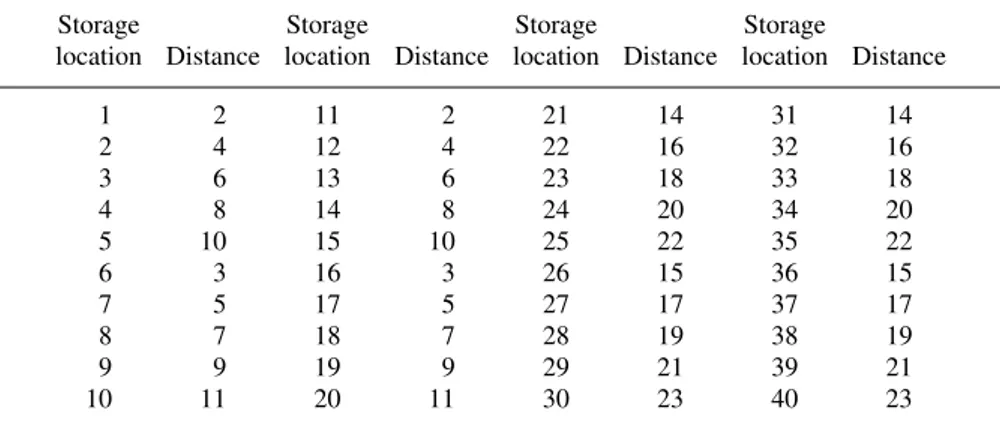
Table 5.6 Distance (in metres) between storage locations and I/O port 1 in the Malabar warehouse.
Storage Storage Storage Storage
location Distance location Distance location Distance location Distance
1 2 11 2 21 14 31 14
2 4 12 4 22 16 32 16
3 6 13 6 23 18 33 18
4 8 14 8 24 20 34 20
5 10 15 10 25 22 35 22
6 3 16 3 26 15 36 15
7 5 17 5 27 17 37 17
8 7 18 7 28 19 38 19
9 9 19 9 29 21 39 21
10 11 20 11 30 23 40 23
Table 5.7 Distance (in metres) between storage locations and I/O port 2 in the Malabar warehouse.
Storage Storage Storage Storage
location Distance location Distance location Distance location Distance
1 22 11 22 21 10 31 10
2 20 12 20 22 8 32 8
3 18 13 18 23 6 33 6
4 16 14 16 24 4 34 4
5 14 15 14 25 2 35 2
6 23 16 23 26 11 36 11
7 21 17 21 27 9 37 9
8 19 18 19 28 7 38 7
9 17 19 17 29 5 39 5
Table 5.8 Cost coefficientscj k, j=1, . . .5, k=1, . . . ,20, in the Malabar problem.
Assignment cost
Storage Product Product Product Product Product
locationk j=1 j=2 j=3 j=4 j=5
1 37.17 100.67 86.00 133.00 66.00
2 38.33 97.33 82.00 134.00 66.00
3 39.50 94.00 78.00 135.00 66.00
4 40.67 90.67 74.00 136.00 66.00
5 41.83 87.33 70.00 137.00 66.00
6 40.75 107.67 91.50 144.50 71.50
7 41.92 104.33 87.50 145.50 71.50
8 43.08 101.00 83.50 146.50 71.50
9 44.25 97.67 79.50 147.50 71.50
10 45.42 94.33 75.50 148.50 71.50
11 37.17 100.67 86.00 133.00 66.00
12 38.33 97.33 82.00 134.00 66.00
13 39.50 94.00 78.00 135.00 66.00
14 40.67 90.67 74.00 136.00 66.00
15 41.83 87.33 70.00 137.00 66.00
16 40.75 107.67 91.50 144.50 71.50
17 41.92 104.33 87.50 145.50 71.50
18 43.08 101.00 83.50 146.50 71.50
19 44.25 97.67 79.50 147.50 71.50
20 45.42 94.33 75.50 148.50 71.50
since it is knowna priori that there exists an optimal solution of problem (5.16)– (5.18), (5.20) in which the variables take 0/1 values.
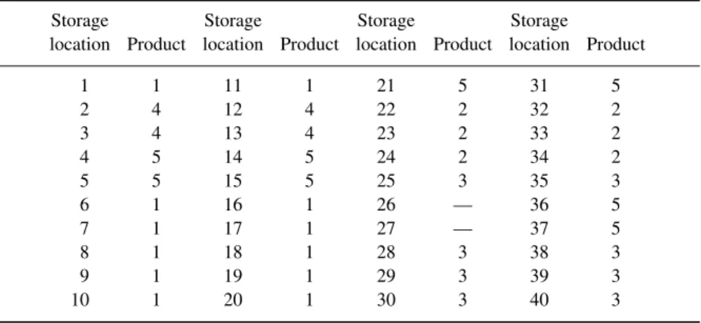
Malabar Ltd is an Indian company having a warehouse with two I/O ports and 40 storage locations, arranged in four racks (see Figure 5.17). The characteristics of the products at stock are reported in Table 5.5, while the distances between the two I/O ports and the storage locations are indicated in Tables 5.6 and 5.7. The optimal product allocation can found through model (5.16)–(5.18), (5.20), in whichn =5,
md=40, whilemj, j =1, . . . ,5 are calculated on the basis of the second column
of Table 5.5. Cost coefficientscj k, j = 1, . . . ,5, k =1, . . . ,40, are indicated in
Tables 5.8 and 5.9 and calculated using Equation (5.15), where it is assumed that travel time trk from I/O port r = 1,2, to storage locationk, k = 1, . . . ,40, is
Table 5.9 Cost coefficientscj k, j=1, . . .5, k=21, . . . ,40, in the Malabar problem.
Assignment cost
Storage Product Product Product Product Product
locationk j=1 j=2 j=3 j=4 j=5
21 44.17 80.67 62.00 139.00 66.00
22 45.33 77.33 58.00 140.00 66.00
23 46.50 74.00 54.00 141.00 66.00
24 47.67 70.67 50.00 142.00 66.00
25 48.83 67.33 46.00 143.00 66.00
26 47.75 87.67 67.50 150.50 71.50
27 48.92 84.33 63.50 151.50 71.50
28 50.08 81.00 59.50 152.50 71.50
29 51.25 77.67 55.50 153.50 71.50
30 52.42 74.33 51.50 154.50 71.50
31 44.17 80.67 62.00 139.00 66.00
32 45.33 77.33 58.00 140.00 66.00
33 46.50 74.00 54.00 141.00 66.00
34 47.67 70.67 50.00 142.00 66.00
35 48.83 67.33 46.00 143.00 66.00
36 47.75 87.67 67.50 150.50 71.50
37 48.92 84.33 63.50 151.50 71.50
38 50.08 81.00 59.50 152.50 71.50
39 51.25 77.67 55.50 153.50 71.50
40 52.42 74.33 51.50 154.50 71.50
Table 5.10 Optimal allocation of products in the Malabar warehouse.
Storage Storage Storage Storage
location Product location Product location Product location Product
1 1 11 1 21 5 31 5
2 4 12 4 22 2 32 2
3 4 13 4 23 2 33 2
4 5 14 5 24 2 34 2
5 5 15 5 25 3 35 3
6 1 16 1 26 — 36 5
7 1 17 1 27 — 37 5
8 1 18 1 28 3 38 3
9 1 19 1 29 3 39 3
If the warehouse has a single I/O port (R = 1), the problem solving method-ology can be simplified. In fact, under this hypothesis, cost coefficientscj k, j =
1, . . . , n, k=1, . . . , md, take the following form,
cj k=
pj1
mj
t1k =ajbk,
whereaj =pj1/mj andbk =t1kdepend only on productj and on storage location
k, respectively. Then, the optimal product allocation can be determined by using the following procedure.
Step 1. Construct a vectorαofnj=1mjcomponents, in which there aremjcopies of
eachaj, j =1, . . . , n. Sort the vectorαby nonincreasing values of its components.
Defineσα(i)in such a way thatσα(i)=j ifαi =aj, i=1, . . . ,nr=1mr.
Step 2. Letb be the vector of md components corresponding to values bk, k =
1, . . . , md. Sort the vectorbby nondecreasing values of its components. Letβbe the
vector ofnj=1mj components, corresponding to the first
n
j=1mj components
of the sorted vectorb. Defineσβ(i)in such a way thatσβ(i)=kifβi =bk, i=
1, . . . ,nr=1mr.
Step 3. Determine the optimal solution of problem (5.16)–(5.18), (5.20) as
xσ∗α(i),σβ(i)=1, i=1, . . . ,
n
j=1
mj
andxj k∗ =0, for all the remaining components.
This procedure is based on the fact that the minimization of the scalar product of two vectorsα andβ is achieved by ordering αby nonincreasing values andβ by nondecreasing values.
If the warehouse of Malabar company (see the previous problem) has a single I/O port (corresponding to port 1 in Figure 5.17), the coefficientsaj, j =1, . . . ,5, are
those reported in Table 5.11. For the sake of simplicity, travel times are assumed to be equal to distances (see Table 5.6). Values ofαi,σα(i),βi,σβ(i), i =1, . . . ,38,
are reported in Table 5.12. The optimal solution is reported in Table 5.13. It is worth noting that no item is allocated to the storage locations farthest from the I/O port (locations 30 and 40).
5.4
Operational Decisions
Table 5.11 Characteristics of products in the Malabar problem.
Product Storage Number of storages and
(j) locations retrievals per day aj
1 12 43 3.58
2 6 42 7.00
3 8 44 5.50
4 4 46 11.50
5 8 44 5.50
Table 5.12 Values ofαi,σα(i),βi,σβ(i), fori=1, . . . ,38, in the Malabar problem.
i αi σα(i) βi σβ(i) i αi σα(i) βi σβ(i)
1 11.50 4 2 1 20 5.50 5 11 20
2 11.50 4 2 11 21 5.50 5 14 21
3 11.50 4 3 6 22 5.50 5 14 31
4 11.50 4 3 16 23 5.50 5 15 26
5 7.00 2 4 2 24 5.50 5 15 36
6 7.00 2 4 12 25 5.50 5 16 22
7 7.00 2 5 7 26 5.50 5 16 32
8 7.00 2 5 17 27 3.58 1 17 27
9 7.00 2 6 3 28 3.58 1 17 37
10 7.00 2 6 13 29 3.58 1 18 23
11 5.50 3 7 8 30 3.58 1 18 33
12 5.50 3 7 18 31 3.58 1 19 28
13 5.50 3 8 4 32 3.58 1 19 38
14 5.50 3 8 14 33 3.58 1 20 24
15 5.50 3 9 9 34 3.58 1 20 34
16 5.50 3 9 19 35 3.58 1 21 29
17 5.50 3 10 5 36 3.58 1 21 39
18 5.50 3 10 15 37 3.58 1 22 25
19 5.50 5 11 10 38 3.58 1 22 35
technologies and policies are used: the formation of batches (see Section 5.4.1), picker routing (see Section 5.4.2), S/R machine scheduling (see Problem 5.4) and vehicle loading (see Section 5.4.3).
5.4.1
Batch formation
Table 5.13 Optimal product allocation to storage locations in the Malabar problem.
Storage Storage Storage Storage
location Product location Product location Product location Product
1 4 11 4 21 5 31 5
2 2 12 2 22 5 32 5
3 2 13 2 23 1 33 1
4 3 14 3 24 1 34 1
5 3 15 3 25 1 35 1
6 4 16 4 26 5 36 5
7 2 17 2 27 1 37 1
8 3 18 3 28 1 38 1
9 3 19 3 29 1 39 1
10 5 20 5 30 — 40 —
In the first stage, the optimal batch sized∗is estimated in an attempt to balance the picking and sorting efforts. Then in Step 2 batches are created according to a ‘first come first served’ (FCFS) policy by aggregatingd∗consecutive orders.
Batch sizing. Batches are sized in an attempt to minimize the total workload, which is the sum of the total picking and sorting times. In what follows, this approach is illustrated for the configuration in Figure 5.18, in which goods are retrieved by one or more pickers and then transported to the shipping zone by a belt conveyor.
Leto be the average number of orders per time period,uthe average number of items in an order,t1the time needed to make a path including all storage locations,
t2the traversal time on foot of the shipping zone, where orders are assembled. The
decision variable is the average number of orders in a lotd.
Under the hypothesis that the items are uniformly distributed and that each batch is made up of many items, the time spent for picking a batch is approximatelyt1. As
o/d is the average number of pickings per time period, the time devoted to picking operations isot1/dper time period. On the other hand, the time spent for sorting the
items in the shipping zone isαuot2d, whereα∈ (0,1)is a parameter to be defined
either empirically or through a simulation model. In order to determine the optimal
dvalue, the following model has to be solved.
Minimize
ot1
d +αuot2d (5.21)
subject to
d 0, integer, (5.22)
Shipping zone
Figure 5.18 Batch picking in a warehouse equipped with a belt conveyor.
Step 1. Determine the minimum pointd of functionc(d) = ot1/d+αuot2d, by
imposing that the first derivative ofc(d)becomes zero:
d=
t1
αut2
.
Step 2. Letd∗= difc(d) < c(d), otherwised∗= d.
Hence,d∗increases as the size of the storage zone increases, and decreases as the average number of items in an order increases.
Clavier distributes French ties in Brazil. Its warehouse located in Manaus has a layout similar to the one represented in Figure 5.18, with 15 aisles, each one of which is 25 m long and 3.5 m wide. The area occupied by a pallet is 1.05×1.05 m2. The vehicles used for picking goods move at about 3.8 km/h, while the time to traverse the shipping zone on foot is about 1.5 min. The average number of orders handled in a day is 300, and the average number of items in an order is 10. The parameterαhas been empirically set equal to 0.1. Hence,
t1=
1.05+25×30+3.5×15+1.05×28
3800 ×60=13.15 min.
and
d=
13.15
Figure 5.19 Routing of a picker in a storage zone with side aisles having a single entrance (the dark-coloured storage locations are the ones where a retrieval has to be performed).
5.4.2
Order picker routing
In W/RPSs, where pickers travel on foot or by motorized trolley and may visit multi-ple aisles, order picker routing is a major issue. Picker routing is part of a large class of combinatorial optimization problems known asvehicle routing problems(VRPs), which will be examined extensively in Chapter 7 in the context of distribution man-agement. In this section a single picker problem, known asroad travelling salesman problem(RTSP), is illustrated. The RTSP is a slight variant of the classicaltravelling salesman problem(TSP) (see Section 7.3) and consists of determining a least-cost tour including a subset of vertices of a graph. The RTSP is NP-hard, but, in the case of warehouses, it is often solvable in polynomial time due to the particular charac-teristics of the travel network. If each aisle has a single entrance, the least duration route is obtained by first visiting all the required storage locations placed in the upper side aisles and then the required storage locations situated in the lower side aisles (see Figure 5.19). On the other hand, if the side aisles have some interruptions (i.e. if there is more than one cross aisle), the problem can be solved to optimality by using the Ratliff and Rosenthal dynamic programming algorithm, whose worst-case computational complexity is a linear function of the number of side aisles. However, if there are several cross aisles, the number of states and transitions increases rapidly and the use of the dynamic programming procedure becomes impractical. Therefore, in what follows, two simple heuristics are illustrated. The reader interested in the Ratliff and Rosenthal algorithm is referred to the list at the end of the chapter.
Figure 5.20 Routing of a picker in a storage zone with side aisles having two entrances (the dark-coloured storage locations are the ones where a retrieval has to be performed).
Largest gap heuristic. In this context, agapis the distance between any two adja-cent items to be retrieved in an aisle, or the distance between the last item to be retrieved in an aisle and the closest cross aisle. The picker goes to the front of the side aisle, closest to the I/O port, including at least one item to be retrieved. Then the picker traverses the aisle entirely, while the remaining side aisles are entered and left once or twice, both times from the same side, depending on the largest gap of the aisle.
Golden Fruit is an Honduran company manufacturing fruit juice. Last 17 Septem-ber, a picker routing problem had to be solved at 10:30 a.m. in the warehouse located in Puerto Lempira (see Figure 5.20). Travel times were assumed to be proportional to distances. The routes provided by the S-shape and largest gap heuristics are shown in Figures 5.21 and 5.22, respectively, and the least-cost route is illustrated in Fig-ure 5.23.
5.4.3
Packing problems
Figure 5.21 Picker route provided by the S-shape heuristic in the Golden Fruit warehouse.
Figure 5.22 Picker route provided by the largest gap heuristic in the Golden Fruit warehouse.
of required bins. Constraints on the stability of the load are sometimes imposed. From a mathematical point of view, packing problems are mostly NP-hard, so that in most decision support systems heuristics are used.
Classification. In some packing problems, not all physical characteristics of the items have to be considered when packing. For instance, when loading high-density goods onto a truck, items can be characterized just by their weight, without any concern for their length, width and height. As a result, packing problems can be classified according to the number of parameters needed to characterize an item.
Figure 5.23 Least cost picker route in the Golden Fruit warehouse.
• Two-dimensional packing problemsusually arise when loading a pallet with items having the same height.
• Three-dimensional packing problems occur when dealing with low-density items, in which case volume is binding.
In the following, it is assumed, for the sake of simplicity, that items are rectangles in two-dimensional problems, and that their sides must be parallel or perpendicular to the sides of the bins in which they are loaded. Similarly, in three-dimensional problems, the items are assumed to be parallelepipeds and their surfaces are parallel or perpendicular to the surfaces of the bins in which they are loaded. These assumptions are satisfied in most settings.
Packing problems are usually classified asoff-lineandon-lineproblems, depending on whether the items to be loaded are all available or not when packing starts. In the first case, item characteristicscanbe preprocessed (e.g. items can be sorted by nondecreasing weights) in order to improve heuristic performance. A heuristic using such preprocessing is said to beoff-line, otherwise it is calledon-line. Clearly, an on-line heuristic can be used for solving an off-line problem, but an off-line heuristic cannot be used for solving an on-line problem.
One-dimensional packing problems
The simplest one-dimensional packing problem is known asbin packing(1-BP) prob-lem. It amounts to determining the least number of identical capacitated bins in which a given set of weighted items can be accommodated. Letmbe the number of items to be loaded;nthe number of available bins (or an upper bound on the number of bins in an optimal solution);pi, i=1, . . . , m, the weight of itemi;qj the capacity
of binj, j =1, . . . , n. The problem can be modelled by means of binary variables
j or 0 otherwise, and binary variablesyj, j =1, . . . , n, equal to 1 if binj is used, 0
otherwise. The 1-BP problem can then be modelled as follows.
Minimize
n
j=1
yj (5.23)
subject to
n
j=1
xij =1, i=1, . . . , m, (5.24) m
i=1
pixij qyj, j =1, . . . , n, (5.25)
xij ∈ {0,1}, i=1, . . . , m, j=1, . . . , n,
yj ∈ {0,1}, j =1, . . . , n.
The objective function (5.23) is the number of bins used. Constraints (5.24) state that each item is allocated to exactly one bin. Constraints (5.25) guarantee that bin capacities are not exceeded.
A lower boundz(I )on the number of bins in any 1-BP feasible solution can be easily obtained as
z(I )= (p1+p2+ · · · +pm)/q. (5.26)
The lower bound (5.26) can be very poor if the average number of items per bin is low (see Problem 5.8 for an improved lower bound). Such lower bounds can be used in a branch-and-bound framework or to evaluate the performance of heuristic methods. In the remainder of this section, four heuristics are illustrated. The first two procedures (thefirst fit (FF) and thebest fit (BF) algorithms) are on-line heuristics while the others are off-line heuristics.
FF algorithm.
Step 0. LetSbe the list of items,V the list of available bins andT the list of bins already used. Initially,T is empty.
Step 1. Extract an itemifrom the top of listSand insert it into the first binj ∈T
having a residual capacity greater than or equal topi. If no such bin exists, extract
from the top of listV a new binkand put it at the bottom ofT; insert itemiinto bink.
BF algorithm.
Step 0. LetSbe the list of items to be packed,V the list of available bins andT the list of bins already used. Initially,T is empty.
Step 1. Extract an itemifrom the top of listSand insert it into the binj ∈T whose residual capacity is greater than or equal topi, and closer topi. If no such bin
exists, extract a new binkfrom the top ofV and put it at the bottom ofT; insert itemiinto bink.
Step 2. IfS= ∅,STOP, all the items have been loaded,T represents the list of the bins used, whileV is the list of bins unused. IfS= ∅, go back to step 1.
The two procedures can both be implemented so that the computational complexity is equal toO(mlogm).
It is useful to characterize the performance ratios of such heuristics. Recall that the performance ratioRHof a heuristic H is defined as
RH=sup
I
zH(I ) z∗(I )
,
whereIis a generic instance of the problem,zH(I )is objective function value of the solution provided by heuristic H for instanceI, whilez∗(I )represents the optimal solution value for the same instance.
This means that
• zH(I )/z∗(I )RH, ∀I;
• there are some instancesIsuch thatzH/z∗(I )is arbitrarily close toRH.
Unfortunately, the worst-case performance ratios of the FF and BF heuristics are not known, but it has been proved that
RFF74 and RBF 74.
The FF and BF algorithms can be easily transformed into off-line heuristics, by preliminary sorting the items by nonincreasing weights, yielding thefirst fit decreasing (FFD) and thebest fit decreasing(BFD) algorithms. Their complexity is still equal to
O(mlogm), while their performance ratios are
RFFD=RFBFD= 32.
It can be proved that this is the minimum worst-case performance ratio that a polynomial 1-BP heuristic can have.
Table 5.14 Weight of the parcels (in kilograms) in the Al Bahar problem.
Number of parcels Weight
4 252
3 228
3 180
3 140
4 120
Table 5.15 Sorted list of the parcels in the Al Bahar problem (parcel weights are expressed in kilograms).
Parcel Weight Parcel Weight
1 252 10 180
2 252 11 140
3 252 12 140
4 252 13 140
5 228 14 120
6 228 15 120
7 228 16 120
8 180 17 120
9 180
BFD heuristic, the parcels are sorted by nonincreasing weights (see Table 5.15) and the solution reported in Table 5.16 is obtained. The number of trips is six. The lower bound on the number of trips given by Equation (5.26) is3132/600 = 6. Hence, the BFD heuristic solution is optimal.
Two-dimensional packing problems
The simplest two-dimensional packing problem (referred to as the 2-BP problem in the following) consists of determining the least number of identical rectangular bins in which a given set of rectangular items can be accommodated. It is also assumed that no item rotation is allowed. LetLandW be the length and the width of a bin, respectively, and letli andwi, i=1, . . . , m, be the length and the width of itemi.
A lower boundz(I )on the number of bins in any feasible solution is
z(I )= (l1w1+l2w2+ · · · +lmwm)/LW.
Table 5.16 Parcel-to-trip allocation in the optimal solution of the Al Bahar problem (parcel weights are expressed in kilograms).
Parcel Weight Trip Parcel Weight Trip
1 252 1 10 180 5
2 252 1 11 140 3
3 252 2 12 140 5
4 252 2 13 140 5
5 228 3 14 120 5
6 228 3 15 120 6
7 228 4 16 120 6
8 180 4 17 120 6
9 180 4
Layer 2
W
L
Layer 1
Figure 5.24 Layers of items inside a bin.
longest item. All the items of a layer are located on its bottom, which corresponds to the level of the longest item of the previous layer (see Figure 5.24).
Here we illustrate two off-line heuristics, namedfinite first fit(FFF) andfinite best fit(FBF) heuristics.
FFF algorithm.
Step 0. LetSbe the list of items, sorted by nonincreasing lengths,V the list of bins andT the list of bins used. Initially,T is empty.
can accommodate the layer, extract from the top ofV a new binkand put it at the bottom ofT, load itemiinto the leftmost position at the bottom of bink.
Step 2. IfS= ∅,STOP, all the item have been loaded. Then,T represents the list of bins used, whileV provides the list of the unused bins. IfS= ∅, go back to step 1.
FBF algorithm.
Step 0. LetSbe the list of items, sorted by nonincreasing lengths,V the list of bins andT the list of bins used. Initially,T is empty.
Step 1. Extract an itemifrom the top of Sand insert it into the leftmost position of the layer of a binj ∈T whose residual width is greater than or equal to, and closer to, item width. If no such layer exists, create a new one in the bin ofT whose residual length is greater than or equal to, and closer to, the length of itemi. Then, introduce itemiin the leftmost position of the layer. If there is no bin ofT which can accommodate the layer, extract from the top ofV a new binkand put it at the bottom ofT, load itemiinto the leftmost position at the bottom of bink.
Step 2. IfS= ∅,STOP, all the item have been loaded. Then,T represents the list of bins used, whileV provides the list of the unused bins. IfS = ∅, go back to step 1.
Such layer heuristics have a low computational complexity, since the effort for selecting the layer where an item has to be inserted is quite small. However, they can turn out to be inefficient if the average number of items per bin is relatively small. In such a case, the followingbottom left(BL) algorithm usually provides better solutions.
BL algorithm.
Step 0. LetSbe the list of items, sorted by nonincreasing lengths,V the list of bins andT the list of bins used. Initially,T is empty.
Step 1. Extract an itemifrom the top of listSand insert it into the leftmost position at the bottom of the first binj ∈T able to accommodate it. If no such bin exists, extract a new binkfrom the top ofV, and put it at the bottom ofT; load itemi
into the leftmost position at the bottom of bink.
Step 2. IfS= ∅,STOP, all the items have been loaded,T represents the list of bins used, whileV provides the list of bins unused. IfS= ∅, go back to step 1.
Table 5.17 Characteristics of ISO 40 container.
Length Width Height Capacity Capacity
(m) (m) (m) (m3) (kg)
12.069 2.373 2.405 68.800 26.630
Table 5.18 Parcels shipped by Kumi company.
Length Width Height
Quantity (m) (m) (m)
6 1.50 1.50 2.00
5 1.20 1.70 2.00
13 1.00 1.00 1.00
11 0.80 0.50 1.00
L
2
W
2
2 2
2 2
2
2 2
2
L
W
2 2
Figure 5.25 Parcels allocated to the two containers shipped by Kumi company (2 indicates two overlapped parcels).
pairs of (0.8×0.5) m2parcels. Then, each such a pair is considered as a single item.
Applying the FBF algorithm, the solution reported in Figure 5.25 is obtained.
Three-dimensional packing problems
Table 5.19 Parcels loaded at McMillan company.
Length Width Height Volume Weight
Type Quantity (m) (m) (m) (m3) (kg)
1 2 2.50 0.75 1.30 2.4375 75.00
2 4 2.10 1.00 0.95 1.9950 68.00
3 7 2.00 0.65 1.40 1.8200 65.50
4 4 2.70 0.70 0.95 1.7900 63.00
5 3 1.40 1.50 0.80 1.6800 61.50
bins in which a given set of parallelepipedic items can be accommodated. It is also assumed that no item rotation is allowed. LetL,W andHbe the length, width and height of a bin, respectively, and letli,wiandhi, i =1, . . . , m, be the length, width
and height of itemi.
A lower boundz(I )on the number of bins is
z(I )= l1w1h1+l2w2h2+ · · · +lmwmhm)/LW H. (5.27)
The simplest heuristics for 3-BP problems insert items sequentially into layers parallel to some bin surfaces (e.g. toW×H surfaces). In the following a heuristics based on this principle is illustrated.
3-BP-L algorithm.
Step 0. LetSbe the list of items.
Step 1. Solve the 2-BP problem associated withmitems characterized bywi,hi, i=
1, . . . , m, and bins characterized byWandH. Letkbe the number of bidimensional bins used (referred to assectionsin the following). The length of each section is equal to the length of the largest item loaded into it.
Step 2. Solve the 1-BP problem associated with theksections, each of which has a weight equal to its length, while bins have a capacity equal toL.
If the items are all available when bin loading starts, it can be useful to sort listS
by nonincreasing values of the volume. However, unlike one-dimensional problems, more complex procedures are usually needed to improve solution quality.
Table 5.20 Characteristics of the vehicles in the McMillan problem.
Length Width Height Capacity Capacity
(m) (m) (m) (m3) (kg)
6.50 2.40 1.80 28.08 12.30
5 5
W
H
2 3 3 4
W
H
2 2
3 4
W
1 1
2 4
W
3
3 5
W
3 3
4
W
Figure 5.26 Sections generated at the end of Step 1 of the 3-BP-L heuristic in the McMillan problem.
cannot be rotated. First, the parcels are sorted by nonincreasing volumes. Then, the 3-BP-L algorithm (in which 2-BP problems are solved through the BL heuristic) is used. The solution is made up of six (2.4×1.8) m2sections, loaded as reported in Figure 5.26. Finally, a 1-BP problem is solved by means of the BFD heuristic. In the solution (see Table 5.22) three vehicles are used, the most loaded of which carries a weight of 545.5 kg, much less than the weight capacity. It is worth noting that the lower bound provided by Equation (5.27) is37.795/28.08 =2.
5.5
Questions and Problems
5.1 Show that a warehouse can be modelled as a queueing system.
5.2 A warehouse stores nearly 20 000 pallets. Goods turn about five times a year. How much is the required labour force? Assume two eight-hour shifts per day and about 250 working days per year. (Hint: apply Little’s Law stating that for a queueing system in steady state the average lengthLQof the queue equals
Table 5.21 Width of the sections generated at the end of Step 1 of the 3-BP-L heuristic in the McMillan problem.
Width Weight
Section (m) (kg)
1 2.70 281.00
2 2.70 264.50
3 2.70 262.00
4 2.70 194.00
5 2.00 192.50
6 1.40 123.00
Table 5.22 Section allocation to vehicles at the end of Step 2 of the 3-BP-L heuristic in the McMillan problem.
Section Vehicle
1 1
2 1
3 2
4 2
5 3
5.3 Letdbe the daily demand from all orders,lCthe average length of a rail car,q
the capacity of a rail car andnCthe number of car changes per day. Estimate
the length of rail docklDneeded by a warehouse.
5.4 Show that scheduling an S/R machine can be modelled as a rural postman problem on a directed graph. The rural postman problem consists of determining a least-cost route traversing a subset of required arcs of a graph at least once (see Section 7.6.2 for further details).
5.5 Show that an optimal picker route cannot traverse an aisle (or a portion of an aisle) more than twice. Illustrate how this property can be used to devise a dynamic programming algorithm.
5.6 Demonstrate that both the FF and BF heuristics for the 1-BP problem take
O(mlogm)steps.
5.7 Devise a branch-and-bound algorithm based on formula (5.26).
5.8 Devise an improved 1-BP lower bound.
5.9 Modify the heuristics for the 1-BP problem for the case where each binj, j =
1, . . . , n, has a capacityqj and a costfj. Apply the modified version of the
Table 5.23 List of the parcels to load and corresponding weight (in kilograms) in the Brocard problem.
Parcel Weight Parcel Weight
1 228 18 170
2 228 19 170
3 228 20 170
4 217 21 170
5 217 22 95
6 217 23 95
7 217 24 95
8 210 25 95
9 210 26 75
10 210 27 75
11 210 28 75
12 195 29 75
13 195 30 75
14 195 31 75
15 170 32 55
16 170 33 55
17 170 34 55
mainly in France and in the Benelux. The vehicle fleet comprises 14 vans of capacity equal to 800 kg and 22 vans of capacity equal to 500 kg. The company has to deliver on behalf of the EU 34 parcels of different sizes from Paris to Frankfurt (the distance between these cities is 592 km). The characteristics of the parcels are reported in Table 5.13. As only five company-owned vans (all having capacity of 800 kg) will be available on the day of the delivery, Brocard has decided to hire additional vehicles from a third-party company. The following additional vehicles will be available:
• two trucks with a capacity of 3 tons each, whose hiring total cost (inclusive of drivers) is€1.4 per kilometre;
• one truck with trailer, with a capacity of 3.5 tons, whose hiring total cost (inclusive of drivers) is€1.6 per kilometre.
Which trucks should Brocard hire?
5.6
Annotated Bibliography
A recent survey on warehouse design and control is:
1. Jeroen P and Van den Berg L 1999 A literature survey on planning and control of warehousing systems.IIE Transactions31, 751–762.
An in-depth treatment of warehouse management is:
2. Bartholdi JJ and Hackman ST 2002Warehouse and Distribution Science. (Available at http://www.warehouse-science.com.)
A dynamic programming algorithm for the picker routing problem in Section 5.4.2 is presented in:
3. Ratliff HD and Rosenthal AS 1983 Order picking in a rectangular warehouse: a solvable case of the travelling salesman problem.Operations Research31, 507–521.
A survey of packing problems is:
4. Dowsland KA and Dowsland WB 1992 Packing problems.European Journal of Operational Research56, 2–14.
An annotated bibliography on packing problems is:
5. Dyckhoff H, Scheithauer G and Terno J 1997 Cutting and packing. InAnnotated Bibliographies in Combinatorial Optimization(ed. Dell’Amico M, Maffioli F and Martello S). Wiley, Chichester.
For a detailed treatment of 1-BP, Chapter 8 of the following book is recommended:
6. Martello S and Toth P 1990Knapsack Problems: Algorithms and Computer Implementations. Wiley, Chichester.
Two recent papers on exact algorithms for two and three-dimensional packing prob-lems are:
7. Martello S and Vigo D 1998 Exact solution of the two-dimensional finite bin packing problem.Management Science44, 388–399.