GENERATION TRIPPING FOR TRANSIENT STABILITY CONTROL USING THE EMERGENCY SINGLE MACHINE EQUIVALENT METHOD

R

REEQQUUIIRREEMMEENNTT FFOORR TTHHEE DEDEGGRREEEE OOFF:: M

MAASSTTEERR OFOF SSCCIIENENCCEESS I

INN ELELEECCTTRRIICCAALL EENNGGIINNEEEERRIINNGG

BBYY

LAURA LETICIA JUÁREZ CALTZONTZIN

M

MÉÉXXIICOCO,, DD.. F.F. 22001100

GENERATION TRIPPING FOR TRANSIENT

STABILITY CONTROL USING THE EMERGENCY

SINGLE MACHINE EQUIVALENT METHOD

E

E

S

S

C

C

U

U

E

E

L

L

A

A

S

S

U

U

P

P

E

E

R

R

I

I

O

O

R

R

D

D

E

E

I

I

N

N

G

G

E

E

N

N

I

I

E

E

R

R

Í

Í

A

A

M

M

E

E

C

C

Á

Á

N

N

I

I

C

C

A

A

Y

Y

E

E

L

L

É

É

C

C

T

T

R

R

I

I

C

C

A

A

S

S

E

E

C

C

C

C

I

I

Ó

Ó

N

N

D

D

E

E

E

E

S

S

T

T

U

U

D

D

I

I

O

O

S

S

D

D

E

E

P

P

O

O

S

S

G

G

R

R

A

A

D

D

O

O

E

E

I

I

N

N

V

V

E

E

S

S

T

T

I

I

G

G

A

A

C

C

I

I

Ó

Ó

N

N

D

A

BSTRACT

System Protection Schemes (SPS) like generation tripping, load shedding and other stability controls apply emergency control actions in order to stabilize the electric power system when a severe contingency, causing a large unbalance between generation and load powers, occurs.

Most practical generation tripping schemes for controlling transient stability problems, commonly used these days, are based on the occurrence of a specific event and are designed and adjusted by means of off-line studies; however, inaccuracies in the system dynamic model and unpredicted operating conditions that may appear in actual system operation, could make the SPS fail. In order to avoid these problems, measurement-based SPS have been proposed, which use real-time measurements in order to assess the severity of the problem and to adapt the size and location of the control action needed to stabilize the system when an actual contingency occurs.

This work describes the emergency single machine equivalent method (E-SIME for short), which has been developed for controlling transient stability problems using real-time measurements. The following aspects of E-SIME are developed and described in detail:

• Basics of the SIngle Machine Equivalent (SIME) method.

• The main steps of the Emergency SIME method:

-Predictive transient stability assessment using power and rotor angle measurements.

-Determination of the size and location of the control action to stabilize the system.

• Structure and development of a new computer program able to apply the method.

• Application and performance testing of E-SIME in systems having different structures, sizes and operating conditions.

• Discussion of the method practical implementation issues and cases where the method needs improvements.

R

ESUMEN

Los esquemas de protección a nivel del sistema como el disparo de generación, el tiro de carga y otros controles de estabilidad aplican acciones de control de emergencia para estabilizar al sistema eléctrico de potencia cuando una contingencia severa, que causa un gran desbalance entre las potencias de generación y carga, ocurre.

La gran mayoría de los esquemas prácticos de disparo de generación para controlar problemas de estabilidad transitoria, utilizados comúnmente estos días, están basados en la ocurrencia de un evento específico y son diseñados y ajustados por medio de estudios realizados fuera de línea; sin embargo, inexactitudes en el modelo dinámico del sistema y condiciones de operación imprevistas que pueden aparecer en la operación real del sistema de potencia, pueden hacer que falle el esquema de protección a nivel del sistema. Para evitar estos problemas, se han propuesto esquemas de protección a nivel del sistema basados en mediciones, lo cuales utilizan mediciones en tiempo real para evaluar la severidad del problema y para adaptar la magnitud y la localización de la acción de control necesaria para estabilizar el sistema de potencia cuando ocurre una contingencia.

Este trabajo describe el método de emergencia de la máquina equivalente, que ha sido desarrollado para controlar problemas de estabilidad transitoria utilizando mediciones en tiempo real. Los siguientes aspectos de este método son desarrollados y descritos en detalle:

• Los conceptos básicos del método de la máquina equivalente.

• Los dos pasos principales del método de emergencia de la máquina equivalente:

-Evaluación predictiva de la estabilidad transitoria utilizando mediciones de potencias y ángulos de carga.

-Determinación de la magnitud y localización de la acción de control para estabilizar al sistema.

• La estructura y el desarrollo de un nuevo programa de computadora que aplica el método.

• La aplicación y prueba del desempeño del método en sistemas con diferentes estructuras, tamaños y condiciones de operación.

• La discusión de los aspectos de implementación práctica del método y casos en los que el método necesita ser mejorado.

D

EDICATORIA

Dedicado a la memoria de Antonio Munguía y González Castillo, su recuerdo siempre será inspiración para todos los que tuvimos la fortuna de conocerlo.

A mis familiares, por su apoyo incondicional, especialmente por comprender estos años de continuas ausencias y motivarme en todo momento.

A mis queridos amigos por mantenerme en sus pensamientos y ofrecerme en todo momento su amistad e invaluables consejos, en especial a Rubén, Pamela, Hitoshi, Rodrigo, Gus y José Luis.

A mis amados hermanos Gustavo, Marisol y Arturo, ¿que les puedo decir?, ¿Felicidades?...no hay palabras para expresar lo que significan para mi.

A mis padres, las personas a quien más amo y admiro, su ejemplo de superación será siempre un incentivo para lograr todos mis objetivos.

A

CKNOWLEDGEMENTS

I would like to express my sincere gratitude to Dr. Daniel Ruiz Vega for the direction of this work and to the members of the jury: Drs. Daniel Olguín Salinas, David Romero Romero, Ricardo Mota Palomino, Germán Rosas Ortiz and Tomás Ignacio Asiaín Olivares. Their valuable advices and recommendations were always oriented to improve the present work.

I would like to express my warmest thanks to M.S. Arturo Galán Martinez and Dr. Jaime Robles García for the personal interest they have had in my work.

The validation of the generation tripping could not have been possible without the data files provided by M.S. David Villareal Martínez and the kind help of Miguel Alvarez Juárez.

A special acknowledgement to the amazing guys I met during this research work: Gustavo Trinidad Hernández, José Luis Valenzuela Salazar, Miguel Alvarez Juárez, Jesús Carmona Sánchez and Héctor Manuel Sánchez García, for their continuous support, encouragement and friendship.

The financial support of CONACyT and IPN is also gratefully acknowledged for the MSc. scholarship, the thesis scholarship and the PIFI scholarship in projects SIP 20090918 and 20100895.

C

ONTENTS

Page

ABSTRACT ... VII RESUMEN ...IX DEDICATORIA ...XI ACKNOWLEDGEMENTS ...XIII CONTENTS ... XV LIST OF FIGURES... XVII LIST OF TABLES...XXI GLOSSARY ...XXIII NOMENCLATURE ... XXV

CHAPTER 1: INTRODUCTION ... 1

1.1INTRODUCTION... 1

1.2OBJECTIVE OF THE THESIS... 2

1.3HISTORICAL BACKGROUND AND MOTIVATION... 3

1.3.1 The SIME method... 3

1.3.2 The E-SIME method ... 5

1.4JUSTIFICATION... 6

1.5SCOPE... 7

1.6CONTRIBUTIONS... 7

1.7PUBLICATIONS DERIVED FROM THE THESIS... 8

1.8THESIS ORGANIZATION... 8

CHAPTER 2: TRANSIENT STABILITY CONTROL ... 9

2.1INTRODUCTION... 9

2.2POWER SYSTEM STABILITY... 11

2.2.1 Power system stability classification ... 13

2.2.2 Power system instability classification ... 15

2.3TRANSIENT STABILITY... 16

2.3.1 Transient stability approaches... 19

2.3.2 Transient stability assessment using the EAC... 22

2.4CONTROL OF TRANSIENT STABILITY... 24

2.4.1 Preventive control of transient stability problems ... 28

2.4.2 Emergency control of transient stability problems ... 29

2.4.3 Preventive vs Emergency control... 38

2.4.2 On-line and real time control of transient stability... 40

CHAPTER 3: THE EMERGENCY SIME METHOD ... 43

3.1INTRODUCTION... 43

3.2THE SIME METHOD... 43

3.2.1 Foundations of the SIME method... 44

3.2.2 Overall formulation of the SIME method... 45

Page

3.2.4 Stability margins... 48

3.3THE EMERGENCY SIME METHOD... 49

3.3.1 Principle ... 50

3.3.2 Description of the predictive assessment method ... 52

3.3.3 Description of the emergency control design method... 55

3.4PRACTICAL CONSIDERATIONS FOR THE APLICATION OF THE E-SIME METHOD... 62

3.5REAL TIME MEASUREMENTS CURRENTLY AVAILABLE... 63

3.6DIGITAL COMPUTER PROGRAM... 65

3.7COUPLING THE TIME DOMAIN SIMULATION COMPUTER PROGRAM WITH THE E-SIME METHOD COMPUTER PROGRAM... 69

CHAPTER 4: APPLICATION OF THE METHODOLOGY AND ANALYSIS OF RESULTS ... 71

4.1INTRODUCTION... 71

4.2 THE IEEE THREE-MACHINE TEST POWER SYSTEM... 71

4.3NEW ENGLAND TEST SYSTEM... 83

4.4PROPOSED SOUTH-EASTERN EQUIVALENT MEXICAN TEST SYSTEM SIEQ ... 90

CHAPTER 5: CONCLUSIONS... 97

5.1CONCLUSIONS... 97

5.1.1 Real-time measurements... 97

5.1.2 Stability prediction ... 98

5.1.3 Corrective actions ... 99

5.1.4 Behavior of the method... 99

5.2FUTURE WORKS... 101

REFERENCES... 103

APPENDIX A TEST SYSTEMS DATA ... 109

A.1EQUIVALENT MMT TEST SYSTEM... 109

A.2THREE-MACHINE TEST SYSTEM... 110

A.3NEW ENGLAND TEST SYSTEM... 112

A.4PROPOSED SOUTH-EASTERN EQUIVALENT MEXICAN TEST SYSTEM SIEQ ... 115

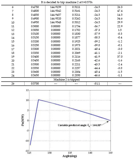
APPENDIX B: GENERATION TRIPPING VALIDATION... 121

L

IST OF

F

IGURES

Page

FIGURE 2.1SIGNIFICANT EVENTS IN THE EVOLUTION OF POWER SYSTEM CONTROL TECHNOLOGY [RUIZ-VEGA,2009].ADAPTED FROM [HANDSCHIN AND PETROIANU,1991] AND UPDATED

FROM [RUIZ-VEGA,2002A]. ... 10

FIGURE 2.2MEASURED VALUES OF THE MEXICAN NATIONAL INTERCONNECTED POWER SYSTEM DURING TWO DIFFERENT DAYS IN TWO DIFFERENT SEASONS IN 1995(ADAPTED FROM [RUIZ -VEGA,2002A]). ... 12

FIGURE 2.3POWER SYSTEMS TRANSIENT STABILITY CLASSIFICATION (ADAPTED FROM [IEEE, 2004])... 13

FIGURE 2.4FREQUENCY BANDS OF DYNAMICS PHENOMENA. ... 15

FIGURE 2.5ONE-MACHINE INFINITE BUS SYSTEM (ADAPTED FROM [KUNDUR,1994])... 18

FIGURE 2.6BASIC ONE-MACHINE INFINITE BUS SYSTEM... 19

FIGURE 2.7EAC OF AN INFINITE BUS MACHINE EQUIVALENT. ... 23

FIGURE 2.8DY LIACCO’S DIAGRAM.AS ADAPTED BY [FINK AND CARLSEN,1978]. ... 24

FIGURE 2.9(A)TYPICAL BREAKER-AND-A-HALF STATION.(B)TYPICAL RING BUS STATION... 37

FIGURE 2.10UNSTABLE CASE FOR THE MMT POWER SYSTEM... 39

FIGURE 2.11STABILIZED CASE FOR THE MMT POWER SYSTEM USING PREVENTIVE CONTROL... 39

FIGURE 2.12STABILIZED CASE FOR THE MMT POWER SYSTEM USING EMERGENCY CONTROL. ... 40

FIGURE 2.13COMPONENTS OF AN ON-LINE DYNAMIC SECURITY ASSESSMENT SYSTEM (ADAPTED FROM [CIGRE,2007])... 42

FIG.3.1SIME: STABILITY AND INSTABILITY CONDITIONS AND COMPUTATION OF THEIR CORRESPONDING STABILITY MARGINS.SIMULATIONS PERFORMED ON THE THREE-MACHINE TEST SYSTEM.APPLICATION OF THE EAC TO THE ROTOR ANGLE-POWER CURVE OF THE OMIB EQUIVALENT.CORRESPONDING OMIB ROTOR ANGLE AND SPEED CURVES ([RUIZ-VEGA, 2002A]). ... 49

FIGURE 3.2GENERAL ORGANIZATION OF E-SIME(ADAPTED FROM [PAVELLA ET AL.,2000])... 51

FIGURE 3.3TAYLOR SERIES PREDICTION OF THE THREE-MACHINE TEST SYSTEM FOR THE EXAMPLE CASE. ... 53

Page

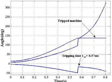
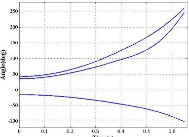
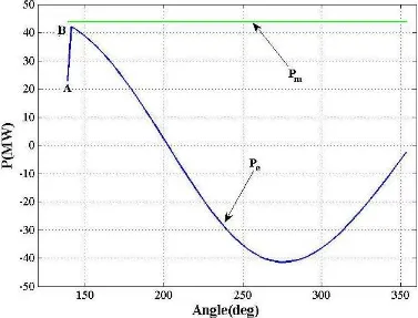
FIGURE 3.5SWING CURVES OF THE INDIVIDUAL MACHINES OF THE EXAMPLE CASE SHOWING THE ACTION OF E-SIME TO STABILIZE THE SYSTEM.AFTER TRIPPING MACHINE 2 ITS ANGLE VALUE

REMAINS CONSTANT... 59

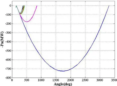
FIGURE 3.6PA-Δ CURVE OF THE OMIB OF THE EXAMPLE CASE SHOWING THE ACTION OF E-SIME TO STABILIZE THE SYSTEM.TIME OF THE DIFFERENT ASSESSMENT AND CONTROL STEPS OF E-SIME ARE INDICATED. ... 59

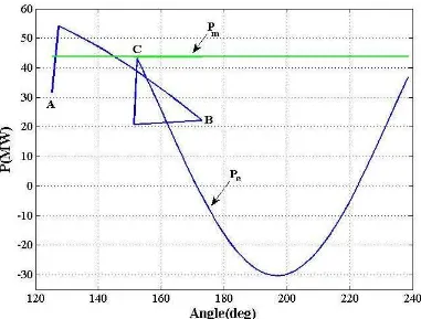
FIGURE 3.7OMIB MECHANICAL AND ELECTRICAL POWERS OF THE EXAMPLE CASE SHOWING THE ACTION OF E-SIME TO STABILIZE THE SYSTEM.POINTS A,B, AND C ARE INCLUDED FOR A STRAIGHTFORWARD COMPARISON WITH FIG.3.5. ... 60

FIGURE 3.8OMIB SWING CURVE OF THE EXAMPLE CASE SHOWING THE ACTION OF E-SIME TO STABILIZE THE SYSTEM.POINTS A,B, AND C ARE INCLUDED FOR A STRAIGHTFORWARD COMPARISON WITH FIG.3.5... 60

FIGURE 3.9OMIB PHASE PLANE OF THE EXAMPLE CASE SHOWING THE ACTION OF E-SIME TO STABILIZE THE SYSTEM.POINTS A,B, AND C ARE INCLUDED FOR A STRAIGHTFORWARD COMPARISON WITH FIG.3.5... 61

FIGURE 3.10GENERIC PMU(ADAPTED FORM [PHADKE,2008]). ... 64

FIGURE 3.11GENERAL FLOW DIAGRAM OF THE E-SIME METHOD COMPUTATIONAL PROGRAM. ... 65

FIGURE 3.12FLOW DIAGRAM OF THE PREDICTION STEP OF INDIVIDUAL MACHINES’ ANGLES. ... 66

FIGURE 3.13FLOW DIAGRAM OF THE COMPUTATION OF THE OMIB PARAMETERS. ... 66

FIGURE 3.14FLOW DIAGRAM OF THE PREDICTION OF THE PA-Δ CURVE. ... 67

FIGURE 3.15FLOW DIAGRAM OF THE EMERGENCY CONTROL ACTION DESIGN STEP. ... 68

FIGURE 3.16FLOW DIAGRAM OF THE COUPLING OF TRANSTAB AND E-SIME PROGRAMS. ... 69

FIGURE 4.1E-SIME STABILITY PREDICTION FOR CASE 1A. ... 74

FIGURE 4.2OMIB EQUIVALENT ANGLE TRAJECTORY BEFORE THE CONTROL ACTION IS APPLIED FOR CASE 1A. ... 74

FIGURE 4.3INDIVIDUAL MACHINES SWING CURVES FOR CASE 1A. ... 75

FIGURE 4.4OMIB EQUIVALENT P-Δ CURVE FOR CASE 1A. ... 75

FIGURE 4.5OMIB EQUIVALENT MECHANICAL AND ELECTRICAL POWERS FOR CASE 1A... 76

FIGURE 4.6OMIB EQUIVALENT SWING CURVE FOR THE CASE 1A:STABILIZED SYSTEM. ... 76

Page

FIGURE 4.8E-SIME STABILITY PREDICTION FOR CASE 2A... 78

FIGURE 4.9INDIVIDUAL MACHINES SWING CURVES FOR CASE 2A... 79

FIGURE 4.10OMIB EQUIVALENT P-Δ CURVE FOR CASE 2A. ... 79

FIGURE 4.11OMIB EQUIVALENT MECHANICAL AND ELECTRICAL POWERS FOR CASE 2A. ... 80

FIGURE 4.11STABILITY PREDICTION FOR CASE 3A. ... 81

FIGURE 4.12Δ–T CURVE OF THE INDIVIDUAL MACHINES AFTER THE CORRECTIVE ACTION FOR CASE 3A. ... 82

FIGURE 4.13P-Δ CURVE OF THE OMIB FOR THE CASE 3A... 82

FIGURE 4.14MECHANICAL AND ELECTRICAL POWERS OF THE OMIB FOR THE CASE 3A. ... 83

FIGURE 4.14E-SIME STABILITY PREDICTION FOR CASE 1NE. ... 85

FIGURE 4.15OMIB EQUIVALENT ANGLE TRAJECTORY BEFORE THE CONTROL ACTION IS APPLIED FOR CASE 1NE. ... 86

FIGURE 4.16INDIVIDUAL MACHINES SWING CURVES FOR CASE 1NE. ... 86

FIGURE 4.17OMIB EQUIVALENT P-Δ CURVE FOR CASE 1NE. ... 87

FIGURE 4.18OMIB EQUIVALENT MECHANICAL AND ELECTRICAL POWERS FOR CASE 1NE. ... 87

FIGURE 4.19OMIB EQUIVALENT SWING CURVE FOR THE CASE 1NE:STABILIZED SYSTEM. ... 88

FIGURE 4.20OMIB EQUIVALENT PHASE PLANE FOR CASE 1NE:STABILIZED SYSTEM. ... 88

FIGURE 4.21E-SIME STABILITY PREDICTION FOR CASE SIEQ... 92

FIGURE 4.22INDIVIDUAL MACHINES SWING CURVES FOR CASE SIEQ... 92

FIGURE 4.23OMIB EQUIVALENT P-Δ CURVE FOR CASE SIEQ. ... 93

FIGURE 4.24OMIB EQUIVALENT MECHANICAL AND ELECTRICAL POWERSFOR CASE SIEQ... 93

FIGURE 4.25OMIB EQUIVALENT SWING CURVE FOR CASE SIEQ:STABILIZED SYSTEM... 94

FIGURE 4.26OMIB EQUIVALENT PHASE PLANE FOR CASE SIEQ:STABILIZED SYSTEM... 94

FIGURE 4.27APPLICATION OF THE E-SIME METHOD TO THE SIEQ TEST SYSTEM. ... 95

Page

FIGURE A.1ONE-LINE DIAGRAM OF EQUIVALENT MMT TEST SYSTEM... 109

FIGURE A.2ONE-LINE DIAGRAM OF THE THREE-MACHINE TEST SYSTEM (ADAPTED FROM [ANDERSON AND FOUAD,1993]). ... 110

FIGURE A.3AUTOMATIC VOLTAGE REGULATOR TYPE 1 MODEL (ADAPTED FROM [PAVELLA ET AL., 2000]). ... 111

FIGURE A.4ONE-LINE DIAGRAM OF THE NEW ENGLAND TEST SYSTEM (ADAPTED FROM [PAI, 1981]). ... 112

FIGURE A.5GEOGRAPHIC DIAGRAM OF THE SIEQ TEST SYSTEM. ... 116

FIGURE A.6SVC BASIC 1 MODEL (ADAPTED FROM [CASTRO,2007])... 116

FIGURE A.7ONE-LINE DIAGRAM OF THE SIEQ TEST SYSTEM. ... 120

FIGURE B.1INDIVIDUAL MACHINES SWING CURVES FOR THE EXAMPLE CASE USING DSATOOLS... 121

L

IST OF

T

ABLES

Page

TABLE 2.1TRANSITIONS BETWEEN OPERATING STATES. ... 26

TABLE 2.2CONTROL MEASURES... 26

TABLE 3.1CLOSED-LOOP EMERGENCY CONTROL OF THE EXAMPLE CASE. ... 56

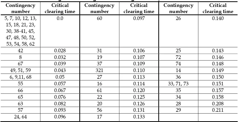
TABLE 4.1CONTINGENCY RANKING OF THE IEEE THREE-MACHINE TEST SYSTEM WITH CLASSICAL MODEL. ... 71

TABLE 4.2CLOSED-LOOP EMERGENCY CONTROL FOR CASE 1A. ... 72

TABLE 4.3CLOSED-LOOP EMERGENCY CONTROL FOR CASE 2A. ... 78

TABLE 4.4CONTINGENCIES RANKING OF THE THREE-MACHINE TEST SYSTEM WITH DETAILED MODEL. ... 80

TABLE 4.5CONTINGENCIES RANKING OF THE NEW ENGLAND TEST SYSTEM WITH DETAILED MODEL... 84

TABLE 4.6CLOSED-LOOP EMERGENCY CONTROL FOR CASE 1NE... 84

TABLE 4.7CLOSED-LOOP EMERGENCY CONTROL FOR CASES 2NE,3NE AND 4NE. ... 89

TABLE 4.8CONTINGENCIES RANKING OF THE NEW ENGLAND TEST SYSTEM WITH DETAILED MODEL... 90

TABLE 4.9CLOSED-LOOP EMERGENCY CONTROL FOR BASE CASE SIEQ. ... 91

TABLE A.1TRANSMISSION NETWORK DATA OF THE MMT EQUIVALENT TEST SYSTEM... 109

TABLE A.2DYNAMIC PARAMETERS OF THE SYNCHRONOUS MACHINES OF THE MMT EQUIVALENT. ... 110

TABLE A.3TRANSMISSION NETWORK DATA OF THE THREE-MACHINE TEST SYSTEM... 111

TABLE A.4DYNAMIC PARAMETERS OF THE SYNCHRONOUS MACHINES AND EXCITERS DATAOF THE THREE-MACHINE TEST SYSTEM. ... 111

TABLE A.5SIMULATIONS USING THE THREE-MACHINE TEST SYSTEM. ... 111

TABLE A.6CONTINGENCIES OF THE THREE-MACHINE TEST SYSTEM. ... 112

TABLE A.7TRANSMISSION NETWORK DATA OF THE NEW ENGLAND TEST SYSTEM... 113

TABLE A.8CONTINGENCIES OF THE NEW-ENGLAND TEST SYSTEM. ... 114

TABLE A.9DYNAMIC PARAMETERS OF THE SYNCHRONOUS MACHINES OF THE NEW ENGLAND TEST SYSTEM... 115

TABLE A.10DYNAMIC PARAMETERS EXCITERS OF THE NEW ENGLAND TEST SYSTEM. ... 115

Page

TABLE A.12TRANSMISSION NETWORK DATA OF THE SIEQ TEST SYSTEM. ... 117

TABLE A.12(CONTINUATION)TRANSMISSION NETWORK DATA OF THE SIEQ TEST SYSTEM... 118

TABLE A.13DYNAMIC PARAMETERS OF THE SYNCHRONOUS MACHINES OF THE SIEQ TEST SYSTEM... 118

TABLE A.14SIMULATIONS USING THE SIEQ TEST SYSTEM... 118

G

LOSSARY

CCT: Critical clearing time.

CIGRE: Conseil International des Grands Réseaux Électriques. CM’s: Critical Machines.

COA: Center Of Angle.

DSA: Dynamic Security Assessment. EAC: Equal Area Criterion.

EEAC: Extended Equal Area Criterion.

DEEAC: Dynamic Extended Equal Area Criterion.

E-SIME: Emergency SIngle Machine Equivalent Method. GPS: Global Position System.

HEEAC: Hybrid Extended Equal Area Criterion.

IEEE: Institute of Electrical and Electronics Engineers. MIPS: Mexican Interconnected Power System.

NM’s: Non-Critical Machines. OLEC: Open Loop Emergency Control. OMIB: One-Machine Infinite Bus. PMU: Phasor Measurement Unit SIME: SIngle Machine Equivalent Method. SPS: System Protection Scheme.

T-D method: Time Domain methods.

TRANSTAB: TRANsient STABility time domain program. WAMS: Wide Area Measurements System.

N

OMENCLATURE

Aacc: Accelerating area.

Adec: Decelerating area. : Rotor angle position.

ct: OMIB angle at control time.

i = (ti): OMIB angle at the current processing time. m: Maximum angular value.

OMIB: OIMIB angle. u: Unstable angle. r: Return angle.

Δt: Sample time. M: Inertia coefficient.

η: Transient stability margin. Pm: Mechanical power.

Pe: Electrical power.

Pa: Accelerating power.

Pep: Post-fault electrical power.

t0: Is the beginning of the during-fault period of the time.

te: Is the beginning of the post-fault period of the time.

tf: Time at what the predictive TSA starts.

ti: Current processing time.

tct: Is the passed by time between the occurrence of the contingency and

the control action; it is also called “the control time”.

td: Is the total time of the program to acquire the data, transmit the

control order to the power plant and to apply the control action. tu: Time to instability of the system.

ω: Rotor speed.

C

HAPTER

1:

I

NTRODUCTION

1.1 INTRODUCTION

The electricity supply is one of the basic and most important resources that countries have, it has a very important role in modern economies since they have a strongly dependence on reliable and secure services [Knight, 2001, CIGRE, 2001].

Electric power systems must be designed to supply an electric energy service at minimum cost with the least impact to the environment. They must maintain the level of reliability, quality and security of the system, and simultaneously find a new balance of energy flows while optimizing the generation and coordinate control actions of the control areas involved in the system [Fink and Carlsen, 1978, Kundur, 1994]. To achieve this, systems must operate in an efficient way at normal operating conditions, and after the occurrence of any disturbance, they must be capable of absorbing these stresses without further damage. When disturbances take place, the operating conditions change, and it is necessary to carry out control measures in order to successfully bring the system back to its normal operation state, depending on the security level.

Historically, power systems have been widely interconnected in order to supply electricity to the customers in a reliable and secure way, or to interchange power in emergencies [Fortesque, 1925, Elgerd, 1982, Kundur, 1994]. Over the years, operation of power systems has changed according to the necessities of the electric industry, from the isolated operation to supply individual loads, till the interconnection of wide areas forming pools in one system or between systems. This latter was achieved with the development of the alternating current transmission of power and the parallel operation of generators started approximately in 1890 [AIEE, 1937] and has been largely developed until these days.

Apart from the inherent problems of the system operation, in some systems in which electric utilities have been restructured, creating electric markets [Hunt y Shuttleworth, 1996], [Pérez-Arrillaga, 1982], new problems related to the specific characteristics of these markets have been emerged such as the problem of transmission system expansion, which in turn additionally decreases the power transmission capacity. In these very limited conditions, it is necessary to implement discrete stability controls; without which power systems could not operate at the current transmission levels required nowadays.

The most common transient stability protection schemes used in these days are based on the occurrence of a specific event and are designed and adjusted by means of off-line studies. However, in the real operation of the system, operators may find unpredicted operating conditions that were not taking into account in the design studies; in consequence it is possible that in some occasions protection devices would fail.

Due to this fact, it has been proposed to use more intensely system protection schemes employing real time measurements. This trend has been reinforced by the growing development of systems that provide fast synchronized measurements in real time. This is the reason this work studies the Emergency SIngle Machine Equivalent (E-SIME) Method, an approach which allows implementing system protection schemes to solve transient stability problems using real time measurements.

1.2 OBJECTIVE OF THE THESIS

1.3 HISTORICAL BACKGROUND AND MOTIVATION

This section presents a literature review related to the main subject of this work, the Single-Machine Equivalent method (SIME) and its two variants: the “preventive SIME” and the “emergency SIME”. This method, and in particular E-SIME are described in chapter 3.

1.3.1 The SIME method

SIME is a hybrid direct-temporal transient stability method. It is based in the combination of time domain simulations with the Equal Area Criterion (EAC), which has been widely studied and strengthened over the time.

In [Skilling and Yamakawa, 1940] the EAC was used to determine the transient stability limits and to reduce the complete system to a One Machine Infinite Bus (OMIB) equivalent system. In this paper, a graphic method is proposed as an extension of the EAC developed before in [Dahl, 1938] and permits it to be applied to analyze power system stability under disturbances in which time is an important factor. Its main advantage is that it allows determining the angular position of the synchronous machine as a function of time; i. e., that the swing curve can be plotted from these results. From that time on, EAC was considered as a method that could only be applied in small systems that could be simplified to a two-machine system represented with the classical model.

In [Xue, 1988, Xue et al., 1988] authors proposed an uncomplicated direct method for power system on-line transient stability assessment based on the combination of the OMIB equivalent with the EAC and combining it with Taylor series expansions and corrective factors in order to amplify the advantages of Liapunov’s direct approaches. The proposed method was called the Extended Equal Area Criterion (EEAC) and consisted of decomposing of the multimachine system into two groups: the “candidate critical machines” and the remaining machines, and to aggregate them into an equivalent OMIB system; then the “pre-filter” candidate critical machines are tested in a sequence to identify the critical ones. With this method, the analysis of transient stability was performed free from step-by-step calculations or trial and error procedures, and stability margins are calculated in an analytical fashion.

Latter, in a subsequent work [Xue et al., 1993] the EEAC is presented as a new direct method to adapt the EAC to multimachine fast transient stability assessment by decomposing the system machines into two re-named groups: the critical cluster (CC1_{) and the one that comprises the rest of the machines, then aggregate each group}

into an equivalent machine and replace the resulting two equivalents by an OMIB system in order to apply the EAC to this OMIB.

At the beginning of the EEAC development, the CC’s selection was based on the “initial accelerations criterion”, in other words: machines likely to be critical are considered those with the largest initial accelerations, but these variables do not reflect the actual degree of machines’ criticalness. This first version of the EEAC proposed in [Xue et al., 1993] gave very good results with a large variety of power systems (for instance, the Chinese EMS and the French EHV systems). However, some difficulties were revealed and they introduced two changes: the individual angles were refreshed during and after the fault (Dynamic OMIB) and the critical machines are classified in the proper order they should be combined. Then the EEAC evolved into the Dynamic EEAC (DEEAC) [Xue et al., 1993] which gradually gave rise to the Hybrid EEAC (HEEAC) [Zhang, 1995], which was subsequently renamed as the SIME method [Zhang et al., 1997, Pavella et al., 2000].

The main assets that SIME provides are: an early termination stopping criterion (which consequently reduces of the length of the required time domain simulations), the assessment of stability margins and the possibility of identifying the group of critical system machines. In [Zhang et al., 1996] the most important rules and steps to implement SIME method were presented. These five rules are the fundamentals of SIME and state the general approach to formulate the OMIB system in an appropriate fashion and to calculate the stability margins (positive for stable scenario, zero for the borderline stability case and negative for unstable scenario) then the aggregation of the relevant machines (CC) and the remaining ones into the relevant OMIB system.

In [Zhang et al., 1996] it was also presented the application of the SIME method to the Hydro-Québec System for first swing and multi-swing stability assessment. The SIME method has been also tested on the Brazilian network that is a system that required an accurate method to screen contingencies in order to identify only the relevant ones and, at the same time, provide accurate results for the secure operation of the system [Bettiol et al., 1997] and proved to be a successful method that is computationally efficient and has the ability to handle any power system with all kinds of modeling. In [Bettiol et al., 1997] it was also proposed a variant of SIME method: “filtering SIME” that deals with the selection of contingencies that would provoke instability.

1 _{The CC contains the critical machines that are responsible for the separation of the system whenever}

Filtering SIME consists basically in the selection of the “potentially harmful” contingencies and the rejection of the “harmless” ones; the purpose of this latter is to become faster but preserve the reliability of the method and these conditions can only be reached by relaxing the strict accuracy requirements of SIME while selecting the contingencies. The final procedure is integrated by a sequence of the filtering phase (consisting in two filtering steps) and the contingency assessment phase. In the Brazilian South-Southeast power system of 56 generators, the filtering SIME was carried out using simple and detailed modeling and a list of 192 contingencies. In the filtering phase, the first step rejected 127 contingencies and “sent” 65 to the second filtering step where filtering SIME discarded other 55 contingencies and selected only 10 feasible contingencies to be assessed by regular SIME.

Gradually, SIME has been divided into two types of transient stability assessment: preventive and predictive transient stability assessment. In general, preventive control aims at assessing “what to do” in order to avoid loss of synchronism if an a priori harmful contingency would occur while the emergency control aims at triggering a countermeasure in real time after a contingency has actually occurred [Ernst et al., 2000, Ernst and Pavella, 2000]. This latter type of control has been implemented in two fashions: “open-loop emergency control” and “closed-loop emergency control”.

SIME was initially developed to improve the performance of the conventional time-domain (T-D) techniques for transient stability assessment and was extended to embrace preventive and emergency control and originated two types of SIME method: “Preventive SIME” that goes on the traditional way of assessing transient stability and “Emergency SIME (E-SIME)” that uses real time measurements to assess transient stability [Ernst et al., 2000].

1.3.2 The E-SIME method

In [Ernst et al., 2000] an approach to the preventive and emergency transient stability control schemes using SIME was presented.

Latter on, the emergency SIME method has been studied in different fashions and has been modified and strengthened. In [Ruiz-Vega et al., 2003] it was proposed a combination of two powerful techniques for emergency control: the closed-loop emergency control (E-SIME) and the open-loop emergency control (OLEC) in different horizons of time to combine preventive with emergency actions. In a more recent work the main purpose is to use the same general SIME-based method and combine their desirable features: the quickness of the OLEC action and the closed-loop capability of E-SIME [Ruiz-Vega et al., 2003].

method. They use a generation shedding scheme as a control action to avoid instability that has been tested in various real-life power systems like the South-Southeast Brazilian system, the EPRI test system, the WECC system and Hydro-Québec system using the ST-600 and ETMSP programs as TD simulations as a base for E-SIME just for want of real-life measurements. Providing the emergency scheme would become strongly system dependent, they also recommend the evaluation of various different types of control actions instead of using the generation tripping only. Some conclusions and observations are presented in order to enable the reader to take into consideration the system conditions like the angle reference and external conditions like noise and the number of measurements.

The Single Machine Equivalent method has been the subject of large research and some books are concentrated on the power systems security assessment and deals with the crux of SIME: The Book [Pavella et al., 2000] presents a comprehensive approach to transient stability assessment and control. Here is presented the development of SIME method and its variants over the time and the techniques to implement the procedure. The two different methods are the “Preventive SIME” and the “Emergency SIME” so this book is mainly divided into these two approaches. Some other books or chapters of books devoted to this topic are: [Wehenkel et al., 2006] [Ruiz-Vega and Pavella, 2008] and [Pavella et al., 2009].

1.4 JUSTIFICATION

The growing competition in the electric power utility environment has resulted in an augment of stress in transmission systems [Karady and Gu, 2002]. In the current power systems, especially those in which an electric market has been established and where the active power is viewed as a product to commercialize, the preventive control schemes for the security of power systems, mainly consisted in the security constrained re-dispatch, are every time less accepted and as a consequence there have been proposed system protection schemes consisted in executing emergency controls when a large disturbance affects the system [CIGRE, 2001].

in this work, the emergency- single machine equivalent method (E-SIME), provides the basis for developing a measurement-based system protection scheme, which is able to stabilize the system using a generation tripping control action.

1.5 SCOPE

At this stage of the research, this thesis work deals exclusively with the description and performance evaluation of the emergency SIME method in predicting transient stability and designing control actions early enough to be able to stabilize the system using generation tripping schemes.

The practical application of the method is limited by the current development of the communication systems and the PMU’s installed in the network, because these units can not provide the measurements at the required sampling and speed. Moreover, PMU’s only measure voltage and current phasors at the transmission system level, while the necessary variables to develop the method (load angles, machine speeds, mechanical powers and electrical powers) can not be provided yet.

As a consequence, in this work the results of a computational program are used to simulate the real time measurements. However, as described in the following section, important contributions have been made in this work in order to arrive towards the method practical implementation.

1.6 CONTRIBUTIONS

The main contributions of this work can be briefly described as follows:

• A detailed description of the emergency SIME method and of its two main steps: the predictive transient stability assessment and the design of control actions using generation tripping schemes, is presented.

• The development of a new computer program to automatically apply the E-SIME method. The program was coupled with the TRANSTAB time-domain simulator, but it was developed as an independent module that in a near future can be used with more powerful time-domain simulators in the testing phase of the method, and as the basis for a future program using real-time measurements.

the method is able to work in cases where the contingencies affect meshed power systems where the critical machines cannot be easily known in advance.

• A new equivalent test power system was developed in order to use a more realistic system to test the E-SIME method. This power system was derived from the Oriental Control Area of the Mexican Interconnected Power System of 2001, and was selected because various power plants in this system are equipped with event-based automatic tripping schemes.

1.7 PUBLICATIONS DERIVED FROM THE THESIS

• Laura. L. Juárez Caltzontzin, Daniel Ruiz Vega (2010). “Predictive Evaluation of Transient Stability Using the Emergency SIngle-Machine Equivalent Method” (in Spanish). Memorias de la Reunión de Verano de Potencia del IEEE, July 11 to 17, 2010. Acapulco, Gro., MEXICO.

1.8 THESIS ORGANIZATION

This section outlines the main structure of the thesis, as follows:

• Chapter 1 presents an introduction to the topic of research, the objective and scope of this thesis, and the reasons for the developing of this work and its contributions.

• Chapter 2 outlines and discusses the main methods for controlling transient stability problems, including generation tripping schemes.

• Chapter 3 describes in detail the Emergency SIngle-Machine Equivalent E-SIME method and its two main steps: predictive transient stability assessment and control design. The structure of the developed program and its coupling with the time-domain simulator are outlined. Some requirements for its future practical application are also mentioned.

• Chapter 4 shows the application of the methodology to different power systems, showing cases in which the method is able to control transient stability by itself and where it needs to be combined with an automatic system protection scheme.

C

HAPTER

2:

T

RANSIENT

S

TABILITY

C

ONTROL

2.1 INTRODUCTION

Security is the robustness of the power system in terms of its ability to withstand a wide variety of disturbances (programmed or not) and to operate in equilibrium under normal and distressed conditions, while reducing the risk of outages [Dy Liacco, 1978, Knight, 2001, Kundur, 1994, Pavella et al., 2000, IEA,2005].

For the purpose of security, the power system is planned and operated to maintain the following conditions [Ruiz-Vega, 2002b, Kundur, 2000]:

• After any disturbance, any element of the system is overloaded (static condition).

• After any disturbance, all bus voltages are within their permissible limits.

• After any disturbance, the system must be stable and during the transient period it must have an acceptable voltage drop and damping.

The first two conditions are studied in static security; the third condition is the main concern in this work and belongs to the field of dynamic security assessment and control.

In addition to the conditions described above, the power system planner and operator must take into consideration some other aspects for instance: the constant change of the global economy, the growing awareness of natural environment and the restructuring of electric utilities where economic aspects must be taken into account to minimize looses and augment the earnings. The horizon is not flexible at all: the majority of the decisions are made in a context of uncertainty (the demand, the availability of the resources to produce energy, the prices, the fuel, the regulatory legislation, etc.) [Expósito, 2009]. Thus, in the widest framework, the power system must be able to maintain the load demand of power and should supply quality environmentally friendly energy at the lowest prize within its permissible limits.

To achieve all those functions, the power system requires the employment of a coordinated hierarchical control system [Dy Liacco, 1978] flexible enough to avoid wrong interactions that could cause adverse situations such as power system oscillations or instabilities. However, these control systems are very complicated because they are based on a great quantity of measurements that are continually monitored and actualized. As a consequence, the majority of these control schemes are performed by powerful computers in energy management centers [Expósito, 2009].

Power system operation and control has been unfolded over the years, its development is predominantly the result of the study of the blackouts occurred worldwide. In Fig. 2.1 it is shown the evolution of power system control technology over the years.

1950 1960 1970 1980 1990 2000 2003

Automatic Generation Control; Analog Computer Utilization

for Economic Dispatch

Local Monitoring and Control Static Mimic Board; Telephone Commands

Analog Data Acquisition System

Digital Transmission Supervisory Control and Data

Acquisition (SCADA)

Digital Computer Utilization for Off-line Studies

Development of Optimal Power Flow

Load Management (Ripple Control) Development of State Estimation Integrated SCADA/EMS Process Computers

for SCADA Functions; Video Display Units

1965 1977 1983 1996

Emergency State Control; Emergency and Restorative

Actions 1982 Chilean Electric Industry Liberalization Dispatch Trainning Simulators Distribution Automation; Demand and Supply Side

Load Management GUI Using Full Graphics Optimal Security Constrained Power Flow Development of On-line Dynamic Security Assessment and Control New Market-Oriented EMS Applications Development of System Monitoring Using Phasor Measurements US Northeast System blackout New York blackout Sweden voltage instability US WSCC blackout American and European blackouts 1940

Figure 2.1 Significant events in the evolution of power system control technology [Ruiz-Vega, 2009]. Adapted from [Handschin and Petroianu, 1991] and Updated from [Ruiz-Vega, 2002a].

using the telephone to send commands to the field system operators. The automatic generation control was made in an analogue fashion. In general, the progress in power system monitoring and control is the result of the improvement in other fields like: computation, electronics, signals processing, measurement devices, etc. With the development of the acquisition data systems, the monitoring and control of the power system evolved and computers were used for off-line power system planning studies [Handschin and Petroianu, 1991].

With the occurrence of the New York blackout in 1965, the concern about the importance of the security assessment started to grow, and during the seventies, the State Estimator and optimal power flow theory had their main improvement. Later, in the eighties, after a new series of blackouts and with the advent of computer hardware able to manage with the system, the necessity of trained operators was evident and training simulators were carried out [Handschin and Petroianu, 1991].

In this context, the security assessment of power systems becomes an important challenge for power system’s planners and operators since any power system (even if it is designed to withstand any “plausible” contingency) is a potential candidate to be threatened by a disturbance (whatever its nature) that may led to a partial or total collapse of the interconnected system.

This problem has not been caused by isolated conditions, it may be seen as the consequence of several factors: as power systems have growth in interconnections, new technologies and controls have emerged, in addition, power systems operate every time more stressed and nearest their stability limits. In some industries, were the electric utilities have been reformed, it has been demonstrated that the security of the transmission network is vital in the operation of electricity markets and recent 2003 disruptions in America and Europe (see [IEA, 2005]) have created concern that electricity reform had reduced electricity system reliability [IEA, 2005], all these conditions have also provoked the emerging of different forms of system instabilities [CIGRE, 2000] that will be introduced in § 2.2.

2.2 POWER SYSTEM STABILITY

Figure 2.2 Measured values of the Mexican National interconnected power system during two different days in two different seasons in 1995 (Adapted from [Ruiz-Vega, 2002a]).

Power system stability has been widely studied over the years and has been recognized as an important problem for secure system operation since the 1920s [IEEE, 2004]. Historically, it started giving cause for concern with the parallel operation of synchronous machines around 1890 [AIEE, 1937] where first stability problems were spontaneous oscillations or “hunting” due to inefficient damping that were solved by introducing damping windings and turbine-type prime movers [Concordia, 1985]. However, it was up to the latest fifties when the majority of the problems were encountered to be transient instabilities [Ruiz-Vega, 2002b].

With the interconnection of power systems, new types of instability such as voltage instabilities, frequency instabilities, etc., started being studied what made necessary the punctual definition and classification of power system stability. In [IEEE, 2004] power system stability is defined as the ability of an electric power system, for a given initial operating condition, to regain a state of operating equilibrium after being subjected to a physical disturbance, with most system variables bounded so that practically the entire system remains intact. This definition is valid for the entire system, which means that if a single generator or group of generators losses synchronism2 _{the system as a hole}

would remain stable.

This definition assumes that during the transient period, between the initial stationary state (pre-disturbance) and the final stationary state, the damping and the main variables of the power system are within their admissible limits and have little impact on the quality of the electric service. The final operation state of the system must be acceptable so that their frequency and voltage values remain within their normal limits and all the generators operate in synchronism [Ruiz-Vega, 2002b].

2.2.1 Power system stability classification

The classification of power system stability is shown in figure 2.3 and is based on different aspects of the power system [IEEE/CIGRE, 2002]:

• The physical nature of the instability that is indicated by the main variable affected by instability (rotor angle, frequency or voltage).

• The size of the disturbance (large or small).

• The devices, processes and times that must be taken into account to assess stability

Power System Stability

- Ability to remain in equilibrium - Equilibrium between opposite forces

Frequency Stability Small Signal Stability (Small disturbances ) Rotor Angle Stability Voltage Stability Transient Stability (Large disturbances ) - Ability to maintain synchronous operation - Balance between electric and

mechanic torques in synchronous machines

- Ability to maintain frequency within its nominal range - System generation /load balance

Short term Long term

- Ability to maintain voltage within acceptable values - Dynamic load restoration

Small Disturbance Voltage Stabiltity Large Disturbance Voltage Stability

Short term Long term Short term

CONSIDERATION FOR THE CLASSIFICATION

Physical Nature / main parameter

Size of the Disturbance

Time Span

Figure 2.3 Power Systems Transient Stability Classification (Adapted from [IEEE, 2004]).

Here there are presented the definitions of the different types of stability based on the physical nature of the instability:

Rotor angle stability: is the ability of the synchronous machines of an interconnected

Frequency stability: is the ability of the power system to maintain the frequency within a normal range after being subjected to any disturbance resulting in a significant imbalance between generation and load that could (or not) lead to the separation of the interconnected power system in isolated subsystems.

Frequency stability depends on the ability of the power system to restore the total of the generating power and the load power balance in the different subsystems with minimum loss of load [Kundur and Morrison, 1997].

Voltage Stability: is the ability of the power system to maintain steady voltages at all

buses in the system after being subjected to a disturbance [IEEE, 2004]. This stability type depends on the ability of the generation and transmission power subsystems to restore the load power and reach acceptable voltage values in all the nodes of the system after a disturbance. The voltage instability is the result of the load effort to restore the energy consumption to a greatest value that is the combined capacity of the generation and transmission subsystems [Van Cutsem and Vournas, 1998].

Based on the size of the disturbance, stability is classified as follows:

Small disturbance or small signal stability: is the ability of the power system to

remain in synchronism after being subjected to a small disturbance.

A disturbance is considered small if its consequences could be examined by a linear model of the system, otherwise the disturbance can be classified as a large disturbance [IEEE, 2004]. What defines the size of a disturbance are the techniques employed to solve the mathematical problem, the results of an analysis using the linear model of the system must be valid for the real system (non-linear system). Analysis techniques using linear and non-linear models are supplementary and the identification of the causes and their possible solutions require a coordinated usage of both. Despite the fact that linear techniques are highly attractive because of their advantages (like the availability of sensitivity techniques able to identify the elements that provoke the instability and those which have an important influence in the phenomena) their results are not always valid for the real system [Ruiz-Vega, 2005].

Large disturbance or transient stability: is the ability of the power system to

maintain synchronism when it is subjected to a large disturbance (for instance a short circuit), the response of the system has to do with large excursions of generator angles. This thesis is devoted to transient stability and a deep analysis on it is made in § 2.2.2 and chapter 3.

Based on the time span the classification of stability is:

Long term stability: the phenomena of interest are in the period of time from

Short term stability: the phenomena of interest are in a period of time from tens of seconds to tens of minutes (slower phenomena).

In figure 2.4 it is shown the time span of the different types of instabilities that occur in the power system. It can be noticed that the different kinds of instabilities defined above have different and specific periods of time. Thus, transient instabilities are developed in periods of time up to 20 seconds (short term stability) while frequency and voltage instabilities can be classified in both short and long term stability for any size of the disturbance.

2.2.2 Power system instability classification

Depending on the network topology, system operating conditions and the form of disturbance, different sets of opposing forces may experience sustained imbalance leading to different forms of instability [CIGRE, 2007]. In this context, transient instability can be also classified as follows [Ruiz-Vega, 2002b]:

First swing stability: is the result of the lack of synchronizing torque and results in an aperiodic change of direction in the rotor angle of the group of machines that loses synchronism.

10−7

10−4 10−5

10−6 10

3

−

10−2 10−1

1 10 10210

3

106 104

105 ₁₀7

Time scale (s)

Lighting overvoltages

Line swithching overvoltages

Subsynchronous resonance

Transient and small signal stability

Long term stability

Frequency regulation

Daily load following

1 µs

1 degree at 60Hz 1 cycle 1 minute 1 hour 1 day

Multi-swing stability: is the result of the lack of damping in the system and results in an oscillatory instability.

The second classification of transient instability is made in terms of the group of machines that loses synchronism [Ruiz-Vega, 2002b].

Up-swing stability: this kind of instability occurs when the accelerating machines’

group loses synchronism.

Back-swing stability: this kind of instability occurs when the decelerating machines’

group loses synchronism with respect to the others.

The third classification of transient instability is made as a function of the number of machines that lose synchronism [Ruiz-Vega, 2002b].

Plant mode instability: this phenomenon is presented when one or more machines of

the same power plant lose synchronism.

Inter-area mode instability: Is presented when an important group of machines loses

synchronism with respect to the rest of the system.

2.3 TRANSIENT STABILITY

Transient stability may be defined as the ability of a power system to maintain the synchronous operation of synchronous machines when it is subjected to a large disturbance (physical approach). However, power system transient stability is similar to the stability of any dynamic system which has a mathematical description so that power system transient stability is a strongly nonlinear high dimensional problem (system theory approach) [Pavella et al., 2000].

If one generator of the power system goes faster than another, the angular position of its rotor relative to that of the slower machine will advance. These angular difference shifts part of the load from the slower machine to the faster machine to reduce the speed deviation and the angular separation. In spite of the fact that the power-angle relationship is strongly nonlinear, after a certain limit, this angular difference causes the power transfer to decrease and the angular separation to increase. If the system restoring forces are capable of maintaining the machines in synchronism absorbing the kinetic energy corresponding to these rotor speed differences after the fault time clearance then the system will be stable, otherwise the system will lose synchronism. [Kundur, 1994, Kimbark, 1948].

Loss of synchronism would occur between one machine and the rest of the system, or between groups of machines, with synchronism maintained within each group after separating from each other [IEEE, 2004].

The torque deviation of a synchronous machine after being subjected to a disturbance can be separated in two components (equation 2.1) [Kundur, 1994] and system stability depends on the existence of both of them [IEEE, 2004].

ω

δ + Δ

Δ =

ΔT_e T_S T_D (2.1)

Where:

Δ is the synchronizing torque component and TS is the synchronizing torque

coefficient, thenTSΔ is the component torque in phase with the rotor angle deviation.

And Δω is the damping torque component and TDis the damping torquecoefficient,

then TDΔω is the component torque in phase with the speed deviation.

In the absence of sufficient synchronizing torque aperiodic or nonoscillatory instabilities would occur and lack of damping torque leads to oscillatory instabilities [IEEE, 2004].

t

V

V

Infinite Bus

TR

X

1

TL

X

2

TL

X

Figure 2.5 One-machine infinite bus system (Adapted from [Kundur, 1994]).

The dynamic model of this OMIB system consists in a single equation (2.2): the swing equation.

2

m e a d

M P P P

dt δ

= − = (2.2)

That is usually divided into two differential equations:

m e a

d

M P P P

dt ω

= − = (2.3)

0 d

dt δ

ω ω

= − (2.4)

Where:

M= the inertia coefficient = the rotor angle position ω =the Rotor speed

Pm= the mechanical power

Pe= the electric power

Pa= the accelerating power

The system can be represented by the “classical model” which is adequate to analyze first swing stability and is the simplest representation of it. Classical model dynamics are described by equation (2.2) and other considerations for modelling are [Kundur, 1994, Kimbark, 1948, Anderson and Fouad, 1977]:

• Machines are represented by an mmf behind the direct axis transient reactance.

• Loads are represented by a constant impedance model.

• The mechanical power is constant and damping is neglected.

t

V

eq

X

V

Infinite Bus

Figure 2.6 Basic one-machine infinite bus system.

The transient stability problem can be solved in different fashions and in the following section there will be presented two approaches to deal with transient stability.

2.3.1 Transient stability approaches.

TD-Approaches

As power system grew in size and interconnections, they could no longer be represented by an OMIB system; with the interconnection of power systems, new stability problems emerged and the modelling requirements to represent the system evolved too, generators and excitation systems’ mathematical representation rose in detail and complexity and new methods to assess stability were employed: the time-domain (TD) methods of integration; TD methods started being popular with the advent of computers because they allow the representation of the dynamic behaviour of the system closer to its real functioning making possible to include detailed models of the elements involved in the system (generators, loads, the transmission network and some other dynamic devices) and to represent the non-linearity of the system. TD methods have two main features [Ruiz-Vega, 2009]:

• The time-domain simulation results are able to accurately predict the dynamic behaviour of the system but it depends on the precision of the parameters employed.

• They are not capable of providing sensitivity techniques to determine the causes of the stability problem and design adequate control measures.

In consequence most of the investigations and researching efforts are devoted to develop some aspects of the TD methods.

In TD methods, the model of a multi-machine system is divided into two sets of equations:

) , (x y f

x⋅ = (2.5)

) , (

0=g x y (2.6)

differential equations that represent other dynamic elements and their controls. The set (2.6) represent the algebraic equations of the machines’ stator, the network, and loads.

The TD approach simulates the system dynamics in the during-fault period and post-fault configurations. The during-post-fault period of simulation is very short while the post-fault period of simulation is longer [Pavella, et al., 2000].

The sets of equations (2.5) and (2.6) must be co-ordinately solved, for that purpose, different schemes of solution have been proposed that depend on the integrating method chosen, the two main methods are:

• Alternate-Explicit method

• Simultaneous-Implicit method

The Alternate-explicit method was the first method proposed for time simulation. The use of an integration method allowed solving equation systems (2.5) and (2.6) in an alternate fashion. The values of the state variables of the system are found by an explicit integration method (for instance: a Runge-Kutta method) in a single step without interacting with the network solution. This latter is due to the fact that in the moment of computing the differential equations, the network variables are considered constant and vice versa: during the network equations solution, the state variables of the system are considered constant.

When a disturbed is applied to a power system, the set of equations (2.6) has to be resolved again to obtain the new values of the algebraic variables. The state variables do not need to be recalculated because the have no discontinuities [Ruiz-Vega, 2009]. In spite of its simplicity, the Alternate-explicit methods were preferred at the beginning of the development of digital computer programs, this was possible because the power system could be represented by a classic model and the first-swing stability studies were the most common.

Nevertheless, approximately in the sixties, the usage of excitation controls of fast responses started to be generalized and the interconnection of power systems caused the appearing of poor damped low frequency oscillations or instable oscillations. In order to avoid this situation the representation of the system had to be improved and the level of modeling augmented to reproduce the system behavior in a wide time horizon (say 20sec.) for the purpose of proving the effectiveness damping of the system oscillations.

instabilities [Arrillaga and Arnold, 1990] and caused the method to become impractical. This lead to the development of new kinds of methods, mainly those that use implicit integration methods (for example: trapecial rule) and in the latest of the sixties and during the seventies the simultaneous-implicit methods emerged. Nowadays, these TD methods continue being the most accepted for TSA.

TD methods have many advantages and disadvantages, some of them are [Pavella et al., 2000]:

Pros of TD methods:

• They give the dynamic description of the system’s behavior in the time domain.

• Any power system with different degree of modeling can be studied.

• Is very accurate when the parameters are precise enough.

Cons of TD methods:

• Do not provide tools to throw away the harmless disturbances for the system under study.

• They can not provide stability and security margins.

• They are helpless in the design of control actions to improve stability.

Direct approaches

Another way to attempt TSA is using direct methods that started being developed in the sixties. Its main features are: the restriction of the TD simulation only for the during-fault period (what avoids the repetition of TD simulations and computer effort) and the possibility of obtaining stability margins [Pavella et al., 2000].

One of the most difficult tasks to apply direct methods is the construction of good Lyapunov functions for multimachine power systems what is only possible if very simplified models of the system are used. Another difficult is the assessment of a practical stability domain. These difficulties were overcome by combining theoretical approaches with practical engineering solutions.

2.3.2 Transient stability assessment using the EAC.

The EAC is a powerful technique to assess power system transient stability. As it was mentioned in chapter 1, their origins are not clear but first proposals were made in [Dahl, 1938, Crary, 1947, Kimbark, 1948]. This method allows the study of the behaviour of a one-machine system connected to an infinite bus without solving differential equations.

Considering the OMIB system in figure 2.5 with the features mentioned before, and which is governed by equation (2.2) we can multiply both sides this equation by d /dt [Pavella et al., 2000]:

2

a

d d d

M P

dt dt dt

δ δ δ

= (2.7)

Therefore.

2

2 a

d d

M dt d

P dt dt δ δ    

  _{= (2.8)}

Multiplying by dt to have differentials:

2

2 a

M d

d P d

dt δ δ   =  

  (2.9)

Integrating (2.9) between 0 (the pre-fault equilibrium angle) to (any post-fault

angle): 0 2 2 a M d P d dt δ δ δ δ   =  

 



Or in terms of equation (2.4):

(

)

ω ω− =



Thus. 0 0 2 a P d M δ δ

ω ω− =



Here ω - ω0 is the relative speed of the machine respect to the infinite bus. Providing

this speed return to zero the system will be first-swing stable then the speed will return to zero if the accelerating power is either zero or opposite sign to the rotor speed. An increasing in rotor angle implies that the difference ω - ω0is greaterthan

zero, when the rotor angle reaches its maximum value ( m) then the difference ω - ω0

equals zero. This happens when a negative accelerating power Pa damps the speed

0

0 P da 0; 0 m

δ

δ

ω ω− =



0

0 0; ( ) 0

m

a a m

P d P

δ

δ

ω ω− =



In order to assess transient stability by means of the EAC to a multimachine power system it is necessary to simplify it to a two-machine equivalent system and then replace it by an equivalent OMIB (see § 3.2.2) that represents the dynamics of the entire system. The application of this criterion to assess transient stability of a power system will be done in chapter 3.

To illustrate the EAC, let us consider that in a system like the one displayed in figure in figure 2.5 has been subjected to a three-phase fault at bus A, the initial operating point of the system is the intersection of mechanical and electric power (point 1 in figure 2.7). Due to the disturbance, the electric power transfer falls to zero (point 2) at this point the electric power is smaller than the mechanical power and the machine gains kinetic energy until the fault is cleared at point 3, the system reaches point 4 the area 1,2,3,4 represents the accelerating area of the system. When the fault is cleared, the system reaches u and the system conditions changes to curve Pep. EAC states that

the system will be stable if the decelerating area is at least equal to accelerating area. In order to achieve this latter there are a wide variety of control actions to stabilize the system and become the decelerating area greater then the accelerating one. These control schemes will be fully described in § 2.4.