Econometría Michael Creel (2014)

(1)

Econometrics

Michael Creel

Department of Economics and Economic History

Universitat Autònoma de Barcelona

(2)

List of Figures

1.1 Octave . . . 19

1.2 _LYX . . . 20

3.1 Typical data, Classical Model . . . 31

3.2 Example OLS Fit . . . 34

3.3 The fit in observation space . . . 35

3.4 Detection of influential observations . . . 40

3.5 Uncentered R2 . . . 43

3.6 Unbiasedness of OLS under classical assumptions . . . 48

3.7 Biasedness of OLS when an assumption fails . . . 49

3.8 Gauss-Markov Result: The OLS estimator . . . 53

3.9 Gauss-Markov Resul: The split sample estimator . . . 54

5.1 Joint and Individual Confidence Regions . . . 91

5.2 RTS as a function of firm size . . . 105

7.1 s(β) when there is no collinearity . . . 125

(12)

7.2 s(β) when there is collinearity . . . 126

7.3 Collinearity: Monte Carlo results . . . 130

7.4 OLS and Ridge regression . . . 136

7.5 ρˆ−ρ with and without measurement error . . . 142

7.6 Sample selection bias . . . 146

9.1 Rejection frequency of 10% t-test, H0 is true. . . 172

9.2 Motivation for GLS correction when there is HET . . . 188

9.3 Residuals, Nerlove model, sorted by firm size . . . 193

9.4 Residuals from time trend for CO2 data . . . 201

9.5 Autocorrelation induced by misspecification . . . 203

9.6 Efficiency of OLS and FGLS, AR1 errors . . . 213

9.7 Durbin-Watson critical values . . . 220

9.8 Dynamic model with MA(1) errors . . . 224

9.9 Residuals of simple Nerlove model . . . 225

9.10 OLS residuals, Klein consumption equation . . . 228

10.1 Exogeneity and Endogeneity (adapted from Cameron and Trivedi) . . . 236

11.1 Search method . . . 286

11.2 Increasing directions of search . . . 289

11.3 Newton iteration . . . 292

11.4 Using Sage to get analytic derivatives . . . 296

11.5 Mountains with low fog . . . 302

(13)

12.1 Effects of I_∞ and J∞ . . . 329

13.1 Dwarf mongooses . . . 368

13.2 Life expectancy of mongooses, Weibull model . . . 369

13.3 Life expectancy of mongooses, mixed Weibull model . . . 371

14.1 Method of Moments . . . 377

14.2 Asymptotic Normality of GMM estimator, χ2 example . . . 388

14.3 Inefficient and Efficient GMM estimators, χ2 data . . . 392

14.4 GIV estimation results for ˆρ−ρ, dynamic model with measurement error . . . 412

14.5 OLS . . . 423

14.6 IV . . . 424

14.7 Incorrect rank and the Hausman test . . . 429

15.1 NYSE weekly close price, 100 ×log differences . . . 461

15.2 Returns from jump-diffusion model . . . 468

15.3 Spot volatility, jump-diffusion model . . . 469

16.1 Bayesian estimation, exponential likelihood, lognormal prior . . . 477

16.2 Chernozhukov and Hong, Theorem 2 . . . 478

16.3 Metropolis-Hastings MCMC, exponential likelihood, lognormal prior . . . 485

16.4 Data from RBC model . . . 489

16.5 BVAR residuals, with separation . . . 490

20.1 True and simple approximating functions . . . 549

(14)

20.3 True function and more flexible approximation . . . 552

20.4 True elasticity and more flexible approximation . . . 553

20.5 Negative binomial raw moments . . . 578

20.6 Kernel fitted OBDV usage versus AGE . . . 581

20.7 Dollar-Euro . . . 584

20.8 Dollar-Yen . . . 585

20.9 Kernel regression fitted conditional second moments, Yen/Dollar and Euro/Dollar . . . 586

21.1 Inverse CDF for N(0,1) . . . 590

21.2 Quantiles of classical linear regression model . . . 591

21.3 Quantile regression results . . . 594

23.1 Speedups from parallelization . . . 644

(15)

List of Tables

17.1 Dynamic panel data model. Bias. Source for ML and II is Gouriéroux, Phillips and Yu, 2010, Table 2. SBIL, SMIL and II are exactly identified, using the ML auxiliary statistic. SBIL(OI) and SMIL(OI) are overidentified, using both the naive and ML

auxiliary statistics. . . 505

17.2 Dynamic panel data model. RMSE. Source for ML and II is Gouriéroux, Phillips and Yu, 2010, Table 2. SBIL, SMIL and II are exactly identified, using the ML auxiliary statistic. SBIL(OI) and SMIL(OI) are overidentified, using both the naive and ML auxiliary statistics. . . 505

18.1 Marginal Variances, Sample and Estimated (Poisson) . . . 517

18.2 Marginal Variances, Sample and Estimated (NB-II) . . . 524

18.3 Information Criteria, OBDV . . . 528

22.1 True parameter values and bound of priors . . . 626

22.2 Monte Carlo results, bias corrected estimators . . . 627

27.1 Actual and Poisson fitted frequencies . . . 695

(16)

(17)

Chapter 1

About this document

1.1 Prerequisites

These notes have been prepared under the assumption that the reader understands basic statistics, linear algebra, and mathematical optimization. There are many sources for this material, one are the appendices to Introductory Econometrics: A Modern Approach by Jeffrey Wooldridge. It is the student’s resposibility to get up to speed on this material, it will not be covered in class

This document integrates lecture notes for a one year graduate level course with computer programs that illustrate and apply the methods that are studied. The immediate availability of executable (and modifiable) example programs when using the PDF version of the document is a distinguishing feature of these notes. If printed, the document is a somewhat terse approximation to a textbook. These notes are not intended to be a perfect substitute for a printed textbook. If you are a student of mine, please note that last sentence carefully. There are many good textbooks available. Students taking my courses should read the appropriate sections from at least one of the following books (or other textbooks with

(18)

1.2

With respect to contents, the emphasis is on estimation and inference within the world of stationary data. If you take a moment to read the licensing information in the next section, you’ll see that you are free to copy and modify the document. If anyone would like to contribute material that expands the contents, it would be very welcome. Error corrections and other additions are also welcome.

(19)

commercial package Matlab, and will run scripts for that language without modificationR 1. The fundamental tools (manipulation of matrices, statistical functions, minimization, etc.) exist and are implemented in a way that make extending them fairly easy. Second, an advantage of free software is that you don’t have to pay for it. This can be an important consideration if you are at a university with a tight budget or if need to run many copies, as can be the case if you do parallel computing (discussed in Chapter 23). Third, Octave runs on GNU/Linux, Windows and MacOS. Figure 1.1 shows a sample GNU/Linux work environment, with an Octave script being edited, and the results are visible in an embedded shell window. As of 2011, some examples are being added using Gretl, the Gnu Regression, Econometrics, and Time-Series Library. This is an easy to use program, available in a number of languages, and it comes with a lot of data ready to use. It runs on the major operating systems. As of 2012, I am increasingly trying to make examples run on Matlab, though the need for add-on toolboxes for tasks as simple as generating random numbers limits what can be done.

The main document was prepared using LYX (www.lyx.org)_{. LYX is a free}2 “what you see is what you mean” word processor, basically working as a graphical frontend to LA_{TEX. It (with help from} other applications) can export your work in LA_{TEX, HTML, PDF and several other forms. It will run} on Linux, Windows, and MacOS systems. Figure 1.2 _{shows LYX editing this document.}

1_Matlab_R_{is a trademark of The Mathworks, Inc. Octave will run pure Matlab scripts. If a Matlab script calls an extension, such as a}

toolbox function, then it is necessary to make a similar extension available to Octave. The examples discussed in this document call a number of functions, such as a BFGS minimizer, a program for ML estimation, etc. All of this code is provided with the examples, as well as on the PelicanHPC live CD image.

2

(20)

(21)

(22)

1.3 Licenses

All materials are copyrighted by Michael Creel with the date that appears above. They are provided under the terms of the GNU General Public License, ver. 2, which forms Section 26.1 of the notes, or, at your option, under the Creative Commons Attribution-Share Alike 2.5 license, which forms Section 26.2 of the notes. The main thing you need to know is that you are free to modify and distribute these materials in any way you like, as long as you share your contributions in the same way the materials are made available to you. In particular, you must make available the source files, in editable form, for your modified version of the materials.

1.4 Obtaining the materials

The materials are available on my web page. In addition to the final product, which you’re probably looking at in some form now, you can obtain the editable LYX sources, which will allow you to create your own version, if you like, or send error corrections and contributions.

1.5 An easy way run the examples

(23)

them), you should go to thehome pageof this document, since you will probably want to download the pdf version together with all the support files and examples. Then set the base URL of the PDF file to point to wherever the Octave files are installed. Then you need to install Octave and the support files. All of this may sound a bit complicated, because it is. An easier solution is available:

The Linux OS image file econometrics.iso an ISO image file that may be copied to USB or burnt to CDROM. It contains a bootable-from-CD or USB GNU/Linux system. These notes, in source form and as a PDF, together with all of the examples and the software needed to run them are available on econometrics.iso. I recommend starting off by using virtualization, to run the Linux system with all of the materials inside of a virtual computer, while still running your normal operating system. Various virtualization platforms are available. I recommend Virtualbox 3, which runs on Windows, Linux, and Mac OS.

3_{Virtualbox is free software (GPL v2). That, and the fact that it works very well, is the reason it is recommended here. There are a number}

(24)

Chapter 2

Introduction: Economic and

econometric models

Here’s some data: 100 observations on 3 economic variables. Let’s do some exploratory analysis using Gretl:

• histograms

• correlations

• x-y scatterplots

So, what can we say? Correlations? Yes. Causality? Who knows? This is economic data, generated by economic agents, following their own beliefs, technologies and preferences. It is not experimental data generated under controlled conditions. How can we determine causality if we don’t have experimental data?

(25)

Without a model, we can’t distinguish correlation from causality. It turns out that the variables we’re looking at are QUANTITY (q), PRICE (p), and INCOME (m). Economic theory tells us that the quantity of a good that consumers will puchase (the demand function) is something like:

q = f(p, m, z)

• q is the quantity demanded

• p is the price of the good

• m is income

• z is a vector of other variables that may affect demand

The supply of the good to the market is the aggregation of the firms’ supply functions. The market supply function is something like

q = g(p, z)

Suppose we have a sample consisting of a number of observations on q p and m at different time periods t = 1,2, ..., n. Supply and demand in each period is

qt = f(pt, mt, zt)

qt = g(pt, zt)

(draw some graphs showing roles of m and z)

(26)

the model, and are the endogenous variables. Income (m) is not determined by this model, its value is determined independently of q and p by some other process. m is anexogenous variable. So, m causes q, though the demand function. Because q and p are jointly determined, m also causes p. p and q do not cause m, according to this theoretical model. q and p have a joint causal relationship.

• Economic theory can help us to determine the causality relationships between correlated

vari-ables.

• If we had experimental data, we could control certain variables and observe the outcomes for

other variables. If we see that variable x changes as the controlled value of variable y is changed, then we know that y causes x. With economic data, we are unable to control the values of the variables: for example in supply and demand, if price changes, then quantity changes, but quantity also affect price. We can’t control the market price, because the market price changes as quantity adjusts. This is the reason we need a theoretical model to help us distinguish correlation and causality.

The model is essentially a theoretical construct up to now:

• We don’t know the forms of the functions f and g.

• Some components of zt may not be observable. For example, people don’t eat the same lunch

(27)

An econometric model attempts to quantify the relationship more precisely. A step toward an estimable econometric model is to suppose that the model may be written as

qt = α1 +α2pt +α3mt +εt1

qt = β1 +β2pt +εt1

We have imposed a number of restrictions on the theoretical model:

• The functions f and g have been specified to be linear functions

• The parameters (α1, β2, etc.) are constant over time.

• There is a single unobservable component in each equation, and we assume it is additive.

If we assume nothing about the error terms t1 and t2, we can always write the last two equations, as the errors simply make up the difference between the true demand and supply functions and the assumed forms. But in order for the β coefficients to exist in a sense that has economic meaning, and in order to be able to use sample data to make reliable inferences about their values, we need to make additional assumptions. Such assumptions might be something like:

• E(tj) = 0, j = 1,2

• E(pttj) = 0, j = 1,2

• E(mttj) = 0, j = 1,2

(28)

All of the last six bulleted points have no theoretical basis, in that the theory of supply and demand doesn’t imply these conditions. The validity of any results we obtain using this model will be contingent on these additional restrictions being at least approximately correct. For this reason, specification testing will be needed, to check that the model seems to be reasonable. Only when we are convinced that the model is at least approximately correct should we use it for economic analysis. When testing a hypothesis using an econometric model, at least three factors can cause a statistical test to reject the null hypothesis:

1. the hypothesis is false

2. a type I error has occured

3. the econometric model is not correctly specified, and thus the test does not have the assumed distribution

(29)

Chapter 3

Ordinary Least Squares

3.1 The Linear Model

Consider approximating a variable y using the variables x1, x2, ..., xk. We can consider a model that is a linear approximation:

Linearity: the model is a linear function of the parameter vector β0 :

y = β₁0x1 + β20x2 +...+βk0xk +

or, using vector notation:

y = x0β0 +

The dependent variable y is a scalar random variable, x = ( x1 x2 · · · xk)

0

is a k-vector of explana-tory variables, and β0 = ( β₁0 β₂0 · · · β_k0)0 . The superscript “0” in β0 means this is the ”true value” of the unknown parameter. It will be defined more precisely later, and usually suppressed when it’s

(30)

not necessary for clarity.

Suppose that we want to use data to try to determine the best linear approximation to y using the variables x. The data {(yt,xt)}, t = 1,2, ..., n are obtained by some form of sampling1. An individual observation is

yt = x0tβ +εt

The n observations can be written in matrix form as

y = Xβ +ε, (3.1)

where y =

y1 y2 · · · yn

0

is n×1 and X =

x₁ x₂ · · · xn

0

.

Linear models are more general than they might first appear, since one can employ nonlinear transformations of the variables:

ϕ0(z) =

ϕ1(w) ϕ2(w) · · · ϕp(w)

β+ ε

where the φi() are known functions. Defining y = ϕ0(z), x1 = ϕ1(w), etc. leads to a model in the form of equation 3.4. For example, the Cobb-Douglas model

z = Awβ2

2 w β3

3 exp(ε)

can be transformed logarithmically to obtain

lnz = lnA+ β2lnw2 +β3lnw3 +ε.

(31)

If we define y = lnz, β1 = lnA, etc., we can put the model in the form needed. The approximation is linear in the parameters, but not necessarily linear in the variables.

3.2 Estimation by least squares

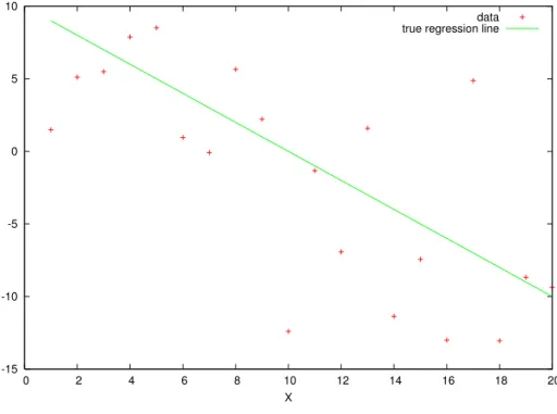
Figure 3.1, obtained by running TypicalData.m shows some data that follows the linear model yt =

β1+β2xt2+t. The green line is the ”true” regression line β1+β2xt2, and the red crosses are the data points (xt2, yt), where t is a random error that has mean zero and is independent of xt2. Exactly how the green line is defined will become clear later. In practice, we only have the data, and we don’t know where the green line lies. We need to gain information about the straight line that best fits the data points.

The ordinary least squares (OLS) estimator is defined as the value that minimizes the sum of the squared errors:

ˆ

β = arg mins(β)

where

s(β) =

n

X

t=1

(yt −x0tβ) 2

(3.2)

= (y−Xβ)0(y−Xβ) = y0y−2y0Xβ +β0X0Xβ

(32)

Figure 3.1: Typical data, Classical Model

-15 -10 -5 0 5 10

0 2 4 6 8 10 12 14 16 18 20

X

(33)

This last expression makes it clear how the OLS estimator is defined: it minimizes the Euclidean dis-tance betweeny and Xβ. The fitted OLS coefficients are those that give the best linear approximation to y using x as basis functions, where ”best” means minimum Euclidean distance. One could think of other estimators based upon other metrics. For example, the minimum absolute distance (MAD) minimizes Pn

t=1|yt −x0tβ|. Later, we will see that which estimator is best in terms of their statistical properties, rather than in terms of the metrics that define them, depends upon the properties of , about which we have as yet made no assumptions.

• To minimize the criterion s(β), find the derivative with respect to β:

Dβs(β) = −2X0y+ 2X0Xβ

Then setting it to zeros gives

Dβs( ˆβ) =−2X0y+ 2X0Xβˆ≡ 0

so

ˆ

β = (X0X)−1X0y.

• To verify that this is a minimum, check the second order sufficient condition:

D_β2s( ˆβ) = 2X0X

(34)

• The fitted values are the vector ˆy = Xβ.ˆ

• The residuals are the vector ˆε= y−Xβˆ

• Note that

y = Xβ+ ε

= Xβˆ+ ˆε

• Also, the first order conditions can be written as

X0y−X0Xβˆ = 0

X0

y−Xβˆ

= 0

X0εˆ = 0

which is to say, the OLS residuals are orthogonal to X. Let’s look at this more carefully.

3.3 Geometric interpretation of least squares estimation

In

X, Y

Space

(35)

Figure 3.2: Example OLS Fit

-15 -10 -5 0 5 10 15

0 2 4 6 8 10 12 14 16 18 20

X

(36)

In Observation Space

If we want to plot in observation space, we’ll need to use only two or three observations, or we’ll encounter some limitations of the blackboard. If we try to use 3, we’ll encounter the limits of my artistic ability, so let’s use two. With only two observations, we can’t have K > 1.

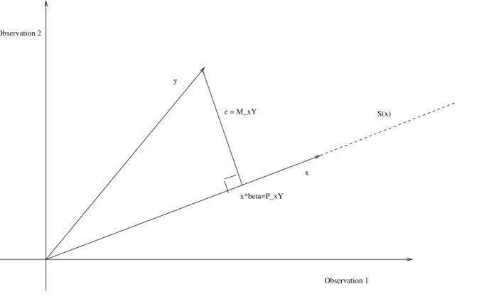
Figure 3.3: The fit in observation space

Observation 2

Observation 1 x

y

S(x)

x*beta=P_xY e = M_xY

• We can decompose y into two components: the orthogonal projection onto the K−dimensional

space spanned by X, Xβ,ˆ and the component that is the orthogonal projection onto the n−K

(37)

• Since ˆβ is chosen to make ˆε as short as possible, ˆε will be orthogonal to the space spanned by

X. Since X is in this space, X0εˆ= 0. Note that the f.o.c. that define the least squares estimator imply that this is so.

Projection Matrices

Xβˆ is the projection of y onto the span of X, or

Xβˆ= X (X0X)−1X0y

Therefore, the matrix that projects y onto the span of X is

PX = X(X0X)−1X0

since

Xβˆ= PXy.

ˆ

ε is the projection of y onto the N −K dimensional space that is orthogonal to the span of X. We have that

ˆ

ε = y −Xβˆ

= y −X(X0X)−1X0y

= hIn −X(X0X)−1X0

(38)

So the matrix that projects y onto the space orthogonal to the span of X is

MX = In−X(X0X)−1X0

= In−PX.

We have

ˆ

ε = MXy.

Therefore

y = PXy +MXy

= Xβˆ+ ˆε.

These two projection matrices decompose the n dimensional vector y into two orthogonal components - the portion that lies in the K dimensional space defined by X, and the portion that lies in the orthogonal n−K dimensional space.

• Note that both PX and MX are symmetric and idempotent.

– A symmetric matrix A is one such that A = A0.

– An idempotent matrix A is one such that A= AA.

(39)

3.4 Influential observations and outliers

The OLS estimator of the ith element of the vector β0 is simply

ˆ

βi =

h

(X0X)−1X0i

i·y

= c0_iy

This is how we define a linear estimator - it’s a linear function of the dependent variable. Since it’s a linear combination of the observations on the dependent variable, where the weights are determined by the observations on the regressors, some observations may have more influence than others.

To investigate this, let et be an n vector of zeros with a 1 in the tth position, i.e., it’s the

tth column of the matrix In. Define

ht = (PX)_tt

= e0_tPXet

so ht is the tth element on the main diagonal of PX. Note that

ht = kPXet k2

so

ht ≤k et k2= 1

So 0< ht < 1. Also,

(40)

So the average of the ht is K/n. The value ht is referred to as the leverage of the observation. If the leverage is much higher than average, the observation has the potential to affect the OLS fit importantly. However, an observation may also be influential due to the value of yt, rather than the weight it is multiplied by, which only depends on the xt’s.

To account for this, consider estimation of β without using the tth observation (designate this estimator as ˆβ(t)). One can show (see Davidson and MacKinnon, pp. 32-5 for proof) that

ˆ

β(t) = ˆβ − 1

1−ht

!

(X0X)−1X_t0εˆt

so the change in the tth observations fitted value is

x0_tβˆ−x0_tβˆ(t) = ht 1−ht

!

ˆ

εt

While an observation may be influential if it doesn’t affect its own fitted value, it certainlyis influential if it does. A fast means of identifying influential observations is to plot

ht

1−ht

ˆ

εt (which I will refer to as the own influence of the observation) as a function of t. Figure 3.4 gives an example plot of data, fit, leverage and influence. The Octave program is InfluentialObservation.m. (note to self when lecturing: load the data ../OLS/influencedata into Gretl and reproduce this). If you re-run the program you will see that the leverage of the last observation (an outlying value of x) is always high, and the influence is sometimes high.

After influential observations are detected, one needs to determinewhy they are influential. Possible causes include:

(41)

Figure 3.4: Detection of influential observations

0 2 4 6 8 10 12 14

0 0.5 1 1.5 2 2.5 3 3.5

(42)

• special economic factors that affect some observations. These would need to be identified and

incorporated in the model. This is the idea behind structural change: the parameters may not be constant across all observations.

• pure randomness may have caused us to sample a low-probability observation.

There exist robust estimation methods that downweight outliers.

3.5 Goodness of fit

The fitted model is

y = Xβˆ+ ˆε

Take the inner product:

y0y = ˆβ0X0Xβˆ+ 2 ˆβ0X0εˆ+ ˆε0εˆ But the middle term of the RHS is zero since X0εˆ= 0, so

(43)

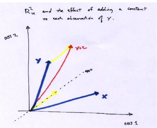
The uncentered R2_u is defined as

R2_u = 1− εˆ

0_ε_ˆ

y0_y

= ˆ

β0X0Xβˆ y0y

= k PXy k 2

k y k2 = cos2(φ),

where φ is the angle between y and the span of X .

• The uncentered R2 changes if we add a constant to y, since this changes φ (see Figure 3.5, the

yellow vector is a constant, since it’s on the 45 degree line in observation space). Another, more common definition measures the contribution of the variables, other than the constant term, to explaining the variation in y. Thus it measures the ability of the model to explain the variation of y about its unconditional sample mean.

Let ι = (1,1, ...,1)0, a n -vector. So

Mι = In −ι(ι0ι)−1ι0

= In −ιι0/n

Mιy just returns the vector of deviations from the mean. In terms of deviations from the mean, equation 3.3 becomes

(44)

(45)

The centered R2_c is defined as

R2_c = 1− εˆ

0_ε_ˆ

y0_M

ιy

= 1− ESS

T SS

where ESS = ˆε0εˆand T SS = y0Mιy=Pnt=1(yt −y¯)2.

Supposing that X contains a column of ones (i.e., there is a constant term),

X0εˆ= 0 ⇒X

t ˆ

εt = 0

so Mιεˆ= ˆε. In this case

y0Mιy = ˆβ0X0MιXβˆ+ ˆε0εˆ So

R2_c = RSS

T SS

where RSS = ˆβ0X0MιXβˆ

• Supposing that a column of ones is in the space spanned by X (PXι = ι), then one can show

that 0 ≤ R2_c ≤1.

3.6 The classical linear regression model

(46)

respect to xj? The linear approximation is

y = β1x1 +β2x2 +...+ βkxk +

The partial derivative is

∂y

∂xj

= βj +

∂

∂xj

Up to now, there’s no guarantee that _∂x∂

j=0. For the β to have an economic meaning, we need to

make additional assumptions. The assumptions that are appropriate to make depend on the data under consideration. We’ll start with the classical linear regression model, which incorporates some assumptions that are clearly not realistic for economic data. This is to be able to explain some concepts with a minimum of confusion and notational clutter. Later we’ll adapt the results to what we can get with more realistic assumptions.

Linearity: the model is a linear function of the parameter vector β0 :

y = β₁0x1 + β20x2 +...+βk0xk + (3.4)

or, using vector notation:

y = x0β0 +

Nonstochastic linearly independent regressors: X is a fixed matrix of constants, it has rank

K equal to its number of columns, and

lim 1

nX

0_X ₌ _Q

(47)

whereQX is a finite positive definite matrix. This is needed to be able to identify the individual effects of the explanatory variables.

Independently and identically distributed errors:

∼IID(0, σ2In) (3.6)

ε is jointly distributed IID. This implies the following two properties:

Homoscedastic errors:

V(εt) = σ02,∀t (3.7)

Nonautocorrelated errors:

E(εts) = 0,∀t 6= s (3.8)

Optionally, we will sometimes assume that the errors are normally distributed.

Normally distributed errors:

∼ N(0, σ2In) (3.9)

3.7 Small sample statistical properties of the least squares

estimator

(48)

Unbiasedness

We have ˆβ = (X0X)−1X0y. By linearity,

ˆ

β = (X0X)−1X0(Xβ + ε)

= β + (X0X)−1X0ε

By 3.5 and 3.6

E(X0X)−1X0ε = E(X0X)−1X0ε

= (X0X)−1X0Eε

= 0

so the OLS estimator is unbiased under the assumptions of the classical model.

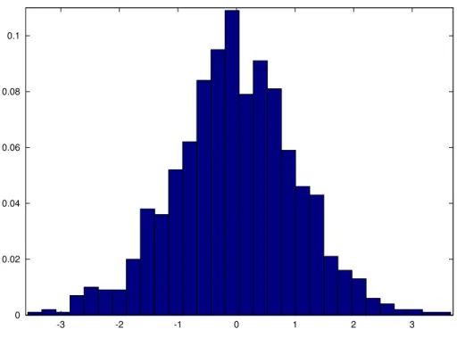
Figure 3.6 shows the results of a small Monte Carlo experiment where the OLS estimator was calculated for 10000 samples from the classical model with y = 1 + 2x+ε, where n = 20, σ_ε2 = 9, and

x is fixed across samples. We can see that the β2 appears to be estimated without bias. The program that generates the plot is Unbiased.m , if you would like to experiment with this.

With time series data, the OLS estimator will often be biased. Figure 3.7 shows the results of a small Monte Carlo experiment where the OLS estimator was calculated for 1000 samples from the AR(1) model with yt = 0 + 0.9yt−1 +εt, where n = 20 and σε2 = 1. In this case, assumption 3.5 does not hold: the regressors are stochastic. We can see that the bias in the estimation of β2 is about -0.2.

(49)

Figure 3.6: Unbiasedness of OLS under classical assumptions

0 0.02 0.04 0.06 0.08 0.1

(50)

Figure 3.7: Biasedness of OLS when an assumption fails

0 0.02 0.04 0.06 0.08 0.1 0.12

(51)

Normality

With the linearity assumption, we have ˆβ = β + (X0X)−1X0ε. This is a linear function of ε. Adding the assumption of normality (3.9, which implies strong exogeneity), then

ˆ

β ∼ N β,(X0X)−1σ2₀

since a linear function of a normal random vector is also normally distributed. In Figure 3.6 you can see that the estimator appears to be normally distributed. It in fact is normally distributed, since the DGP (see the Octave program) has normal errors. Even when the data may be taken to be IID, the assumption of normality is often questionable or simply untenable. For example, if the dependent variable is the number of automobile trips per week, it is a count variable with a discrete distribution, and is thus not normally distributed. Many variables in economics can take on only nonnegative values, which, strictly speaking, rules out normality.2

The variance of the OLS estimator and the Gauss-Markov theorem

Now let’s make all the classical assumptions except the assumption of normality. We have ˆβ =

β+ (X0X)−1X0ε and we know that E( ˆβ) =β. So

V ar( ˆβ) = E

(

ˆ

β −β βˆ−β

0)

= En(X0X)−1X0εε0X(X0X)−1o = (X0X)−1σ₀2

2_{Normality may be a good model nonetheless, as long as the probability of a negative value occuring is negligable under the model. This}

(52)

The OLS estimator is a linear estimator, which means that it is a linear function of the dependent variable, y.

ˆ

β = h(X0X)−1X0iy

= Cy

where C is a function of the explanatory variables only, not the dependent variable. It is also unbiased under the present assumptions, as we proved above. One could consider other weights W that are a function of X that define some other linear estimator. We’ll still insist upon unbiasedness. Consider

˜

β = W y, where W = W(X) is some k×n matrix function of X. Note that since W is a function of

X, it is nonstochastic, too. If the estimator is unbiased, then we must have W X = IK:

E(W y) = E(W Xβ0 +W ε)

= W Xβ0

= β0

⇒

W X = IK

The variance of ˜β is

V( ˜β) = W W0σ₀2.

Define

(53)

so

W = D + (X0X)−1X0

Since W X = IK, DX = 0, so

V( ˜β) = D + (X0X)−1X0 D + (X0X)−1X00σ₀2

=

DD0+ (X0X)−1

σ₀2

So

V( ˜β) ≥V( ˆβ)

The inequality is a shorthand means of expressing, more formally, that V( ˜β) − V( ˆβ) is a positive semi-definite matrix. This is a proof of the Gauss-Markov Theorem. The OLS estimator is the ”best linear unbiased estimator” (BLUE).

• It is worth emphasizing again that we have not used the normality assumption in any way to

prove the Gauss-Markov theorem, so it is valid if the errors are not normally distributed, as long as the other assumptions hold.

(54)

Figure 3.8: Gauss-Markov Result: The OLS estimator

are more narrow.

We have that E( ˆβ) =β and V ar( ˆβ) =X0X−1σ₀2, but we still need to estimate the variance of ,

σ2₀, in order to have an idea of the precision of the estimates of β. A commonly used estimator of σ₀2 is

c

σ₀2 = 1

n−Kεˆ

0_ˆ

ε

(55)

(56)

c

σ₀2 = 1

n−Kεˆ

0_ε_ˆ

= 1

n−Kε

0

M ε

E(σc2

0) =

1

n−KE(T rε

0_{M ε}₎

= 1

n−KE(T rM εε

0₎

= 1

n−KT rE(M εε

0₎

= 1

n−Kσ

2 0T rM

= 1

n−Kσ

2

0 (n−k) = σ2₀

where we use the fact that T r(AB) = T r(BA) when both products are conformable. Thus, this estimator is also unbiased under these assumptions.

3.8 Example: The Nerlove model

Theoretical background

(57)

min_x w0x

subject to the restriction

f(x) = q.

The solution is the vector of factor demands x(w, q). The cost function is obtained by substituting the factor demands into the criterion function:

Cw, q) =w0x(w, q).

• Monotonicity Increasing factor prices cannot decrease cost, so

∂C(w, q)

∂w ≥0

Remember that these derivatives give the conditional factor demands (Shephard’s Lemma).

• Homogeneity The cost function is homogeneous of degree 1 in input prices: C(tw, q) = tC(w, q)

where t is a scalar constant. This is because the factor demands are homogeneous of degree zero in factor prices - they only depend upon relative prices.

• Returns to scale The returns to scale parameter γ is defined as the inverse of the elasticity of

cost with respect to output:

γ =





∂C(w, q)

∂q

q

C(w, q)





(58)

Constant returns to scale is the case where increasing production q implies that cost increases in the proportion 1:1. If this is the case, then γ = 1.

Cobb-Douglas functional form

The Cobb-Douglas functional form is linear in the logarithms of the regressors and the dependent variable. For a cost function, if there are g factors, the Cobb-Douglas cost function has the form

C = Awβ1

1 ...wgβgq βq_eε

What is the elasticity of C with respect to wj?

eC_w_j =



 ∂C

∂WJ





wj

C !

= βjAw β1

1 .w βj−1

j ..w βg

g q

βq_eε wj

Awβ1

1 ...w βg

g qβqeε = βj

This is one of the reasons the Cobb-Douglas form is popular - the coefficients are easy to interpret, since they are the elasticities of the dependent variable with respect to the explanatory variable. Not that in this case,

eC_w_j =



 ∂C

∂WJ





wj

C !

= xj(w, q)

wj

C

(59)

the cost share of the jth input. So with a Cobb-Douglas cost function, βj = sj(w, q). The cost shares are constants.

Note that after a logarithmic transformation we obtain

lnC = α+β1lnw1 +...+βglnwg +βqlnq +

where α = lnA . So we see that the transformed model is linear in the logs of the data. One can verify that the property of HOD1 implies that

g

X

i=1

βg = 1

In other words, the cost shares add up to 1.

The hypothesis that the technology exhibits CRTS implies that

γ = 1

βq = 1

so βq = 1. Likewise, monotonicity implies that the coefficients βi ≥ 0, i = 1, ..., g.

The Nerlove data and OLS

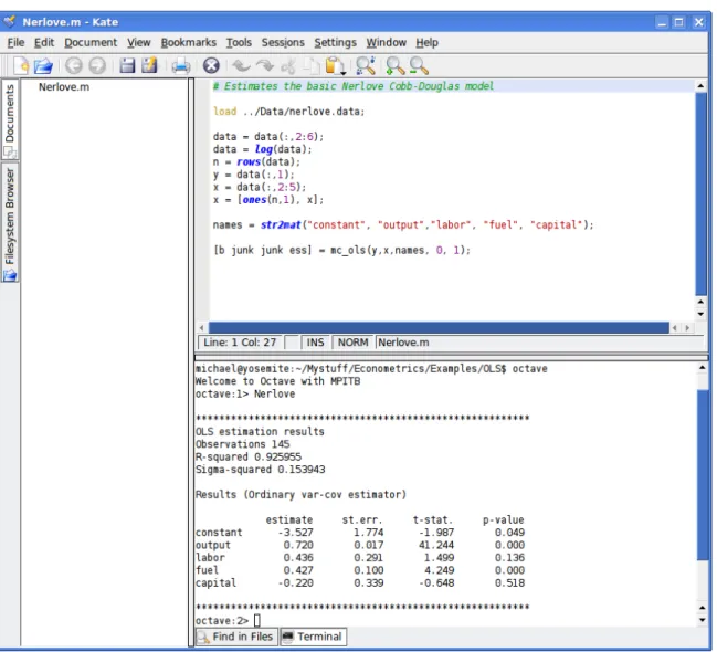
The file nerlove.data contains data on 145 electric utility companies’ cost of production, output and input prices. The data are for the U.S., and were collected by M. Nerlove. The observations are by row, and the columns are COMPANY, COST (C), OUTPUT (Q), PRICE OF LABOR (PL),

(60)

level (the third column).

We will estimate the Cobb-Douglas model

lnC = β1 +β2lnQ+β3lnPL +β4lnPF +β5lnPK + (3.10)

using OLS. To do this yourself, you need the data file mentioned above, as well as Nerlove.m (the estimation program), and the library of Octave functions mentioned in the introduction to Octave that forms section 24 of this document.3

The results are

********************************************************* OLS estimation results

Observations 145 R-squared 0.925955 Sigma-squared 0.153943

Results (Ordinary var-cov estimator)

estimate st.err. t-stat. p-value

constant -3.527 1.774 -1.987 0.049

output 0.720 0.017 41.244 0.000

labor 0.436 0.291 1.499 0.136

fuel 0.427 0.100 4.249 0.000

capital -0.220 0.339 -0.648 0.518

*********************************************************

(61)

• Do the theoretical restrictions hold?

• Does the model fit well?

• What do you think about RTS?

While we will most often use Octave programs as examples in this document, since following the programming statements is a useful way of learning how theory is put into practice, you may be interested in a more ”user-friendly” environment for doing econometrics. I heartily recommend Gretl, the Gnu Regression, Econometrics, and Time-Series Library. This is an easy to use program, available in English, French, and Spanish, and it comes with a lot of data ready to use. It even has an option to save output as LA_{TEX fragments, so that I can just include the results into this document, no muss,} no fuss. Here is the Nerlove data in the form of a GRETL data set: nerlove.gdt . Here the results of the Nerlove model from GRETL:

Model 2: OLS estimates using the 145 observations 1–145 Dependent variable: l_cost

Variable Coefficient Std. Error t-statistic p-value

const −3.5265 1.77437 −1.9875 0.0488

l_output 0.720394 0.0174664 41.2445 0.0000

l_labor 0.436341 0.291048 1.4992 0.1361

l_fuel 0.426517 0.100369 4.2495 0.0000

(62)

Mean of dependent variable 1.72466 S.D. of dependent variable 1.42172 Sum of squared residuals 21.5520 Standard error of residuals (ˆσ) 0.392356 Unadjusted R2 0.925955 Adjusted ¯R2 0.923840

F(4,140) 437.686

Akaike information criterion 145.084 Schwarz Bayesian criterion 159.967

Fortunately, Gretl and my OLS program agree upon the results. Gretl is included in the bootable CD mentioned in the introduction. I recommend using GRETL to repeat the examples that are done using Octave.

The previous properties hold for finite sample sizes. Before considering the asymptotic properties of the OLS estimator it is useful to review the MLE estimator, since under the assumption of normal errors the two estimators coincide.

3.9 Exercises

1. Prove that the split sample estimator used to generate figure 3.9 is unbiased.

2. Calculate the OLS estimates of the Nerlove model using Octave and GRETL, and provide print-outs of the results. Interpret the results.

(63)

Nerlove model. Discuss.

4. Using GRETL, examine the residuals after OLS estimation and tell me whether or not you believe that the assumption of independent identically distributed normal errors is warranted. No need to do formal tests, just look at the plots. Print out any that you think are relevant, and interpret them.

5. For a random vector X ∼ N(µx,Σ), what is the distribution of AX + b, where A and b are conformable matrices of constants?

6. Using Octave, write a little program that verifies that T r(AB) = T r(BA) for A and B 4x4 matrices of random numbers. Note: there is an Octave function trace.

(64)

Chapter 4

Asymptotic properties of the least

squares estimator

The OLS estimator under the classical assumptions is BLUE1, for all sample sizes. Now let’s see what happens when the sample size tends to infinity.

1_BLUE _≡_{best linear unbiased estimator if I haven’t defined it before}

(65)

4.1 Consistency

ˆ

β = (X0X)−1X0y

= (X0X)−1X0(Xβ + ε) = β0 + (X0X)−1X0ε = β0 +





X0X

n 



−1

X0ε

n

Consider the last two terms. By assumption limn→∞

_X0_X

n

= QX ⇒ limn→∞

_X0_X

n

−1

= Q−_X1, since the inverse of a nonsingular matrix is a continuous function of the elements of the matrix. Considering X0ε

n ,

X0ε

n = 1 n n X t=1

xtεt

Each xtεt has expectation zero, so

E 



X0ε

n 

 = 0

The variance of each term is

V (xtt) = xtx0tσ

(66)

As long as these are finite, and given a technical condition2, the Kolmogorov SLLN applies, so

1

n

X

t=1

xtεt a.s. → 0.

This implies that

ˆ

β a.s.→ β0.

This is the property of strong consistency: the estimator converges in almost surely to the true value.

• The consistency proof does not use the normality assumption.

• Remember that almost sure convergence implies convergence in probability.

4.2 Asymptotic normality

We’ve seen that the OLS estimator is normally distributed under the assumption of normal errors. If the error distribution is unknown, we of course don’t know the distribution of the estimator. However, we can get asymptotic results. Assuming the distribution of ε is unknown, but the the other classical assumptions hold:

2_{For application of LLN’s and CLT’s, of which there are very many to choose from, I’m going to avoid the technicalities. Basically, as long}

(67)

ˆ

β = β0 + (X0X)−1X0ε

ˆ

β −β0 = (X0X)−1X0ε

√

n

ˆ

β −β0

=





X0X

n 



−1

X0ε

√

n

• Now as before, X_n0X−1 →Q−_X1.

• Considering X√0ε

n, the limit of the variance is

lim n→∞V





X0ε

√

n 

 = lim

n→∞E





X00X

n 



= σ₀2QX

The mean is of course zero. To get asymptotic normality, we need to apply a CLT. We assume one (for instance, the Lindeberg-Feller CLT) holds, so

X0ε

√

n

d

→ N0, σ₀2QX

Therefore, √ n ˆ

β −β0

d

→ N 0, σ₀2Q−_X1 (4.1)

• In summary, the OLS estimator is normally distributed in small and large samples ifε is normally

(68)

CLT can be applied.

4.3 Asymptotic efficiency

The least squares objective function is

s(β) =

n

X

t=1

(yt −x0tβ) 2

Supposing that ε is normally distributed, the model is

y = Xβ0 +ε,

ε ∼ N(0, σ₀2In), so

f(ε) =

n

Y

t=1 1 √

2πσ2 exp



−

ε2_t

2σ2





The joint density fory can be constructed using a change of variables. We have ε= y−Xβ, so _∂y∂ε0 = In and |∂ε

∂y0| = 1, so

f(y) =

n

Y

t=1 1 √

2πσ2 exp



−

(yt −x0tβ)2 2σ2



.

Taking logs,

lnL(β, σ) = −nln√2π −nlnσ− n

X

t=1

(yt −x0tβ) 2

(69)

Maximizing this function with respect to β and σ gives what is known as the maximum likelihood (ML) estimator. It turns out that ML estimators are asymptotically efficient, a concept that will be explained in detail later. It’s clear that the first order conditions for the MLE ofβ0 are the same as the first order conditions that define the OLS estimator (up to multiplication by a constant), so the OLS estimator of β is also the ML estimator. The estimators are the same, under the present assumptions. Therefore, their properties are the same. In particular, under the classical assumptions with normality, the OLS estimator βˆ is asymptotically efficient. Note that one needs to make an assumption about the distribution of the errors to compute the ML estimator. If the errors had a distribution other than the normal, then the OLS estimator and the ML estimator would not coincide.

As we’ll see later, it will be possible to use (iterated) linear estimation methods and still achieve asymptotic efficiency even if the assumption that V ar(ε) 6= σ2In, as long as ε is still normally dis-tributed. This is not the case if ε is nonnormal. In general with nonnormal errors it will be necessary to use nonlinear estimation methods to achieve asymptotically efficient estimation.

4.4 Exercises

1. Write an Octave program that generates a histogram forRMonte Carlo replications of√n

ˆ

βj −βj

,

(70)

Chapter 5

Restrictions and hypothesis tests

5.1 Exact linear restrictions

In many cases, economic theory suggests restrictions on the parameters of a model. For example, a demand function is supposed to be homogeneous of degree zero in prices and income. If we have a Cobb-Douglas (log-linear) model,

lnq = β0 + β1lnp1 +β2lnp2 +β3lnm+ε,

then we need that

k0lnq = β0 +β1lnkp1 +β2lnkp2 + β3lnkm+ ε,

(71)

so

β1lnp1 +β2lnp2 +β3lnm = β1lnkp1 +β2lnkp2 +β3lnkm

= (lnk) (β1 + β2 +β3) +β1lnp1 + β2lnp2 +β3lnm.

The only way to guarantee this for arbitrary k is to set

β1 + β2 + β3 = 0,

which is a parameter restriction. In particular, this is a linear equality restriction, which is probably the most commonly encountered case.

Imposition

The general formulation of linear equality restrictions is the model

y = Xβ +ε

Rβ = r

where R is a Q×K matrix, Q < K and r is a Q×1 vector of constants.

• We assume R is of rank Q, so that there are no redundant restrictions.

(72)

Let’s consider how to estimate β subject to the restrictions Rβ = r. The most obvious approach is to set up the Lagrangean

min

β s(β) = 1

n(y −Xβ)

0

(y −Xβ) + 2λ0(Rβ −r).

The Lagrange multipliers are scaled by 2, which makes things less messy. The fonc are

Dβs( ˆβ,λˆ) = −2X0y + 2X0XβˆR + 2R0ˆλ ≡ 0

Dλs( ˆβ,λˆ) = RβˆR −r ≡0,

which can be written as



 

X0X R0

R 0       ˆ βR ˆ λ   =   

X0y

r   . We get    ˆ βR ˆ λ    =   

X0X R0

R 0



 

−1  

X0y

r 

 .

(73)

Note that



 

(X0X)−1 0 −R(X0X)−1 IQ

     

X0X R0

R 0





 ≡ AB

=



 

IK (X0X)−1R0

0 −R(X0X)−1R0    ≡   

IK (X0X)

−1

R0

0 −P

   ≡ C, and   

IK (X0X)−1R0P−1

0 −P−1

     

IK (X0X)−1R0

0 −P





 ≡ DC

= IK+Q,

so

DAB = IK+Q

DA = B−1

B−1 =



 

IK (X0X)−1R0P−1

0 −P−1

     

(X0X)−1 0 −R(X0X)−1 IQ

   =   

(X0X)−1 −(X0X)−1R0P−1R(X0X)−1 (X0X)−1R0P−1

P−1R(X0X)−1 −P−1



(74)

If you weren’t curious about that, please start paying attention again. Also, note that we have made the definition P = R(X0X)−1R0)

   ˆ βR ˆ λ    =   

(X0X)−1 −(X0X)−1R0P−1R(X0X)−1 (X0X)−1R0P−1

P−1R(X0X)−1 −P−1

     

X0y

r    =     ˆ

β −(X0X)−1R0P−1

Rβˆ−r

P−1

Rβˆ−r

    =   

(IK −(X0X)−1R0P−1R)

P−1R

   ˆ β +   

(X0X)−1R0P−1r

−P−1r



 

The fact that ˆβR and ˆλ are linear functions of ˆβ makes it easy to determine their distributions, since the distribution of ˆβ is already known. Recall that for x a random vector, and for A and b a matrix and vector of constants, respectively, V ar(Ax+b) = AV ar(x)A0.

Though this is the obvious way to go about finding the restricted estimator, an easier way, if the number of restrictions is small, is to impose them by substitution. Write

y = X1β1 + X2β2 +ε

R1 R2

   β1 β2  

 = r

where R1 is Q×Qnonsingular. Supposing the Q restrictions are linearly independent, one can always make R1 nonsingular by reorganizing the columns of X. Then

Econometría Michael Creel (2014)

Econometrics

Contents

List of Figures

List of Tables

Chapter 1

About this document

1.1

Prerequisites

1.2

Contents

1.3

Licenses

1.4

Obtaining the materials

1.5

An easy way run the examples

Chapter 2

Introduction: Economic and

econometric models

Chapter 3

Ordinary Least Squares

3.1

The Linear Model

3.2

Estimation by least squares

3.3

Geometric interpretation of least squares estimation

In

X, Y

Space

In Observation Space

Projection Matrices

3.4

Influential observations and outliers

3.5

Goodness of fit

3.6

The classical linear regression model

3.7

Small sample statistical properties of the least squares

estimator

Unbiasedness

Normality

The variance of the OLS estimator and the Gauss-Markov theorem

3.8

Example: The Nerlove model

Theoretical background

Cobb-Douglas functional form

The Nerlove data and OLS

3.9

Exercises

Chapter 4

Asymptotic properties of the least

squares estimator

4.1

Consistency

4.2

Asymptotic normality

4.3

Asymptotic efficiency

4.4

Exercises

Chapter 5

Restrictions and hypothesis tests

5.1

Exact linear restrictions

Imposition