A diversity of beta diversities: straightening up a concept gone
awry. Part 1. Defining beta diversity as a function of alpha and
gamma diversity
Hanna Tuomisto
H. Tuomisto ([email protected]), Dept of Biology, FI-20014 Univ. of Turku, Finland.
The termbeta diversityhas been used to refer to a wide variety of phenomena. Although all of these encompass some kind of compositional heterogeneity between places, many are not related to each other in any predictable way. The present two-part review aims to put the different phenomena that have been called beta diversity into a common conceptual framework, and to explain what each of them measures. In this first part, the focus is on defining a beta component of diversity. This involves deciding what diversity is and how the observed total or gamma diversity (g) is partitioned into alpha (a) and beta (b) components. Several different definitions of ‘‘beta diversity’’ that result from these decisions have been used in the ecological literature.True beta diversityis obtained when the total effective number of species in a dataset (true gamma diversityg) is multiplicatively partitioned into the effective number of species per compositionally distinct virtual sampling unit (true alpha diversityad) and the effective number of such compositional units (bMdg/ad). All true
diversities quantify the effective number of types of entities. Because the other variants of ‘‘beta diversity’’ that have been used by ecologists quantify other phenomena, an alternative nomenclature is proposed here for the seven most popular beta components: regional-to-local diversity ratio, two-way diversity ratio, absolute effective species turnover (regional diversity excess), Whittaker’s effective species turnover, proportional effective species turnover, regional entropy excess and regional variance excess. In the second part of the review, the focus will be on how to quantify these phenomena in practice. This involves deciding how the sampling units that contribute to total diversity are selected, and whether the entity that is quantified is all of ‘‘beta diversity’’, a specific part of ‘‘beta diversity’’, the rate of change in ‘‘beta diversity’’ in relation to a given external factor, or something else.
In a seminal paper, Whittaker (1960, p. 320) defined beta diversity as ‘‘The extent of change in community composition, or degree of community differentiation, in relation to a complex-gradient of environment, or a pattern of environments’’. He then proceeded to quantify beta diversity in different ways. His first two cases concerned Jaccard index (example 1) and percentage similarity (example 2) values between vegetation samples differing in geological formation and/or local moisture conditions. His third example quantified beta diversity as the ratio of gamma diversity (diversity in a set of sampling units) to alpha diversity (average diversity within sampling units) within each geological formation. His fourth example quantified beta diversity as the number of half-change units, the half-change unit being the distance along a transect by which similarity between two sampling units decreases to one-half of the value estimated for similar environments.
Obviously, Whittaker (1960) did not have an exact definition of beta diversity in mind, but used the term in a rather vague sense to refer to compositional heterogeneity among places. His verbal definition of beta diversity was
broad, and each new example added a new phenomenon to it. All of the quantitative definitions are ratios that can be interpreted as unitless, but in fact their measurement units are species/species (example 1), (% abundance)/(% abun-dance) (example 2), (unit of diversity index)/(unit of diversity index) (example 3) and (unit of external gradi-ent)/(unit of external gradient) (example 4). Under these definitions, beta diversity can be calculated for sampling units representing different habitat classes (examples 1 and 2), the same habitat class (example 3), or a gradient that has not been divided into habitat classes (example 4). Beta diversity may be explicitly dependent on a specified external gradient (distance along a transect in example 4) or not (examples 1, 2 and 3). Either species presence-absence data (examples 1 and 4) or quantitative abundance data (examples 2, 3 and 4) can be used in different mathematical formulae.
Whittaker (1960) introduced the term beta diversity (b) together with alpha diversity (a) and gamma diversity (g). Bothaandgrepresent species diversity, butais the mean species diversity at the local, within-site or within-habitat scale, whereasgis the total species diversity at the regional Ecography 33: 222, 2010 doi: 10.1111/j.1600-0587.2009.05880.x
#2010 The Author. Journal compilation#2010 Ecography
or landscape scale. Cody (1975) redefinedbeta diversityas the rate of compositional turnover along a habitat gradient within one geographical region, andgamma diversityas the rate of compositional turnover with geographical distance within one habitat. Bratton (1975) also used the term beta diversity to refer to the rate of species turnover along a gradient. Whittaker (1977) accepted this expansion ofbeta diversity, which then became the ‘‘extent or rate of change in composition’’. To account for different spatial scales, Whittaker (1977) proposed a hierarchical nomenclature in which alpha diversity refers to within-habitat diversity, beta diversity to among-habitat differentiation in a landscape, gamma diversity to total within-landscape diversity, delta diversityto among-landscape differentiation in a region, and epsilon diversityto total within-region diversity.
No wonder, therefore, that researchers have had a hard time agreeing on which quantitative interpretation of beta diversity is the correct one. Sources of contention include how beta diversity should be calculated, whether it should be measured within habitats or between habitats, and what spatial scales are appropriate. Several attempts have been made to tie alpha and gamma diversity to specific spatial scales (reviewed in Whittaker et al. 2001 and Magurran 2004), but little consensus has emerged on this point. However, usually researchers are interested in habitats and regions so extensive that full species inventories are a practical impossiblity, so that obtaining accurate estimates of alpha and gamma diversity is a major concern (Colwell and Coddington 1994, Plotkin and Muller-Landau 2002, Chao et al. 2006).
Here I do not wish to dwell on how to delimit local, regional or habitat in practice, or on issues of data representativeness. Although these are important questions, the logical definition of the phenomenon that is to be measured needs to be established before it is useful to discuss practical sampling problems. Therefore I will treat all diversity components as properties of a dataset: once it has been decided which data points form the dataset of interest, all diversity components can be exactly quantified for that dataset. In this context, spatial scales are arbitrary and can be selected freely. The data need to come from discrete sampling units embedded in a study region, but whether lag (distance between neighboring sampling units) is small or large is irrelevant. The extent of the study corresponds to the size of the study region and the grain to the size of the sampling unit. Delta and epsilon diversities become unnecessary, because they simply refer to beta and gamma diversity, respectively, in a study system with large grain and extent. Grain and extent affect the numerical values of the diversity components, and lag needs to be taken into account when extrapolating results from an existing dataset to uninventoried areas. These issues will be discussed in the second part of the present review (Tuomisto 2010), once the basic concepts have been defined.
Defining beta diversity is the main topic of the present paper. All variants of the umbrella concept encompass some kind of heterogeneity, differentiation or complemen-tarity, but they actually refer to quite different phenomena. Some of these phenomena vary independently of each other among datasets, and ‘‘beta diversity’’ values based on
different variants may therefore not be correlated. The situation is similar to that for the umbrella conceptsize. If we did not have separate words for weight, length, height, area and volume, discussions on size would become very confusing. The situation would become even worse if the term size were not only used for both weight and height, but also for growth rate. For example, consider animal A whose size is 100 cm, and animal B whose size is 10 kg. Which animal is bigger? It is impossible to say, because the given values are not commensurate. If the weight of A is revealed to be 5 kg, we know that B is heavier than A. But finding out that the size of B is 100 allows no conclusions, because we do not know if the unit of measurement was inches, meters, grams, pounds or something else. Furthermore, different aspects of size may rank animals differently; a snake that is larger than an elephant by the body length criterion is probably smaller by the body height or body weight criterion. If ranking is done using growth rate as the size criterion, it may be found that the younger the animal, the ‘‘larger’’ it is, and that in old animals ‘‘size’’ can even obtain a negative value.
Comparing measurements based on different variants of the umbrella concept is equally useless in the case of ‘‘beta diversity’’. Some variants of ‘‘beta diversity’’ are ratios in which the measurement units cancel out, whereas the measurement units in others can be, for example, virtual sampling units, species, (virtual species)1, bits, species per unit sampling effort, km1, species per km or species per unit habitat gradient. Because all variants of ‘‘beta diversity’’ are both multivariate and abstract, such crucial differences among them are much more difficult to spot than in the case of size. Consequently, the beta diversity literature is replete with studies that commit errors analogous to drawing conclusions on height on the basis of results on weight, or to comparing how two studies ranked different animal species without noticing that one study had measured body length whereas the other had measured the rate at which the animals’ weight increased over time.
Many authors have commented on the confusion around the concept of beta diversity (Gray 2000, Vellend 2001, Koleff et al. 2003a, b, Novotny and Weiblen 2005). The most thorough review to date seems to be that by Jurasinski et al. (2009), who classified several beta diversity concepts into two categories. My aim in the present review is to explain what those and many other variants of ‘‘beta diversity’’ actually mean, and to put them into a common conceptual framework. It is crucial to use a metric that appropriately represents the phenomenon of interest, and knowledge about the logical relationships among alterna-tives can help in making that choice.
‘‘beta diversity’’ in relation to some external factor, or someting else. Each approach leads to quantifying a different phenomenon, but all have been called beta diversity. To facilitate more accurate communication in the future, other names will here be proposed for all variants other than true beta diversity.
The starting point: what is diversity?
Diversity in relation to a single classification
In order to measure diversity in a dataset of interest, the entities of which it is composed (such as individuals) need to be classified into types (such as species). Let us call the classification of individuals (or other appropriate units of abundance) into species the g-classification. Total diversity in relation to the g-classification isgamma diversity(g), or total species diversity. The simplest measure of diversity is the number of types recognised, in this case species richness S. This equals the number of columns in a sites by species table (Table 1). In the present paper, S itself is used as a unitless number; the annotation S sp will be used, when necessary, to make the measurement unit (species) explicit. The number of types has the important doubling property, which can be understood by a thought experiment (Hill 1973, Wilson and Shmida 1984). Imagine that each column in Table 1 is split into two columns, and each proportional abundance value of the original species is evenly divided between the two new species. Intuitively, the species diversity of the dataset has thereby doubled, and so has its species richness.
If all species are equally abundant, each of their proportional abundances (column totals in Table 1) equal 1/S. Mean proportional abundance then also equals 1/S. When proportional abundances vary, their mean can be expressed 1/SE. The inverse of this mean,SE, is the number
of equally-abundant virtual species (effective species) in the
dataset, also known as the effective number of species or species diversity (MacArthur 1965, Hill 1973, Jost 2006). The measurement unit becomes spE, where subscript ‘‘E’’
refers to effective. True species diversity hence quantifies how many effective species the dataset represents, given the mean proportional abundance of the actual species. In fact, diversity in general can be defined in this way: the true diversity of the types of entities of interest is the inverse of the mean of their proportional abundances.
A mean can be calculated in different ways, with some kinds of mean giving more weight to small values and others to large values. The weighted generalised mean with exponent q1 allows a balance to be chosen that is appropriate for the questions at hand (Hill 1973):
¯
pi
q1
ffiffiffiffiffiffiffiffiffiffiffiffiffiffiffiffiffiffiffiffiffi XS
i1
pip q1
i v u u
t XS
i1
pqi 1=(q1)
Herepiis the proportional abundance of theith species (see Table 1 for annotation of proportional abundances). This expression becomes the harmonic mean when q0, the geometric mean in the limit as q approaches unity, the arithmetic mean when q2 and the maximum value in the limit asqapproches infinity. Each species is nominally weighted by the proportion of the data it contributes to the dataset, i.e. bypiitself, but the effective species weights also depend on q. Whenq1, the effective weights equal the nominal weights, and each speciesiaffects the mean exactly in proportion to pi. Asq is increased, the most abundant species gain more effective weight and the mean gradually approaches the largestpivalue in the dataset no matter how many species the dataset contains. As q is decreased, the least abundant species gain more effective weight, such that at q0 all effective weights are the same and the mean equals 1/S no matter how unequal the pi values. When qB0, the least abundant species would get more effective weight than the most abundant species, and the effective number of species would exceed the actual number of
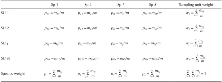
Table 1. A raw data table indicating how themobserved entities of interest have been classified into species according to theg-classification (columns) and into sampling units (SU) according to thev-classification (rows). The absolute abundance of speciesiin sampling unitjis annotatedmij, and each cell value in the table (pij) gives this as a proportion of the total abundancemof all species in the dataset. Absolute
abundance can be quantified using any measure that is appropriate for the questions at hand, for example number of individuals, surface area or biomass. The row totals show the proportion of the total abundance contributed by sampling unitj, i.e. the weight of sampling unitjin the dataset. The column totals show the proportion of the total abundance contributed by speciesi, i.e. the weight of speciesiin the dataset. The proportional abundance of speciesiwithin the limits of sampling unitjispi½jpij/wjfrom which follows thatpijwjpi½j.
Sp 1 Sp 2 Spi SpS Sampling unit weight
SU 1 p11m11/m p21m21/m pi1mi1/m pS1mS1/m /w1a
S i1
mi1
m
SU 2 p12m12/m p22m22/m pi2mi2/m pS2mS2/m /w2a
S i1
mi2
m
SUj p1jm1j/m p2jm2j/m pijmij/m pSjmSj/m /wja
S i1
mij
m
SUN p1Nm1N/m p2Nm2N/m piNmiN/m pSNmSN/m /wNa
S i1
miN
m
Species weight /p1a
N j1
m1j
m /p2a
N j1
m2j
m /pia
N j1
mij
m /pSa
N j1
mSj
m /a
N j1 a
S i1
mij
species observed, so q must logically be restricted to nonnegative values.
True diversity is the inverse ofp¯iand equals (Hill 1973)
qD
gp¯
1
i
XS
i1
piq 1=(1q)
(ql
g)
1=(1q)
where subscript ‘‘g’’ indicates that the calculations are based on theg-classification (see Table 2 for annotation of derived variables). When either q0 or all pi are equal,
thenSESand henceqDgS spE. Otherwise,SEBSand
therefore qDgBS spE. The difference between the actual
and effective number of species increases as the value of qand/or the inequality among thepivalues increase.
The term ql
ga
S i1p
q ip¯
q1
i ;known as thebasic sum, is important because most of the popular species diversity indices can be derived from it (Hill 1973, Keylock 2005). For example, 0lg equals species richness, 2lg Simpson’s
index, 1/2lgthe inverse Simpson index, 12lgthe
Gini-Simpson index and lg the Berger-Parker index. The
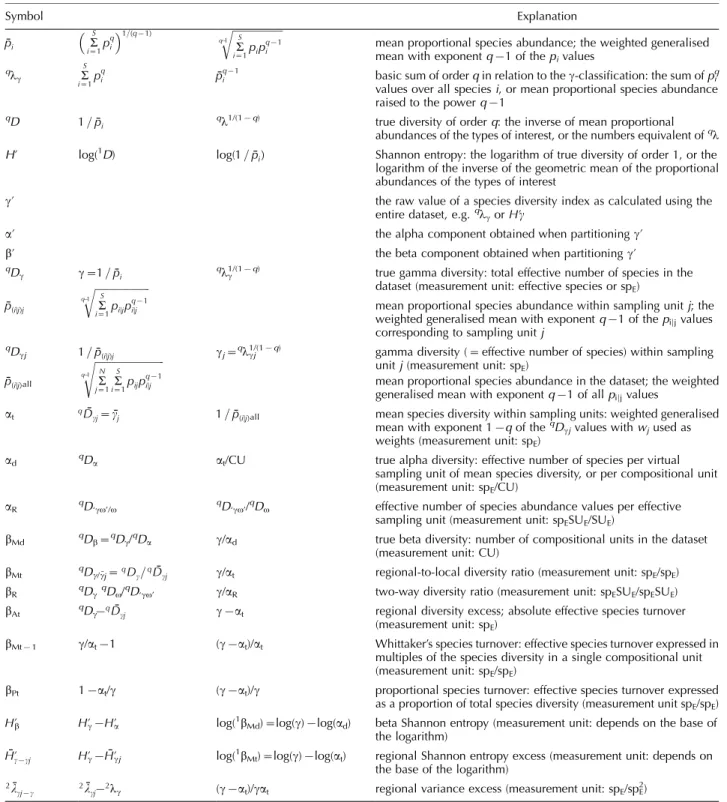
Table 2. Summary of the annotation used for the variables derived from species proportional abundances. Synonymous expressions are listed on the same line. Annotation related to the proportional abundances themselves is explained in Table 1.
Symbol Explanation
/p¯i /
aS
i1p
q i
1=(q1)
/
ffiffiffiffiffiffiffiffiffiffiffiffiffiffiffiffiffiffiffiffi
aS
i1pip
q1
i
q1
r
mean proportional species abundance; the weighted generalised mean with exponentq1 of thepivalues
ql
g /a
S i1p
q
i /p¯q
1
i basic sum of orderqin relation to theg-classification: the sum ofpiq
values over all speciesi, or mean proportional species abundance raised to the powerq1
qD
/1=p¯i ql1/(1q) true diversity of orderq: the inverse of mean proportional abundances of the types of interest, or the numbers equivalent ofql
H? log(1D) log(
/1=p¯i) Shannon entropy: the logarithm of true diversity of order 1, or the logarithm of the inverse of the geometric mean of the proportional abundances of the types of interest
g? the raw value of a species diversity index as calculated using the
entire dataset, e.g.ql
gorH?g
a? the alpha component obtained when partitioningg?
b? the beta component obtained when partitioningg?
qD
g g/1=p¯i qlg1/(1q) true gamma diversity: total effective number of species in the
dataset (measurement unit: effective species or spE)
/p¯(i½j)j /
ffiffiffiffiffiffiffiffiffiffiffiffiffiffiffiffiffiffiffiffiffiffi
aS
i1pi½jp
q1
i½j
q1
r
mean proportional species abundance within sampling unitj; the weighted generalised mean with exponentq1 of thepijjvalues
corresponding to sampling unitj qD
gj /1=p¯(i½j)j gjqlg1/(1j q) gamma diversity (effective number of species) within sampling
unitj(measurement unit: spE) /p¯(i½j)all /
ffiffiffiffiffiffiffiffiffiffiffiffiffiffiffiffiffiffiffiffiffiffiffiffiffiffiffiffi
aN
j1a
S i1pijp
q1
i½j
q1
s
mean proportional species abundance in the dataset; the weighted generalised mean with exponentq1 of allpijjvalues
at /qD¯gjg¯j /1=p¯(i½j)all mean species diversity within sampling units: weighted generalised mean with exponent 1qof theqD
gjvalues withwjused as
weights (measurement unit: spE)
ad qDa at/CU true alpha diversity: effective number of species per virtual
sampling unit of mean species diversity, or per compositional unit (measurement unit: spE/CU)
aR qD‘gv’/v qD‘gv’/qDv effective number of species abundance values per effective
sampling unit (measurement unit: spESUE/SUE)
bMd qDbqDg/qDa g/ad true beta diversity: number of compositional units in the dataset
(measurement unit: CU)
bMt qDg/g¯j/qDg=qD¯gj g/at regional-to-local diversity ratio (measurement unit: spE/spE)
bR qDgqDv/qD‘gv’ g/aR two-way diversity ratio (measurement unit: spESUE/spESUE)
bAt qDg/qD¯gj gat regional diversity excess; absolute effective species turnover
(measurement unit: spE)
bMt1 g/at1 (gat)/at Whittaker’s species turnover: effective species turnover expressed in
multiples of the species diversity in a single compositional unit (measurement unit: spE/spE)
bPt 1at/g (gat)/g proportional species turnover: effective species turnover expressed
as a proportion of total species diversity (measurement unit spE/spE)
/H?b /H?g/H?a log(1bMd)log(g)log(ad) beta Shannon entropy (measurement unit: depends on the base of
the logarithm)
/H¯?ggj /H?g/H¯g?j log(1bMt)log(g)log(at) regional Shannon entropy excess (measurement unit: depends on
the base of the logarithm)
Shannon entropyH?g(also known as the Shannon index or
Shannon-Wiener index) equals log(1Dg) (Mathematical
Proof 1). The (1q)th root of ql equals true diversity qD, which is also known as Hill’s (diversity) number or the numbers equivalent of the corresponding diversity index (Hill 1973, Peet 1974, Routledge 1979, Ricotta 2005, Jost 2006, 2007, Gregorius and Gillet 2008). All diversity indices based onqlwith the same value ofqhave the same numbers equivalent (Hill 1973, Jost 2006, 2007).
Hill (1973), Routledge (1979) and Jost (2006, 2007) made a strong case for quantifying diversity usingqDrather thanql or any of its transformations other thanql1/(1q). With all values ofq, true gamma diversityqDgis positively
correlated with the number of actual species S and has the doubling property. This gives it a uniform and intuitive interpretation. In contrast, the interpretation ofqlgchanges
with the value ofq: whenqB1,qlgis positively correlated
withSwhereas whenq1,qlgis negatively correlated with
S. Whenq1; 1l
gaSi1pi equals unity by definition, whatever the values of S and pi, so the Shannon entropy needs to be used instead if a diversity index withq1 is desired. Furthermore, qlghas the doubling property only
whenq0, which easily leads to misinterpeting differences inqlgwhenq0 (Jost 2006, 2007).
Given the advantages of qDg, it is surprising how few
ecological studies have used it when a diversity measure that takes species abundances into account is needed (but see MacArthur 1964, 1965, Schlacher et al. 1998, Gray 2000, Ellingsen 2001, 2002, Chandy et al. 2006, Economo and Keitt 2008). In the present review, the focus will be on true diversities qD and mean proportional abundances p¯i; because this simplifies the discussion on diversity consider-ably. Diversity indices derived from ql will be mentioned only to make connections to earlier literature.
Diversity in relation to two classifications
In the previous section, the only classification of interest was theg-classification (the classification of individuals, or other units of abundance, into species). All calculations were done using overall species proportional abundances pi, as if the dataset were a single sampling unit and Table 1 consisted of a single row. Expanding that row into multiple rows in effect introduces a second classification of the observed entities, namely their classification into sampling units at a more local scale of observation. This classification is here called thev-classification(omega-classification).
The proportional abundance of the ith species in the entire dataset is obtained as the sum of thepijvalues in the ith column, which can be rewritten as the weighted arithmetic mean of the corresponding proportional abun-dances within theNsampling units (Table 1):
piX N
j1
pijX N
j1
mij
m
XN
j1
mj m
mij mj
XN
j1
(wjpi½j)
Herepijjmij/mjis the proportional abundance of species i within sampling unit j, and each pijj value is weighted by the proportion of the total abundance contained in the corresponding sampling unit wjmj/m. If the total
abundance is evenly distributed among the sampling units, all wj equal 1/N and the weighted mean simplifies to an unweighted mean. Using modified sampling unit weights wjnew (such as 1/N when the wj are not equal) leads to
quantifyingpiin a new table in which the proportion of the total abundance contained in sampling unit j is wjnew/wj
times that in the original table. Conceptually, this corre-sponds to stretching the absolute abundance observed in sampling unit j from mj to mjnew abundance units. For
example, a single bird could be treated as either one or more individuals, depending on which sampling unit it was observed in. The potential difference in pi (and hence in mean pi and in gamma diversity) between the actual and modified dataset increases as the value of q and/or the deviation of thewjnew/wjratios from unity increase.
Modifying sampling unit weights by stretching may be justified if thewjnewvalues represent relative sampling effort
as quantified, for example, by plot area or duration of observation period. The results need to be interpreted with caution, however, because in reality the number of species and their proportional abundances change with absolute observed abundance. Therefore, rarefaction to a new, smaller absolute abundancemjnewis often a better approach
to modifying sampling unit weights. This is especially the case when the questions at hand are such that the effect of, for example, variation in bird observability or plant stem density is considered noise rather than a phenomenon of interest. The difference inpibetween the actual and rarefied dataset increases as the value of q decreases and/or the differences between mjnew and the corresponding mj
increase. Obviously, any conclusions about diversity depend on appropriate weighting of sampling units.
Mean species diversity within the sampling units, or alpha diversity, will often also be of interest. This is quantified by first taking the weighted generalised mean of all within-sampling unit species proportional abundances in the dataset
¯
p(i½j)all
ffiffiffiffiffiffiffiffiffiffiffiffiffiffiffiffiffiffiffiffiffiffiffiffiffiffiffiffiffiffi XN
j1
XS
i1
pijpqi½j 1
q1 v u u t
The nominal weightpijequals the proportion of the entire dataset that was contributed by the corresponding pijj value. The inverse ofp¯(i½j)allquantifies within-sampling unit
species diversity a.
The measurement unit ofadepends on which classifica-tions are relevant for the quesclassifica-tions at hand, and this will be indicated by lowercase subscripts. If only theg-classification is of interest, the measurement unit is spE and the
annotationatis used (the subscript ‘‘t’’ refers to turnover;
Sections 35). Because this actually quantifies mean gamma diversity within the sampling units, the annotation qD¯
gj
¯
gj can also be used, where subscript ‘‘j’’ specifies that gamma diversity is quantified at the extent of a single sampling unit rather than at the extent of the entire dataset. If both the g-classification and the v-classification are of interest, the measurement unit is spE/SU where SU stands
forsampling unit. When gamma diversity is partitioned into alpha and beta components, conclusions will actually be made aboutcompositional units(CU). These are obtained by classifying the observedSEeffective species evenly intoNCU
each compositional unit receivesateffective species shared by no other compositional unit. The classification of effective species into compositional units will be referred to as the b-classification. Taking into account both the g-classification and the b-classification gives the measure-ment unit spE/CU. This is the hallmark of true alpha
diversityad(qDa), where subscript ‘‘d’’ refers to diversity.
The numerical values of ad and at are identical, and the
unsubscripted notationawill be used to refer to both. It is also possible to calculate at as the weighted
generalised mean with exponent 1q of the gj (qDgj)
values (Proof 2). This corresponds to the arithmetic mean when q0, the geometric mean when q1 and the harmonic mean when q2. Whenever mean species diversity within sampling units is mentioned in the present paper, themean therefore refers to the weighted generalised mean with exponent 1qand sampling unit weights equal to wj. The same mean can be obtained as the numbers
equivalent of the weighted arithmetic mean of the basic sumsqlgjor (whenq1) Shannon entropiesH?gj(Proof 3). Mean within-sampling unit species diversity at(g¯j qD¯
gj) can never be larger than gamma diversity of the entire datasetg, with equality being attained when each species is found in all sampling units at a constant proportional abundance. How much smaller thang the weighted mean
¯
gj is depends both on the gj values and on the effective sampling unit weights. Asqincreases, the nominal weights wjlose importance in the generalised mean used to calculate
¯
gj and the sampling units with the smallest gj gain progressively more weight. When calculatingg, in contrast, the sampling unit weights are used in an arithmetic mean no matter what the value of q, and the effective weights therefore always equal the nominal weights. The effects of the nominal weights on g and a are therefore different, except in two special cases: when allwjare equal (in which case the weighted mean simplifies to the unweighted mean), and whenq1 (in which case the effective weights in the generalised mean equal the nominal weights by definition). In these special cases,atis restricted to the range [g/N,g], where the minimum value is obtained when theN actual sampling units share no species. When the wj vary and q"1,NCUcan exceedNwith some combinations ofgj,wj
andq. If nominal weights other than the row totalswjare used, g¯j will be quantified for a new dataset derived by modifying the observed abundance values.
Choosing to quantifyadimplies that theg-classification
is the primary classification of interest, and the v-classification is used only to define the limits of the sampling units within which species diversity is quantified. An alternative approach is to consider both classifications equally interesting, and to treat them symmetrically (Routledge 1979, Jost 2007). Then a measure of mean diversity per sampling unit can be obtained by first calculating the total diversity in relation to the g- and v-classifications simultaneously (‘gv’), and then dividing this by the total diversity in relation to thev-classification (v). The numerator is obtained as the inverse of the mean of all species proportional abundance values pij and the denominator as the inverse of the mean of the sampling unit weights wj (Proof 4). Consequently, the ratio ‘gv’/vqD‘gv’/vquantifies the effective number of species
abundance values (virtual cells with meanpijin Table 1) per
effective sampling unit (virtual rows with mean wj in Table 1). Jost (2007) used qD‘gv’/v as a measure of ‘‘alpha
diversity’’, so the annotationaRwill also be used here. The
subscript ‘‘R’’ refers to a ratio of two true diversities, and uppercase indicates that aRdiffers fromatand adboth in
numerical value and in measurement unit.
Jost (2007) derivedaRby taking the numbers equivalent
of the weighted arithmetic mean of the basic sumsqlgj or Shannon entropies H?gj; and then wjq values are used as weights, instead of wj values as when calculating at
(Proof 4). Consequently, aR equals at when either all
sampling units have equal weights orq1. Whenq0,aR of the original dataset equalsatof a new dataset derived by
modifying the observed abundance values. qD‘gv’/v (aR)
may exceed g with some combinations of pij, wj and q but it has a minimum value of g/N, which is reached when none of the sampling units share any species. If allwj are the same orqequals zero or unity,aRis constrained to
the interval [g/N,g].
With these basic concepts, we are ready to tackle the problem of ‘‘beta diversity’’.
1. True beta diversity
b
Mdg
/
a
dand
regional-to-local diversity ratio
b
Mtg
/
a
tThe definitions
In his example 3, Whittaker (1960) introduced the equation bg/a as a quantitative definition of beta diversity. This corresponds to a multiplicative partitioning of total species diversity gabM where subscript ‘‘M’’ refers to multiplicative. bM is independent of the species
richness of the system, as can be verified by the thought experiment of splitting each species: both a and g will double, but their ratio will remain unchanged. At first, Whittaker (1960) used raw values of a diversity index (Fisher’s alpha), but later he realised that numbers equivalents of diversity indices should be used (Whittaker 1972). Otherwise the gamma and alpha components may lack the doubling property, which would make the beta component dependent on the species richness of the system. Whittaker (1972) discussed both gamma diversity and alpha diversity in terms of species diversity, and hence calculated the ratiog=atqD
g=qD¯gjNCU:The resulting
beta componentbMt(qbMt) quantifieshow many times as
rich in effective species an entire dataset is than its constituent sampling units are on average. Because species diversity in each compositional unit equals mean species diversity in the actual sampling units,bMtalso quantifieshow many times as
rich in effective species the dataset is than one of its constituent compositional units. bMt can be called the regional-to-local
diversity ratio; it is a unitless scalar that quantifies the ratio of gamma diversities at two different levels of observation. Using true alpha diversityadinstead ofatgives true beta
diversitybMdqbMdg/ad. True beta diversity quantifies the number of compositional units in the dataset. In the previous section, the classification of effective species into compositional units was defined as the b-classification, so true beta diversity also quantifies the total diversity in the dataset in relation to theb-classification. This shows thatbMd
annotation qDbqDg/qDa. Its measurement unit is spE/
(spE/CU)CU.
Discussions about alpha, beta and gamma diversity have usually ignored measurement units, which has probably contributed to the confusion around the concepts. After all, the plain numbers 1, 2 and 3 are much more easily compared as if they quantified the same phenomenon than are values such as 1 CU, 2 spEand 3 bits. The difference
between true beta diversity bMd and regional-to-local
diversity ratio bMt is subtle, as their numerical values are the same. However, the difference in measurement unit is conceptually important. Whittaker (1960) observed that ‘‘The same types of measurements may be applied to ‘gamma’ as to ‘alpha’ diversity; ‘beta’ diversity represents a different problem’’. Whittaker (1977) referred toaandgas inventory diversityand tobasdifferentiation diversity, which has since become a common practice (Magurran 2004). Some researchers have even argued that beta diversity should not be called diversity at all (Lande 1996, Kiflawi and Spencer 2004, Gregorius and Gillet 2008). This statement is justified if ‘‘beta diversity’’ is defined in terms of the regional-to-local diversity ratio bMt or species
turnover (to be discussed in Sections 35), which really are conceptually different from true alpha and gamma diversity. However, true beta diversitybMdis the number of
compositional units, which is diversity in the very same sense as is the number of effective species.
Indeed,ad(qDa),bMd(qDb) andg(qDg) differ
only because they focus on different entities (individuals in adand gvs. effective species inbMd) or on quantifying the diversity of the types into which those entities are classified at a different level (in the entire dataset inbMdandgvs per
compositional unit inad). This justifies singlingbMdout as
the sole measure of true beta diversity, and recommending that all other definitions of ‘‘beta diversity’’ be called something else.
As we saw above, bMtNCU. The minimum value of
NCU equals unity, obtained when all sampling units have
the same species in the same proportional abundances. The maximum value thatNCUcan take depends on the effective
sampling unit weights, which determine the minimum value of a in relation to g (Diversity in relation to two classifications, above). The values that bMt and bMd take
when no sampling units share any species therefore depend on both the v-classification and the g-classification. When either allwjare equal orq1, NCUcannot exceed
Nwhich constrains bMtto the interval [1,N] andbMd to
the interval [1 CU, N CU]. These ranges depend only on thev-classification.
The generic termmultiplicative beta component(bM) will
here be used to refer to eitherbMdor bMt. Increasing the
value ofqmakesqbMmore sensitive to the variation among
sampling units in the proportional abundances of species and less sensitive to variation in species composition. Consequently, 0bM is not affected by changes in species
abundances (as long as presence-absence patterns do not change), and bM is not affected by changes in species composition (as long as the abundance of the single most abundant species does not change).
It is important to notice that the logical consistency of bM necessitates that bothg and a are based on the same
dataset. This implies that the weight given to sampling unit
j has to be the same when calculating g and when calculating a. Using the row totals from Table 1 as sampling unit weights gives the alpha, beta and gamma diversities of that table. Using some other weights gives the diversity components of a new table in which observed abundances have been modified according to the weights. If different weights are used when calculating g and when calculatinga, these will be quantified for different datasets. Dividinggof one dataset byaof another dataset produces a ratio that does not correspond tobM for either dataset.
If each sampling unit represents a community (or a habitat) and all sampling units together represent a region, true beta diversity represents the number of compositionally non-overlapping community (or habitat) types in the region. This interpretation is ecologically accurate only if each sampling unit is sufficiently large to be truly representative of its community (or habitat), and if enough sampling units have been inventoried for them to be truly representative of the entire region. In practical applications these conditions are seldom met, but evaluating how sampling problems may affect the reliability of extrapola-tions beyond the dataset at hand is deferred to the second part of the present review (Tuomisto 2010).
bM, especially as applied to presence-absence data, is one
of the most popular definitions of ‘‘beta diversity’’ in ecology (Routledge 1977, 1979, Lee and La Roi 1979, McCune and Antos 1981, Stoms 1994, Weiher and Boylen 1994, Gray 2000, Perelman et al. 2001, Vellend 2001, Arita and Rodrı´guez 2002, Ellingsen and Gray 2002, Harrison and Inoye 2002, Rodrı´guez and Arita 2004, Wiersma and Urban 2005, Lira-Noriega et al. 2007, Passy and Blanchet 2007, Arita et al. 2008, Gallardo-Cruz et al. 2009). Some of these studies clearly discussed true beta diversity bMd and others regional-to-local diversity ratio
bMt, but not all specified their interpretation.
Hierarchical diversity partitioning
Above, true gamma diversity was partitioned into two independent components. If theg- or v-classifications are hierarchically structured, more than two independent components can be obtained. Hierarchicalv-classification means that each row in Table 1 represents data that have been pooled from a number of smaller sampling units, possibly over several hierarchical levels. Let us identify the hierarchical levels such that the highest hierarchical level below that of the entire dataset is level 1, the next more local level is level 2, and so on. If the number of level-1 sampling units isN1 and the number of level-2 sampling
units is N2, Table 1 could contain either N1or N2 rows,
depending on which level is shown. The cell values would then be adapted accordingly, such that thepij values in a given level-1 sampling unit are the species-wise sums of the pij values in its constituent level-2 sampling units. Parti-tioning gamma diversity (species diversity in the entire dataset) at level 1 gives the true diversity components a1 (mean species diversity per level-1 compositional unit) and b1(effective number of level-1 compositional units in the
entire dataset). Level-1 alpha diversity can be further partitioned into the true diversity components a2 (mean
(mean level-2 compositional unit diversity per level-1 compositional unit). Similarly, a2can be partitioned into
a3and s3/2and so on.
The new diversity components(sigma) is analogous to abecause it is quantified as a mean of diversities observed per compositional unit, rather than as a single value for the entire dataset. The relationship between beta diversity and sigma diversity is therefore similar to that between gamma diversity and alpha diversity. The measurement unit ofgis spEand that ofahis spE/CUhwhere CUhstands for level-h compositional unit. Analogously, the measurement unit of b1is CU1and that ofs(h1)/h is CUh1/CUh.
These true diversities are multiplicatively related by
ga3s3=2s2=1b1
The units of measurement on the right side of this equation are
(spE=CU3)(CU3=CU2)(CU2=CU1)CU1spE
as we would expect of gamma diversity.
Gamma diversity can be partitioned at any hierarchical level into alpha and beta diversities at the same level, or alpha and beta diversities at different levels complemented by sigma diversity of appropriate level(s). For example,
ga2b2 where a2a3s3=2 and b2s2=1b1
A hierarchically structuredg-classification can be used in a similar way. This allows quantifying what proportion of the observed total species diversity is due to, for example, species diversity within genera, genus diversity within families and so on (Pielou 1975, pp. 1718).
Heterogeneity measures
Recently, Jurasinski et al. (2009) argued that there is a conceptual difference between beta diversity as calculated from the relationship between alpha and gamma diversity, and beta diversity as quantified using distance coefficients. In fact, many (dis)similarity coefficients can be derived from alpha and gamma diversity as calculated for a dataset that consists of two sampling units. Different definitions of ‘‘beta diversity’’ therefore naturally give rise to different dissimilarity coefficients.
MacArthur (1965) measured the faunal difference between two censuses by exp(H?obsH?min). In the annota-tion of the present paper, MacArthur’s measure equals
exp(H?gH¯?gj)exp(log(g)log(at))g=at1b Mt
More generally, qbM can be used as an index of total
compositional heterogeneity in a dataset at the scale represented by the sampling units. However, qbM does
not measure compositional heterogeneity among the sampling units themselves. This is because it can obtain the same value with a small number of compositionally dissimilar samping units or with a larger number of more similar sampling units. If compositional heterogeneity among sampling units is of interest,qbMcan be partitioned
into two independent components:
qb
Mt
qb
Mt
N N
NCU
N N
NCU/Nquantifies mean heterogeneity per sampling unit, i.e.
how many compositional units there are for each actual sampling unit in the dataset. If all sampling units have the same weight or q1, qbMt is constrained to values in the
interval [1,N] andNCU/Nbecomes constrained to [1/N, 1].
WhenqbMtis calculated for two sampling units (N2)
using presence-absence data (q0) and equal sampling unit weights, it is inversely related with the Jaccard index (CJ) and linearly (and negatively) related with the Sørensen
index (CS). In the equations below (and in others that will
follow),ais the number of species shared by both sampling units, b is the number of species unique to the first sampling unit andcis the number of species unique to the second sampling unit.
0b Mt
g at
abc
[(ab)(ac)]=2
2(abc) 2abc
2
=
2abc
abc
2
=
1 a
abc
2
1CJ
0b Mt
g at
abc
[(ab)(ac)]=2
2a2b2c 2abc
4a2b2c 2abc
2a
2abc2 2a 2abc 2CS
Although both the Jaccard and the Sørensen index are monotonic transformations of 0bM, they are still
transfor-mations and therefore do not quantify either 0bMt or 0b
Md. It is also important to keep in mind that the
relevant0bMhere is that of two equally weighted sampling units (Diversity in relation to two classifications, above).
2. Two-way diversity ratio
b
Rg
/
a
RJost (2007) required that in addition to being independent of alpha diversity, beta diversity should be monotonic with respect to compositional differentiation among the sampling units (given the v-classification). This led him to divide gamma diversity by the effective number of species abundance values per effective sampling unit (aRqD‘gv’/v; Diversity in relation to two classifications,
above). Jost’s definition of ‘‘beta diversity’’ is therefore qb
Rg/aR which equals
qD
gv=0gv0
qD
g
qD0
gv0=qDv
qD
gqDv
qD0
gv0
p¯
iw¯j
¯
pij
1
The numerator equals the number of effective species (number of virtual columns with mean pi in Table 1) multiplied by the number of effective sampling units (number of virtual rows with mean wj). The denomi-nator equals the number of effective speciessampling unit combinations (number of virtual cells with mean pij). Jost (2007) showed thatqDgv/‘gv’is monotonically related
q equals zero or unity, and therefore restricted its use to these special cases.
However,qDgv/‘gv’has a logical interpretation in terms
of diversity with anywjandqvalues. It quantifieshow many times as much diversity in relation to the g- and v-classifications there is in the dataset when the classifications are considered separately vs when they are considered together. q
Dgv/‘gv’qbRcan be calledtwo-way diversity ratio, since it
compares diversities in relation to two different classifica-tions, calculated in two different ways. The logical measurement unit of both the numerator and the denomi-nator is spESUE (the product of effective species and
effective sampling units), so qbR simplifies to a unitless
scalar. It has a maximum value of N, which is obtained when no sampling units share species, but no fixed lower limit except in the special cases when it is monotonically related with differentiation. Then the minimum value is unity, which is obtained when all sampling units have the same species in the same proportional abundances. When all sampling unit weights are equal or q1, qbR equals
regional-to-local diversity ratio qbMt. When q0, qbR of
the original dataset equalsqbMtof a new dataset in which
the abundances observed in all sampling units have been modified so as to be equal.
3. Regional diversity excess (absolute
effective species turnover)
b
Atg
a
tRegional diversity excess bAt (or qbAt) corresponds to
additive partitioning of total diversitygaband equals bAtgatqD
gqD¯gj where subscript ‘‘A’’ indicates additive. This quantifies the amount by which the effective species richness of the entire (regional) dataset exceeds that of a single sampling unit of mean effective species richness.
Both atbAt and atbMt equal gamma diversity, from
which follows
bAtatbMtatat(bMt1)at(NCU1)
All effective species not present in one compositional unit have to be present in the other NCU1 compositional
units, which causes turnover of effective species. Therefore, bAtcan also be interpreted asthe absolute amount of effective
species turnover among the compositional units of the dataset (hence the subscript ‘‘t’’).
The minimum value of qbAt is zero effective species,
which is obtained when all actual sampling units have the same species in constant proportional abundances. The maximum value depends on both the number of com-positional units and on at. If either all sampling unit
weights are equal or q1, then NCU cannot exceed N
and qbAt is constrained not to exceed (N1)at. In these
special cases, qbAt also quantifies absolute effective species
turnover among the N actual sampling units. If q0, effective species equal actual species, so if all sampling unit weights are equal then 0bAtcan also be interpreted as
absolute actual species turnover among the N actual sampling units.
Because bAtat(bMt1) and, equivalently, bMtbAt/
at1, it is obvious that absolute effective species turnover
bAt is not monotonically related with bMtand bMdwhen
the datasets to be compared differ in a. Whereas bM is
independent of the species diversity of the observed system, bAt is not. Consider the thought experiment of
duplicating each species: not only at and g will double,
but bAt will also double. Therefore, absolute effective
species turnover may be smaller in a species-poor region with many compositional units than in a species-rich region with few compositional units, and conflicting results may be obtained if regional datasets are ranked on the basis of both bAt and bM.
When calculated for two sampling units withq0 and equal sampling unit weights, absolute effective species turnover is related to the Manhattan metric (M) and the Euclidean distance (E) as calculated using presence-absence data (a,b, and cas in Section 1):
0b
Atgatabc
abac
2
bc 2
1 2
XS
i1
jmi1mi2j
1 2M
0b At
bc
2
1 2
XS
i1
(mi1mi2) 21
2E
2
In these equations,mi1is the abundance of speciesiin the
first sampling unit andmi2 in the second (the abundance
data have to be binary: 0 for absence, 1 for presence). Absolute effective species turnover can therefore be used to generalise either the Manhattan metric or the squared Euclidean distance to a presence-absence dataset with multiple equally-weighted sampling units. Both dissimila-rity indices have properties that are not desirable when applied to compositional data (Legendre and Legendre 1998), so they have not been particularly popular in beta diversity studies (but see Weiher and Boylen 1994, Schlacher et al. 1998, Koleff et al. 2003b).
MacArthur (1964, 1965) seems to have been the first one to partition species diversity data using an additive equation, but he restricted its use to the Shannon entropy. The additive equation
H?gH?aH?b
can be rewritten
exp(H?g)exp(H?aH?b)
exp(H?a)exp(H?b)
which equals (Proof 1)
1D
g1Da1Db
Both MacArthur (1965) and Routledge (1977, 1979) observed that converting Shannon entropies to their numbers equivalents leads to Whittaker’s multiplicative diversity components. This relationship has been discussed several times recently (Ricotta 2005, Jost 2006, 2007).
Although it is possible to rephrase
1D
g1Da1DbBH?gqH?aqH?b to read gabBg? a?b?
be obtained (see also Jost 2007). In the present paper, the symbols a, b and g are used only when referring to the components of true diversity, and the symbolsa?,b?andg? when referring to raw diversity index values.
Regional diversity excessbAtwas hardly used until Lande
(1996) and Veech et al. (2002) argued that measuring alpha and beta ‘‘diversity’’ in the same units (in this case, sp or spE) is an advantage. Lande (1996) followed Nei (1973)
and Patil and Taillie (1982) in applying the additive partitioningg? a?b? not only to the Shannon entropy but also to other diversity indices such as 0l. Because
0l0D, this leads to an additive rather than multiplicative
partitioning of true gamma diversity, and the meaning of the beta component is thereby changed. Regional diver-sity excess bAt has become a popular measure of ‘‘beta
diversity’’, especially when partitioning regional species richness at multiple spatial scales (Wagner et al. 2000, Gering and Crist 2002, Crist et al. 2003, Gering et al. 2003, Summerville et al. 2003, Roschewitz et al. 2005, Chandy et al. 2006, Crist and Veech 2006, Freestone and Inouye 2006, Tylianakis et al. 2006, Belmaker et al. 2008, Chiarucchi et al. 2008, Gardezi and Gonzalez 2008, Klimek et al. 2008, Ribeiro et al. 2008, Sobek et al. 2009).
Regional diversity excess has been referred to as ‘‘additive beta diversity’’ (Kiflawi and Spencer 2004, Ricotta 2005, 2008, Economo and Keitt 2008), but it is conceptually very different from true beta diversity. Whereas bMd is a true diversity (effective number of
types),bAtis not. Instead, bAt quantifies the difference in
true species diversity between the entire dataset and an average sampling unit. Using the generic term beta diversity to refer to both phenomena leads to confusion and should be avoided. It is also important to distinguish absolute effective species turnover from relative effective species turnover, which will be discussed next.
4. Effective species turnover expressed in
multiples of mean species diversity of a
single sampling unit (Whittaker’s effective
species turnover)
b
Mt1(
g
a
t)/
a
tRegional-to-local diversity ratiobMtobtains its minimum
value of unity when all sampling units are compositionally identical and there is no species turnover among them. Whittaker (1972) developed from bMt a species turnover
measure with a minimum value of zero that quantifies the number of complete effective species turnovers among compositional units in the datasetand equals
bMt1bMt1g=at1qDg=
q¯ Dgj1
Rephrasing this equation gives bMt1(gat)/at
bAt/at, which shows that bMt1 simply relates absolute
effective species turnover to mean species diversity of the sampling units. Equivalently, bAtatbMt1 (see also
Kiflawi and Spencer 2004; note that bM refers to both
bMt and bMt1 in their text). In other words, bMt1
expresses effective species turnover among the compositional units of the dataset in multiples of their effective species richness. Unlike bAt, bMt1 is independent of the species
richness of the system, so the two are not monotonically
related when the datasets to be compared differ in at. Absolute and relative effective species turnover can therefore lead to different rankings of datasets.
Given that both bMt and bMt1 were proposed by
Whittaker (1960, 1972), it is not surprising that both have been referred to as ‘‘Whittaker’s beta diversity’’. However, bMt1quantifies a specific kind of species turnover rather
than a true diversity, so it is better referred to asWhittaker’s (effective) species turnover. Nevertheless, bMt1 has been
used as a measure of ‘‘beta diversity’’ in several papers (Wilson and Shmida 1984, Blackburn and Gaston 1996, Davis et al. 1999, Clarke and Lidgard 2000, Ellingsen 2001, 2002, Koleff and Gaston 2001, Sweeney and Cook 2001, Davis 2005, Mena and Va´zquez-Domı´nguez 2005, Munari and Mistri 2008).
When calculated for two sampling units using species richness (q0) and equal sampling unit weights, Whit-taker’s species turnover is linearly (and negatively) related with the Sørensen index (CS):
0b
Mt10bMt1(2CS)11CS
Consequently, all studies that aimed to quantify ‘‘beta diversity’’ and chose the one-complement of the Sørensen index to do so actually quantified Whittaker’s species turnover (Vazquez and Givnish 1998, Price et al. 1999, Condit et al. 2002, Wiersma and Urban 2005, Graham et al. 2006, Normand et al. 2006,Ødegaard 2006, Novotny et al. 2007, Ruokolainen et al. 2007, Herna´ndez et al. 2008, Klop and Prins 2008, Linares-Palomino and Kessler 2009). If either all sampling unit weights are equal or q1, Whittaker’s effective species turnover obtains a maximum value ofN1 when theNsampling units share no species. ThenbMt1can be ranged to the interval [0, 1]:
qbˆ
Mt1
qb
Mt1qbMt1min
qb
Mt1maxqbMt1min
qb
Mt10
(N 1)0
qb
Mt1
N 1
qb
Mt1
N 1
qbˆ
Mt
Here ‘‘min’’ and ‘‘max’’ refer to the minimum and maximum values, respectively, that can be obtained given the number of sampling units N. Ranging Whittaker’s effective species turnover and ranging regional-to-local diversity ratio lead to exactly the same result, because the two are linearly related. Since the ranged index is constrained to a fixed maximum value irrespective of N, it does not quantify Whittaker’s effective species turnover even though it is based on it. Instead, qbˆ
Mt1quantifies the
amount by which bMt1 exceeds its minimum possible
value, expressed as a proportion of the total possible range of values (givenNand the constraint of equal sampling unit weights when q"1). Forq0, the ranged index has been proposed by Harrison et al. (1992), who called it beta-1.
qbˆ
Mt1 can be interpreted in terms of compositional
differentiation among the N sampling units, so its one-complement is a measure of compositional overlap:
1qbˆ
Mt11qbˆMt
N 1
N 1
qb
Mt1
N 1
N
qb
Mt
N 1
qC
When q0 and N2, qCSN simplifies to the Sørensen index. In a dataset with more than two sampling units, pairwise Sørensen index values are not sensitive to whether or not some species are shared by three or more sampling units, but Whittaker’s effective species turnover, its ranged version and qCSN are. The Sørensen index has been generalised toNsampling units by Diserud and Ødegaard (2007), who derived the ranging equation shown above for
0C
SN. Jost (2006) derived a pairwise overlap measure for
any value of q by ranging a monotonic transformation of qb
Mt, and Chao et al. (2008) generalised it to N]2
sampling units. This generalised index,CqN, also yields the Sørensen index as a special case when q0 and N2. With other values of q,CqNand qCSN behave in different ways, as will be seen presently.
Both Whittaker’s species turnover qbMt1 and its
ranged version qbˆ
Mt1 depend on N, but in different
ways (the same is true ofqbMtand qbˆMt):This is easiest to
visualise for q0, equal sampling unit weights and constant 0Dgj. When N increases, 0bMt1 remains
con-stant if the new sampling units do not introduce any new species to the dataset. Average compositional overlap among the sampling units then has to increase (unless they were identical to start with), and 0bˆ
Mt1 has to
decrease (the numerator remains constant while the deno-minator increases). Conversely, 0bˆ
Mt1remains constant if
the newly added sampling units have the same average overlap with the original set of sampling units as these previously had among themselves. This is possible only if the new sampling units do introduce some new species to the dataset, in which case 0bMt1 necessarily increases.
In general, qbMt1 and qbˆMt1 are linearly related when
N is constant, but the correlation between them grows weaker with increasing variation in N. Consequently, the two do not measure the same phenomenon and can rank datasets differently.
5. Effective species turnover expressed as a
proportion of total species diversity
(proportional effective species turnover)
b
Pt(
g
a
t)/
g
To obtain Whittaker’s effective species turnover, absolute effective species turnoverbAtis divided by the mean species
diversity of the compositional units. Equally well, bAt can be divided by total species diversity. Doing so leads to a new kind of relative effective species turnover measure, namely bPt(gat)/g. The equation can be rephrased bPt 1at=g1qD¯
gj=qDg:This quantifiesthe proportion of
the effective species of the entire dataset that is not contained in a single compositional unit. When q0 and all sampling unit weights are equal, the termat/g1/bMtalso indicates
the proportion of sampling units in which the average species occurs (mean species frequency; Whittaker 1972, Routledge 1977, Arita et al. 2008).
The relationship between the diversity components can also be written gat/(1bPt) where the subscript ‘‘P’’
refers to a proportional partitioning of gamma diversity. From the above equations it follows thatbPt11/bMt
bMt1/bMt or equivalently bMt1/(11/bPt).
Further-more,bPtbAt/g or equivalently bAtgbPt. Proportional effective species turnoverbPtis independent of the species
richness of the system, so it may give results that are in conflict with those obtained with absolute effective species turnoverbAtif the datasets to be compared differ in gamma
diversity. In contrast, bPt, bMt1, bMt and bMd are
monotonically related to each other. Consequently, if one wishes to rank datasets on the basis of their relative effective species turnover or multiplicative beta component, identical results will be obtained. However, the relationship between the proportional and multiplicative measures is not linear. When calculated for two sampling units using species richness (q0) and equal weights, qbPt is linearly (and
negatively) related with the Jaccard index and inversely related with the Sørensen index:
0b
Pt1
1
0b Mt
11CJ
2
1CJ 2
0b
Pt1
1
0b Mt
1 1
2CS
The Jaccard index can hence be expressedCJ12(0bPt).
By allowing q to vary, the general similarity index q
CJ12(qbPt) is obtained, which can also be expressed
qC
J2/qbMt1. The minimum value ofbPtis zero, which
is obtained when all sampling units have the same species in constant proportional abundances. When all sampling units have the same weight or q1, bPt is constrained not to
exceed 11/N, with this maximum being obtained when none of theNsampling units share any species. ThenqbPt
can be ranged to the interval [0, 1] by the equation
qbˆ
Pt
qb
PtqbPtmin
qb
PtmaxqbPtmin
qb
Pt
11=N
11=qb
Mt
11=N The one-complement of this ranged index is
1qbˆ
Pt1
qb
Pt
11=N
11=N qb
Pt
11=N
11=N (11= qb
Mt)
11=N
1=qb
Mt1=N
11=N qC
JN
where qCJN is the generalisation of the Jaccard index to any value of q and any number of sampling units (under the constraint of equal sampling unit weights whenq"1). qC
JNsimplifies to the classic Jaccard index whenq0 and N2. The index of biotal dispersity proposed by Koch (1957) equals0CJN. The general ranging equation forqCJN was derived by Jost (2006), who showed that for N2 and q2 it equals the Morisita-Horn index. The CqN measure of Chao et al. (2008) also yields 2CJN at q2, but as we saw in Section 4, atq0 it equals0CSNinstead. As always, ranging changes the numerical values such that the ecological interpretation of the ranged index (qCJN) is not the same as that of the original measure
(1qbPtor 1/qbMt).
complementarity of Colwell and Coddington 1994) has been a popular measure of ‘‘beta diversity’’ (Scheiner and Rey-Benayas 1994, Rey Benayas 1995, Porembski et al. 1996, Harrison 1997, Clarke and Lidgard 2000, Izsak and Price 2001, Pa¨rtel et al. 2001, Balvanera et al. 2002, Tuomisto et al. 2003, Tuomisto and Ruokolainen 2005, Chust et al. 2006, Freestone and Inouye 2006, Harrison et al. 2006, Ødegaard 2006, Flores-Palacios and Garcı´a-Franco 2008).
Roschewitz et al. (2005) presented0bPtvalues under the
name ‘‘relative beta diversity’’, which they derived using the additive partitioning of total species richness as a starting point. Several other authors have also noticed that dividing ‘‘additive beta diversity’’ 0bAt by gamma diversity makes
the beta component independent of alpha diversity, and consequently presented proportional species turnover values as ‘‘additive beta diversity’’ values (Crist and Veech 2006, Veech and Crist 2007, Hof et al. 2008, Ricotta 2008).
6. Beta Shannon entropy
H
?
bH
?
gH
?
aand regional Shannon entropy excess
¯
H
?
ggjH
?
gH
¯
?
gjAs we saw in Section 3 (Regional diversity excess), multi-plicative partitioning of true diversities of order 1 (1Dg
1D
a1Db) corresponds to additive partitioning of Shannon
entropies (H?gH?aH?b):Using the beta component of the Shannon entropy without converting it to its numbers equivalent1Dbleads to a new definition of ‘‘beta diversity’’,
namelyH?bH?gH?alog(1Db)log(
1b
Md): HereH?g
is Shannon entropy related to the g-classification, H?a is Shannon entropy related to the g-classification that is conditional on the b-classification, and H?b is Shannon entropy related to theb-classification. In other words, H?g quantifes the mean uncertainty regarding which effective species is picked when one individual (or other unit of abundance) is taken at random from the entire dataset.H?a
quantifes the mean uncertainty regarding which effective species is picked when one individual (or other unit of abundance) is taken at random from the entire dataset, but the uncertainty is quantified only within the limits of the compositional unit that contains the effective species to which the chosen individual belongs. Beta Shannon entropy H?b quantifies the uncertainty regarding which compositional
unit is picked when one effective species is taken at random from the entire dataset.
The Shannon entropy corresponding to mean species diversity in the sampling units log(at)log(1D¯
gj)H¯?gj quantifies the mean uncertainty regarding which effective species is picked when one individual (or other unit of abundance) is taken at random from within a randomly preselected sampling unit. IfH¯?gjis used instead ofH?awhen
partitioning gamma Shannon entropy, the beta component becomes regional Shannon entropy excess H¯?ggjH?g
¯
H?gjlog(1bMt): This quantifies the amount by which the
Shannon entropy of the regional dataset (in relation to theg -classification) exceeds that of a single sampling unit of arithmetic mean entropy. Although the interpretations ofH?bandH¯?ggj are different, their numerical values are the same.
The minimum value of both H?b and H¯?ggj is zero, which is obtained when there is no variation in species proportional abundances among sampling units. The maximum value is log(N) for H¯?ggj and log(N CU) for H?b;which are obtained when none of theNsampling units share any species. Depending on which base is chosen for the logarithm, H?b and H¯?ggj are measured in different units, such as bits, nats or decits (Shannon 1948; Proof 1). Although Shannon entropy related to theb-classification and regional Shannon entropy excess are monotonic transformations of true beta diversity 1bMd, they do not
equal true beta diversity. The relationship is strongly curvilinear, because the logarithm of a variable increases much more slowly than the variable itself. This can easily lead to errors of interpretation if entropy is confused with true diversity (see Jost 2006, 2007 for further discussion). Nevertheless, it has been rather common in the ecological literature to use H?b or H¯?ggj as a measure of ‘‘beta diversity’’ (Levins 1968, Allan 1975a, b, Holland and Jain 1981, Barker et al. 1983, Gimaret-Carpentier et al. 1998, Wagner et al. 2000, Crist et al. 2003, Gering et al. 2003, Summerville et al. 2003, Couteron and Pe´lissier 2004, Pe´lissier and Couteron 2007, Basset et al. 2008).
Horn (1966) developed the following indices on the basis of Shannon entropies:
Ro
H?maxH?obs H?maxH?min1
H?obsH?min
H?maxH?min1Rh
Rostands for an overlap index and Rh for the correspond-ing heterogeneity index. In the annotation of the present paper, Horn’s heterogeneity index can be rewritten
Rh H?gH¯?gj H?gmaxH¯?gj
log(g)log(at) log(2at)log(at)
log(1b Mt)
log(2)
Here the numerator equals the regional Shannon entropy excess that was actually observed in the region consisting of the two sampling units, and the denominator equals the regional Shannon entropy excess that would have been obtained if the two sampling units had shared no species. In other words, the Horn index of heterogeneity ranges Shannon entropy excess to the interval [0, 1], and therefore expresses the observed Shannon entropy excess as a propor-tion of its theoretical maximum value (given the observed mean species diversity in the sampling units and the number of sampling units observed). Although Horn (1966) derived the index forN2, it can easily be applied to datasets with N]2. The generalisations of both Horn indices to N sampling units are simply
RhNlog(
1b Mt)
log(N) 1RoN
The CqNmeasure of Chao et al. (2008) yields RoNin the limit as qapproaches unity (Jost 2006), but as we saw in Sections 4 and 5, CqN corresponds to other definitions of ‘‘beta diversity’’ with other values ofq.
It is obvious from the above equation that RhN does not equal 1bMt even though it is derivable from 1bMt.
As mentioned in Section 1 (Heterogeneity measures), MacArthur (1965) used exp(H?obsH?min)1b
Mtas a