A posteriori error analysis of an augmented
mixed finite element method for Darcy flow
Tom´as P. Barrios ∗, J. Manuel Casc´on † and Mar´ıa Gonz´alez ‡§
Abstract
We develop an a posteriori error analysis of residual type of a stabilized mixed finite element method for Darcy flow. The stabilized formulation is obtained by adding to the standard dual-mixed approach suitable residual type terms arising from Darcy’s law and the mass conservation equation. We derive sufficient conditions on the stabilization parameters that guarantee that the augmented variational formulation and the corresponding Galerkin scheme are well-posed. Then, we obtain a simple a posteriori error estimator and prove that it is reliable and locally efficient. Finally, we provide several numerical experiments that illustrate the theoretical results and support the use of the corresponding adaptive algorithm in practice.
Mathematics Subject Classifications (1991): 65N30; 65N12; 65N15
Key words: Darcy flow, mixed finite element, stabilization, a posteriori error estimator.
1
Introduction
The problem of Darcy flow is of great importance in civil, geotechnical and petroleum engineering. It describes the flow of a fluid through a porous medium. The natural unknowns are the fluid pressure and the fluid velocity, being the latter the unknown of primary interest in many applications. The problem can be reduced to an elliptic equation for the pressure with a Neumann boundary condition. Although this reduced problem can be solved with appropriate accuracy by a classical Galerkin finite element method, typically there is a loss of accuracy in the approximation of the velocity through the pressure gradients. Moreover, with this reduced formulation, local mass conservation is not guaranteed. For this reason, the primal formulation for the pressure is not considered adequate for practical engineering applications.
∗
Departamento de Matem´atica y F´ısica Aplicadas, Universidad Cat´olica de la Sant´ısima Concepci´on, Casilla 297, Concepci´on, Chile. E-mail: [email protected]
†
Departamento de Econom´ıa e Historia Econ´omica, Universidad de Salamanca, Salamanca, 37008, Spain. E-mail: [email protected]
‡
Departamento de Matem´aticas, Facultad de Inform´atica, Universidade da Coru˜na, Campus de Elvi˜na s/n, 15071, A Coru˜na, Spain. E-mail: [email protected]
§
The most popular approach in applications is based on the mixed formulation, with pressure and velocity as unknowns. It is well-known that the Galerkin scheme associated to this formulation is not always well-posed and stability is ensured only for certain combinations of finite element subspaces. In this framework, several stabilization methods have been proposed in the literature. We consider a stabilized mixed finite element method introduced by Masud and Hughes in [15] for isotropic porous media. This method is based on the addition of suitable residual type terms to the standard dual-mixed approach. The resulting scheme is stable for any combination of continuous velocity and pressure interpolations, and has the singularity that the stabilization parameters can be chosen independently of the mesh size. This property was already present in the modified mixed formulation introduced in [3] for second order elliptic problems. The stabilization introduced in [15] was also applied in [4] to analyze a mixed discontinuous Galerkin method for Darcy flow. A similar idea is used in [7] to derive several unconditionally stable mixed finite element methods for Darcy flow. Finally, concerning the a posteriori error analysis of the method proposed in [15], a residual based a posteriori error estimate of the velocity inL2-norm was derived in [13].
In this paper we consider a generalization of the method proposed in [15] to heterogeneous, possibly anisotropic, porous media flow. We obtained sufficient conditions on the two stabilization parameters such that the augmented dual-mixed variational formulation and the corresponding augmented scheme are well-posed and a C´ea-type estimate holds. We remark that these conditions on the stabilization parameters do not depend on the mesh nor on the type of elements employed to solve the discrete problem. Indeed, the choice of the parameter related with the residual in Darcy’s law depends on the constitutive coefficients of the equation and the parameter related to the mass conservation residual is a universal constant, that may be selected once and for all.
Our aim is to develop an a posteriori error analysis of this method. Our analysis is based on the stability of the augmented variational formulation and allows us to derive a simple a posteriori error estimator for the total error. We prove that the new a posteriori error estimator is reliable and locally efficient. We emphasize that these properties hold for any conforming finite element approximation of the continuous problem. Numerical experiments illustrate the confiability and efficiency of the a posteriori error estimator, and support the use of the corresponding adaptive refinement algorithm in practice.
The outline of the paper is as follows. In Section 2 we first describe the problem of Darcy’s flow and recall its classical dual-mixed variational formulation. Then, we introduce a slight generaliza-tion of the second method analyzed in [15] and provide sufficient condigeneraliza-tions on the stabilizageneraliza-tion parameters that allow to guarantee that the augmented variational formulation is well-posed. In Section 3 we describe the augmented discrete scheme and analyze its stability and convergence properties. We also provide the corresponding rate of convergence for some specific finite element subspaces. The new a posteriori error estimator is derived in Section 4, where we also prove that it is reliable and locally efficient. Finally, some numerical experiments are reported in Section 5. Conclusions are drawn in Section 6.
Throughout this paper we will use the standard notations for Sobolev spaces and norms (see, for instance, [1]). Let Ω⊂ Rd (d = 2,3) be a bounded connected open domain with a
Lipschitz-continuous boundary Γ, and letnbe the unit outward normal vector to Γ. We defineH(div,Ω) := {v∈[L2(Ω)]d : div(v)∈L2(Ω)},L20(Ω) :={q ∈L2(Ω) : R
Ωq = 0}, and denote by H
dual space of the trace space, H1/2(Γ), with pivot space L2(Γ). Given ζ ∈ H−1/2(Γ), we denote by Hζ := {w∈ H(div,Ω) : w·n =ζ on Γ} (see [10]). Finally, we use C orc, with or without
subscripts, to denote generic constants, independent of the discretization parameter, that may take different values at different occurrences.
2
The augmented variational formulation
We assume that the porous medium Ω is a bounded connected open domain ofRd (d= 2,3) with
a Lipschitz-continuous boundary Γ, and we let n be the unit outward normal vector to Γ. We denote byK ∈[L∞(Ω)]d×d the hydraulic conductivity tensor and assume that it is symmetric and
uniformly positive definite, that is,K satisfies
K(x)y
·y≥α||y||2, a.e. x∈Ω, ∀y∈Rd, (1)
for someα >0. Then, we also have thatK−1∈[L∞(Ω)]d×dand
K−1(x)y
·y≥ α kKk2
∞,Ω
||y||2, a.e. x∈Ω, ∀y∈Rd, (2)
where we denote byk·k∞,Ωthe usual norm in [L∞(Ω)]d×d. We recall that in isotropic porous media,
the hydraulic conductivity tensor is a diagonal tensor with diagonal entries equal to the ratio of the permeability,κ >0, to the viscosity of the fluid,µ >0, that is,K= κµI, whereI∈Rd×dis the
identity matrix.
In what follows, we denote by f := −gρ
cg, where ρ > 0 is the fluid density, g is the gravity
acceleration vector and gc is a conversion constant. We let ϕ be the volumetric flow rate source
or sink and ψ be the normal component of the velocity field on the boundary. We assume that
f ∈[L2(Ω)]d, ϕ∈L2(Ω) andψ ∈H−1/2(Γ), and that ϕand ψ satisfy the compatibility condition
R
Ωϕ=
R
Γψ. Then, the Darcy problem reads: find the fluid velocityv : Ω→Rd and the pressure
p : Ω→Rsuch that
K−1v + ∇p = f in Ω,
div(v) = ϕ in Ω,
v·n = ψ on Γ.
(3)
The first equation in (3) is known as Darcy’s law and was formulated by H. Darcy in 1856 [8]; the second equation in (3) is the mass conservation equation. We remark that this model also appears in other contexts. For instance, it is involved in the projection-diffusion algorithm for solving the time-dependent Stokes and Navier-Stokes equations, as suggested by A.J. Chorin [6] and R. Temam [18].
The classical dual-mixed variational formulation of problem (3) reads: find(v, p)∈(wψ+H0)×
L20(Ω)such that
Z Ω
K−1v·w −
Z
Ω
pdiv(w) =
Z
Ω
f ·w, ∀w∈H0,
Z
Ω
div(v)q =
Z
Ω
ϕ q , ∀q∈L20(Ω),
where wψ ∈ H(div,Ω) is such that wψ ·n = ψ in H−1/2(Γ) (see Corollary 2.8 in [10]). It is
well known (see [16]) that the weak formulation (4) has a unique solution (v, p) inHψ×M, with
M :=H1(Ω)∩L2
0(Ω). In what follows we assume thatψ= 0.
The dual-mixed variational formulation (4) is the basis of the Galerkin mixed finite element method, for which it is known that only certain combinations of velocity and pressure interpolations are stable. In order to allow a greater set of stable interpolations, we follow [15] and add to the usual dual-mixed variational formulation (4) the following residual type terms, that arise from Darcy’s law (3)1 and from the mass conservation equation (3)2:
κ1 Z
Ω
(∇p+K−1v)·(∇q− K−1w) = κ 1
Z
Ω
f·(∇q− K−1w), ∀(w, q)∈H
0×M , (5)
and
κ2 Z
Ω
div(v) div(w) = κ2 Z
Ω
ϕdiv(w), ∀w∈H0, (6)
where the stabilization parametersκ1 andκ2 are positive constants.
Let H := H(div,Ω)×M and let us denote by k · kH the corresponding product norm. By adding equations (4)-(6), we obtain the following stabilized weak variational formulation: find
(v, p)∈H0×M such that
As((v, p),(w, q)) =Fs(w, q), ∀(w, q)∈H0×M, (7)
where the bilinear formAs:H×H→R and the linear functionalFs :H→Rare defined by
As((v, p),(w, q)) := Z
Ω
K−1v·w −
Z
Ω
pdiv(w) +
Z
Ω
qdiv(v)
+κ1 Z
Ω
(∇p+K−1v)·(∇q− K−1w) + κ2 Z
Ω
div(v) div(w),
and
Fs(w, q) := Z
Ω
f·w +
Z
Ω
ϕ q + κ1 Z
Ω
f·(∇q− K−1w) + κ2 Z
Ω
ϕdiv(w),
for all (v, p),(w, q)∈H. At this point, we remark that the stabilization methods analyzed in [15] for isotropic porous media correspond to the choices κ1 = 2µκ, κ2 = 0 and κ1 = 2µκ , κ2 = c2µκh2,
wherec =O(1) and h is the mesh size, assuming that the permeability κ and the viscosity µ are constant.
Lemma 2.1 Assume that κ1∈ 0,kKk2 α
∞,ΩkK−1k2∞,Ω
andκ2>0. Then, the bilinear formAs(·,·)is
elliptic in H, that is, there exists Cell >0 such that
Proof. Let (w, q)∈H. Then, using the definition of As(·,·), (2) and that K−1 ∈[L∞(Ω)]d×d, we
obtain
As((w, q),(w, q)) = Z
Ω
K−1w·w+κ 1
Z
Ω
|∇q|2−κ 1
Z
Ω
|K−1w|2+κ 2
Z
Ω
|div(w)|2
≥ α
kKk2
∞,Ω
−κ1kK−1k2∞,Ω !
kwk2[L2(Ω)]d+κ1k∇qk[L2 2(Ω)]d+κ2kdiv(w)k2L2(Ω)
The proof follows by applying the Poincar´e inequality inL20(Ω).
Theorem 2.1 Under the hypotheses of Lemma 2.1, problem (7) has a unique solution (v, p) ∈
H0×M.
Proof. The result follows from the previous Lemma and the Lax-Milgram Lemma.
We remark that, under the assumptions of Lemma 2.1, the ellipticity constant Cell can be
chosen as
Cell := min(
α
kKk2
∞,Ω
−κ1kK−1k2∞,Ω,
κ1
2 min(1, C
2
Ω), κ2), (8)
whereCΩ is the Poincar´e constant. We also observe that for the case considered in [15] (K = κµI,
withκand µpositive constants), it suffices to takeκ1 ∈(0,κµ) andκ2>0. This explains the good
behavior of the second method introduced in [15], but not that of the first one. With the previous analysis, we cannot ensure the well-posedness of the augmented variational formulation (7) when
κ2 = 0.
3
The augmented mixed finite element method
In what follows, we assume that the stabilization parameters κ1 and κ2 satisfy the hypothesis of
Lemma 2.1 and Theorem 2.1. We also assume that Ω is a polygonal or polyhedral domain. Let Hh and Mh be any finite dimensional subspaces of H(div,Ω) and M, respectively. We
denote byH0,h:=H0∩Hh (see [16]). Then, the Galerkin scheme associated to problem (7) reads:
find(vh, ph)∈H0,h×Mh such that
As((vh, ph),(wh, qh)) =Fs(wh, qh), ∀(wh, qh)∈H0,h×Mh. (9)
Thanks to the ellipticity of the bilinear form As(·,·) in H, problem (9) has a unique solution
(vh, ph)∈H0,h×Mh. Moreover, there exists a constant C >0, independent ofh, such that
||(v−vh, p−ph)||H ≤ C inf (wh,qh)∈H0,h×Mh
||(v−wh, p−qh)||H. (10)
In order to establish a rate of convergence result, we consider specific finite element subspaces
Hh and Mh. Let {Th}h>0 be a family of shape-regular meshes of ¯Ω made up of triangles in 2D or
Hereafter, givenT ∈ Th and an integerl≥0, we denote byPl(T) the space of polynomials of total
degree at mostlonT. Now, letHh⊂H(div; Ω) be either the Raviart-Thomas space of orderr ≥0
(cf. [16]), i.e.
Hh=RTr(Th) := n
wh ∈H(div; Ω) : wh|T ∈
[Pr(T)]d+x Pr(T), ∀T ∈ Tho
wherex∈Rd is a generic vector, or the Brezzi-Douglas-Marini space of orderr+ 1, r≥0 (cf. [2]),
i.e.
Hh =BDMr+1(Th) := n
wh ∈H(div; Ω) : wh|T ∈[Pr+1(T)]d, ∀T ∈ Th o
.
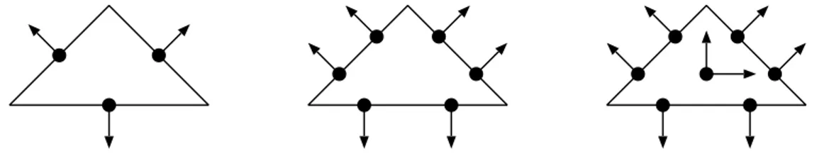
In Figure 1 we show the degrees of freedom for the Raviart-Thomas elements of order 0 and 1, and for the Brezzi-Douglas-Marini element of order 1.
Figure 1: Degrees of freedom for RT0 (left), BDM1 (center) andRT1 (right) on a triangle T.
We also introduce the standard Lagrange space of order m≥1:
Mh:=Lm(Th) = n
qh ∈ C(Ω)∩L20(Ω) : qh
T ∈ Pm(T), ∀T ∈ Th
o
.
The corresponding a priori error bound is given in the next theorem.
Theorem 3.1 Assume 0 < κ1 < kKk2 α
∞,ΩkK−1k2∞,Ω
and κ2 > 0. Then, if v ∈ [Ht(Ω)]d, div(v) ∈
Ht(Ω)and p∈Ht+1(Ω), there exists C >0, independent ofh, such that
||(v−vh, p−ph)||H ≤ C hmin{t,m,r+1}
||v||[Ht(Ω)]d+||div(v)||Ht(Ω)+||p||Ht+1(Ω)
.
Proof. It follows straightforwardly from the C´ea estimate (10) and the approximation properties of the corresponding finite element subspaces (cf. [16, 2]).
4
A posteriori error analysis
Let Hh×Mh be any finite element subspace of H(div,Ω)×M. Throughout this section, we
assume that 0< κ1 < kKk2 α
∞,ΩkK−1k2∞,Ω
,κ2>0 and we let (v, p)∈H0×M and (vh, ph)∈H0×Mh
be the unique solutions to problems (7) and (9), respectively. Then, we consider the residual
Rh(w, q) :=Fs(w, q)−As((vh, ph),(w, q)), ∀(w, q)∈H0×M. (11)
Using the ellipticity of the bilinear formAs(·,·) and the definition of the residual (11), we have
k(v−vh, p−ph)kH ≤ Cell−1
As((v−vh, p−ph),(v−vh, p−ph))
k(v−vh, p−ph)kH
≤ Cell−1 sup (w,q)∈H0×M
(w,q)6=(0,0)
As((v−vh, p−ph),(w, q))
k(w, q)kH
= Cell−1 sup (w,q)∈H0×M
(w,q)6=(0,0)
Rh(w, q)
k(w, q)kH .
(12)
In the next Lemma, we obtain an upper bound for the residual.
Lemma 4.1 There exists a positive constant C, independent ofh, such that
sup (w,q)∈H0×M
(w,q)6=(0,0)
Rh(w, q)
k(w, q)kH
≤ C||f− ∇ph− K−1vh||[L2(Ω)]d + ||ϕ−div(vh)||L2(Ω)
.
Proof. Let (w, q) ∈ H0 ×M. Using the definitions of the linear functional Fs and the bilinear
formAs(·,·), we can write
Rh(w, q) =R1(w) +R2(q), ∀w∈H0, ∀q∈M , (13)
where
R1(w) := Z
Ω
f·w +
Z
Ω
phdiv(w) − Z
Ω
K−1v
h·w − κ1
Z
Ω
(f− ∇ph− K−1vh)· K−1w
+κ2 Z
Ω
(ϕ−div(vh)) div(w)
(14)
and
R2(q) := Z
Ω
(ϕ−div(vh))q+κ1 Z
Ω
(f− ∇ph− K−1vh)· ∇q .
Then, integrating by parts the second term on the right hand side of (14), using thatw·n= 0 on Γ and applying the Cauchy-Schwarz inequality and the continuity ofK−1, we have
|R1(w)| ≤
(1 +κ1kK−1k)kf− ∇ph− K−1vhk[L2(Ω)]d + κ2kϕ−div(vh)kL2(Ω)
On the other hand, the Cauchy-Schwarz inequality also implies that
|R2(q)| ≤
κ1kf− ∇ph− K−1vhk[L2(Ω)]d + kϕ−div(vh)kL2(Ω)
kqkH1(Ω). (16)
Then, the proof follows by applying the triangle inequality in (13) and using (15) and (16). We remark thatC can be chosen as
C:= max(1 +κ1(1 +kK−1k),1 +κ2). (17)
Motivated by inequality (12) and the previous result, we define the a posteriori error estimator
ηh as follows:
η2h := X
T∈Th
ηh2(T), with ηh2(T) :=kf− ∇ph− K−1vhk2[L2(T)]d + kϕ−div(vh)k2L2(T).
We remark that the local error indicator ηh(T) consists of two residual terms, namely, the local
residual in Darcy’s law and the local residual in the mass conservation equation. We also notice that the global a posteriori error estimatorηhdoes not involve the computation of any jump across
the elements of the mesh. This fact, besides the good properties of the estimator stated in the next Theorem, makeηh well-suited for numerical computations.
Theorem 4.1 There exists a positive constant Crel, independent of h, such that
k(v−vh, p−ph)kH ≤ Crelηh, (18)
and there exists a positive constantCeff, independent of h and T, such that
Ceffηh(T) ≤ k(v−vh, p−ph)kH(div,T)×H1(T), ∀T ∈ Th. (19)
Proof. The first inequality is a consequence of (12), Lemma 4.1 and the definition of ηh. In
fact, we can takeCrel:=
√
2C/Cell, whereCell and C are the constants defined in (8) and (17),
respectively. On the other hand, we recall that div(v) = ϕ and f = ∇p+K−1v in Ω. Then, we
have that
||ϕ−div(vh)||L2(T)=||div(v−vh)||L2(T)
and, using the triangle inequality and the continuity ofK−1,
||f− ∇ph− K−1vh||[L2(T)]d ≤ max{||K−1||,1}
||v−vh||[L2(T)]d + ||∇(p−ph)||[L2(T)]d
.
Then, (19) follows withCeff−1 :=√3 max(1,kK−1k).
Theorem 4.1 establishes the equivalence between the total error and the estimatorηh. Inequality
(18) means that the a posteriori error estimatorηh is reliable, whereas inequality (19) means that
ηh is locally efficient. We remark that the efficiency constantCeff can be chosen independently of
5
Numerical results
In this section we present some numerical experiments that illustrate the confiability and efficiency of the a posteriori error estimator ηh. For implementation purposes, instead of imposing the
null media condition required to the elements ofMh, we fix the value of the pressure on a point
of the numerical domain. The non-homogeneous Neumann boundary condition is imposed by interpolation. The experiments have been performed with the finite element toolboxALBERTA(cf. [17]) using refinement by recursive bisection [12]. The solution of the corresponding linear systems has been computed using theSuperLU library [9]. We present numerical experiments for the finite element pairs (Hh, Mh) given by (RT0,L1), (RT1,L2) and (BDM1,L1) in the two-dimensional
case and (RT0,L1) in three dimensions.
We use the standard adaptive finite element method (AFEM) based on the loop:
SOLVE→ESTIMATE→MARK→REFINE.
Hereafter, we replace the subscripthbyk, wherekis the counter of the adaptive loop. Then, given a mesh Tk, the procedure SOLVE is an efficient direct solver for computing the discrete solution (vk, pk), ESTIMATE calculates the error indicators ηk(T), for all T ∈ Tk, using the computed
solution and the data. Based on the values of {ηk(T)}T∈Tk, the procedureMARK generates a set
of marked elements subject to refinement. For the elements selection, we rely on the maximum strategy: given a thresholdσ∈(0,1], elements T0∈ Tk such that
ηk(T0)> σ max T∈Tk
ηk(T), (20)
are marked for refinement. In our experiments, we fix σ = 0.6. Finally, the procedure REFINE creates a conforming refinementTk+1 of Tk, bisecting d times all marked elements (where d= 2,3 is the space dimension).
In what follows, we present three numerical experiments. The first one is devoted to study the robustness of the method with respect to the stabilization parameters,κ1 and κ2, and the rate of
convergence when the solution is smooth. In the two subsequent examples, we compare the perfor-mance of a finite element method based on uniform refinement (FEM) with the adaptive algorithm described above (AFEM). In Section 5.2, we study the performance of the AFEM algorithm when there are abrupt changes in the hydraulic conductivity tensor and the solution is not smooth. In Section 5.3 we consider an example in three dimensions. In all the examples, gravity effects are neglected, as it is often done in applications.
5.1 Example 1: Robustness and convergence rates
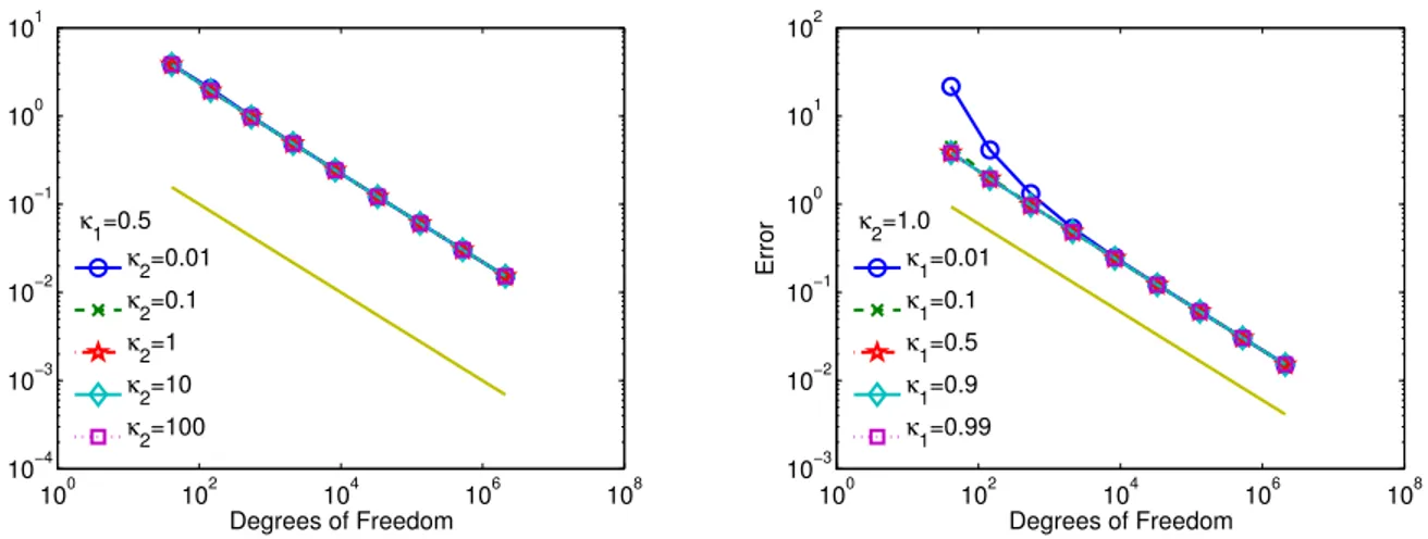
In order to study the robustness of the augmented scheme (9) with respect to the stabilization parameters and the sensitivity of the stabilized formulation to the ratio of the permeability to the viscosity, we consider an example with a smooth solution. We let Ω = (0,1)2 be the unit square, K= κµI,p(x, y) = sin(2πx) sin(2πy), f =0,v=−K ∇p,ϕ= div(v) and ψ=v·n.
We first consider K = I and investigate the effect of the stabilization parameters κ1 and κ2
100 102 104 106 108 10−4
10−3 10−2 10−1 100 101
Degrees of Freedom
Error
κ1=0.5
κ2=0.01
κ2=0.1
κ2=1
κ2=10
κ2=100
100 102 104 106 108
10−3
10−2
10−1
100
101
102
Degrees of Freedom
Error
κ2=1.0
κ1=0.01
κ1=0.1
κ1=0.5
κ1=0.9
κ1=0.99
Figure 2: Example 1. Decay of total error for κ/µ= 1 and several values ofκ1 and κ2.
decay of the total error versus the degrees of freedom (DOFs) for several values of κ1 and κ2, all
of them satisfying the hypotheses of Lemma 2.1. Optimal rates are attained in all cases, showing the robustness of the method with respect to the stabilization parameters.
According to these results, in what follows, we chooseκ1 = 2µκ and κ2 = 1.0. We remark that
these values of the stabilization parameters are consistent with the theory and ensure that the bilinear form As(·,·) is elliptic in the whole space. Then, we solve problem (9) using the finite
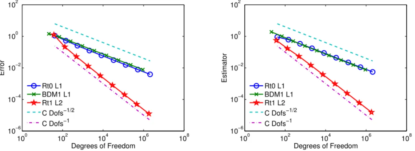
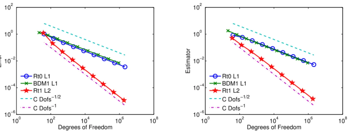
element pairs (RT0,L1), (RT1,L2) and (BDM1,L1) on a sequence of uniform meshes (i.e., in
each step all elements of the actual mesh are bisected twice). Figures 3, 4, 5 and 6 show the decay of the total error and the a posteriori error estimator versus the number of DOFs for κµ = 10−i,
i= 0, . . . ,3, respectively. We observe that the theoretical convergence rates predicted by the theory are achieved in all cases (we recall thath∼DOFs−1/don uniform meshes). Moreover, the estimator shows the same decay as the error.
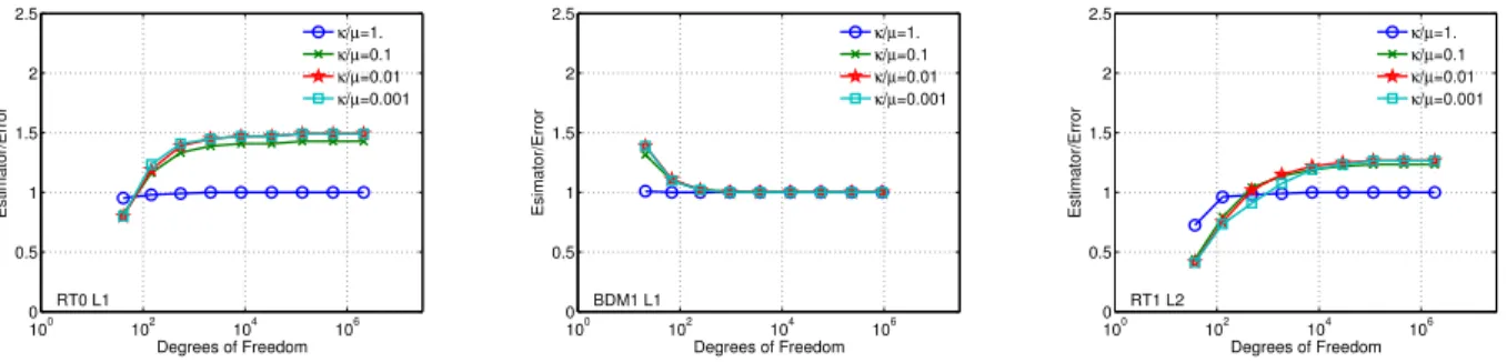
Finally, Figure 7 shows the efficiency indices (defined as the ratio of the estimated error to the total error) for the three finite element pairs considered here. As predicted by the theory, the efficiency index is bounded from below and above by positive constants, independently of the mesh size. In particular, when κ=µ, they approach one for the three discretization methods. We also remark that the efficiency indices obtained with theBDM1-discretization approach one in all cases.
This can be explained by the fact that the decay for theL2-norm of the velocity with the BDM1
method (h2 ∼ DOFs−2/d) is higher than for the H(div)-norm of the velocity (h1 ∼ DOFs−1/d). Since the contribution of theL2-norm of the error in the velocity in the total error is negligible for
smallh inBDM1, the estimator seems to be asymptotically exact in this case.
5.2 Example 2: A checkerboard configuration
100 102 104 106 108 10−6
10−4 10−2 100 102
Degrees of Freedom
Error
Rt0 L1 BDM1 L1 Rt1 L2 C Dofs−1/2 C Dofs−1
100 102 104 106 108
10−6
10−4
10−2
100
102
Degrees of Freedom
Estimator
Rt0 L1 BDM1 L1 Rt1 L2
C Dofs−1/2
C Dofs−1
Figure 3: Example 1. Decays of total error (left) and estimator (right) vs. DOFs for κ/µ= 1.
100 102 104 106 108
10−6 10−4 10−2 100 102
Degrees of Freedom
Error
Rt0 L1 BDM1 L1 Rt1 L2 C Dofs−1/2 C Dofs−1
100 102 104 106 108
10−6
10−4
10−2
100
102
Degrees of Freedom
Estimator
Rt0 L1 BDM1 L1 Rt1 L2
C Dofs−1/2
C Dofs−1
Figure 4: Example 1. Decays of total error (left) and estimator (right) vs. DOFs for κ/µ= 0.1.
at the origin. More precisely, we letKγ =a1(γ)Iin the first and third quadrants, andKγ =a2(γ)I
in the second and fourth quadrants. We consider Kellogg’s exact solution to the elliptic equation (cf. [11])
−div (Kγ∇p) = 0 in Ω, (21)
with appropriate Dirichlet boundary conditions for two different values ofγ, namely, γ = 0.50 and
γ= 0.25. For these values of the parameterγ, we have that
a1(0.50) =a1(0.25) = 1, a2(γ)∼=
0.171572875253810, ifγ = 0.50,
0.039566129896580, ifγ = 0.25.
Kellogg showed that an exact solution of (21) is given in polar coordinates by p(r, θ) = rγm(θ),
100 102 104 106 108 10−6
10−4 10−2 100 102
Degrees of Freedom
Error
Rt0 L1 BDM1 L1 Rt1 L2 C Dofs−1/2 C Dofs−1
100 102 104 106 108
10−6
10−4
10−2
100
102
Degrees of Freedom
Estimator
Rt0 L1 BDM1 L1 Rt1 L2
C Dofs−1/2
C Dofs−1
Figure 5: Example 1. Decays of total error (left) and estimator (right) vs. DOFs for κ/µ= 0.01.
100 102 104 106 108
10−6 10−4 10−2 100 102
Degrees of Freedom
Error
Rt0 L1 BDM1 L1 Rt1 L2 C Dofs−1/2 C Dofs−1
100 102 104 106 108
10−6
10−4
10−2
100
102
Degrees of Freedom
Estimator
Rt0 L1 BDM1 L1 Rt1 L2
C Dofs−1/2
C Dofs−1
Figure 6: Example 1. Decays of total error (left) and estimator (right) vs. DOFs forκ/µ= 0.001.
H1+γ−. Then, (vγ, pγ), withvγ =−Kγ∇pγ, is the exact solution of problem (3) when K =Kγ,
f =0,ϕ= 0 andψ=vγ·n.
We remark that the checkerboard pattern is the most demanding configuration in terms of regularity. We solve both problems with the finite element pair (RT0,L1) using uniform refinement
(FEM algorithm) and the adaptive refinement algorithm (AFEM) described at the beginning of this section. We chooseκ1(γ) = a2(γ)
3
2 and κ2 = 1.0, and fix to zero the value of the pressure in a
corner of the domain.
100 102 104 106 0 0.5 1 1.5 2 2.5
Degrees of Freedom
Estimator/Error
RT0 L1
κ/µ=1.
κ/µ=0.1
κ/µ=0.01
κ/µ=0.001
100 102 104 106
0 0.5 1 1.5 2 2.5
Degrees of Freedom
Esimator/Error
BDM1 L1
κ/µ=1.
κ/µ=0.1
κ/µ=0.01
κ/µ=0.001
100 102 104 106
0 0.5 1 1.5 2 2.5
Degrees of Freedom
Estimator/Error
RT1 L2
κ/µ=1.
κ/µ=0.1
κ/µ=0.01
κ/µ=0.001
Figure 7: Example 1. Efficiency indices for (RT0,L1) (left), (BDM1,L1) (center) and (RT1,L2) (right).
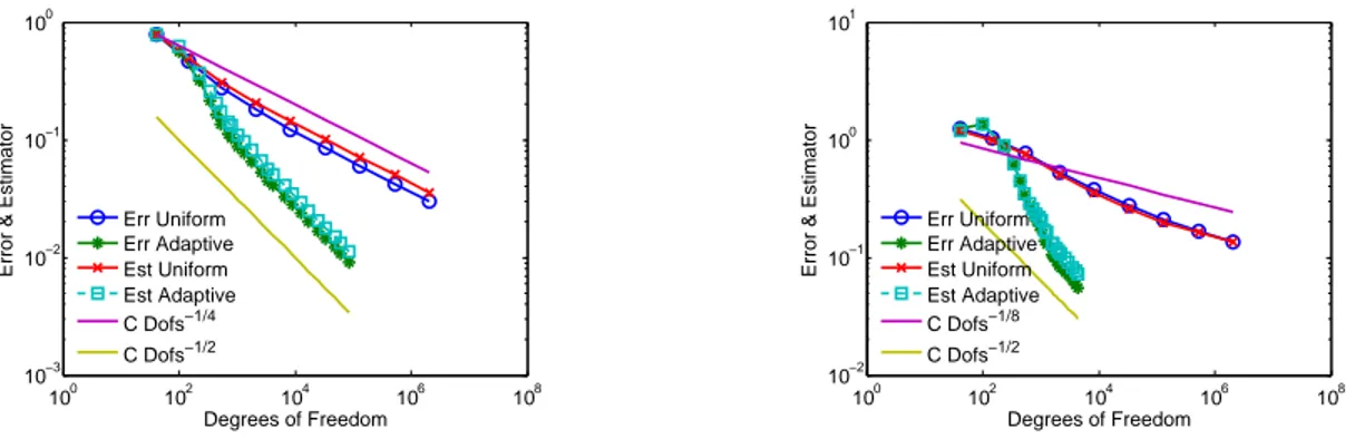
appears to be quasi-optimal. Efficiency indices are reported in Figure 9. There, we observe that they are bounded from above and below, which confirms that error and estimator are equivalent.
The adapted meshes obtained with this algorithm are highly graded at the origin, as can be observed in Figures 10 and 11 forγ = 0.50, and specially in Figures 12 and 13 forγ = 0.25.
Finally, in Figure 14 we present the pressure obtained after 20 AFEM iterations for γ = 0.5 (24128 triangles) andγ = 0.25 (1744 triangles). In Figure 15 we show the velocity fields obtained after 16 AFEM-iterations forγ = 0.50 (6228 triangles) and forγ = 0.25 (968 triangles). We observe that there are no oscillation in the pressure for the two values ofγ considered here, which confirms the stability of the method. We can also observe that the velocity is higher in the regions with greater values of the permeability.
5.3 Example 3: A three-dimensional simulation
This last example illustrates the performance of our algorithm on a five-spot type problem with a smooth solution. Let Ω = (0,1)3 be the unit cube. Motivated by Example 5.1 in [14], we choose the data of problem (3) so that the exact solution is (v, p), with
p(x, y, z) = log(tan2(Lr(x, y, z))),
where is a positive number, r(x, y, z) = p
(x+)2+ (y+)2+ (z+)2, L
= 2√3(1+2)π , and
v = −∇p (that is, K = I). We remark that there is a point sink at x = y = z = − and a point source atx =y =z = 1 +. However, since >0, the singularities are located outside the computational domain.
We recall that the five-spot problem can be modeled using a Dirac delta (as in [15]); however, we are interested in comparing the exact error with the a posteriori error estimator ηk. In order
to simulate the situation where source and sink are close to the boundary, we choose = 10−2.
The stabilization parameters are fixed to κ1 = 12 and κ2 = 1.0. We solve the problem for the
100 102 104 106 108 10−3
10−2 10−1 100
Degrees of Freedom
Error & Estimator
Err Uniform Err Adaptive Est Uniform Est Adaptive C Dofs−1/4 C Dofs−1/2
100 102 104 106 108 10−2
10−1 100 101
Degrees of Freedom
Error & Estimator
Err Uniform Err Adaptive Est Uniform Est Adaptive C Dofs−1/8 C Dofs−1/2
Figure 8: Example 2. Decays of total error and estimator vs. DOFs for (RT0,L1) with FEM and AFEM, forγ = 0.50 (left) andγ = 0.25 (right).
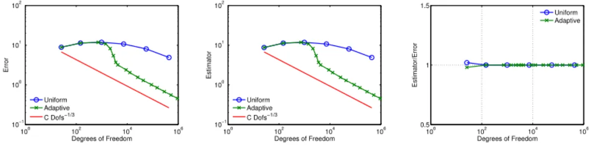
refinement algorithm is able to attain linear convergence, revealing itself as a very competitive algorithm. In this case (Figure 16, right), the estimator seems to be asymptotically exact.
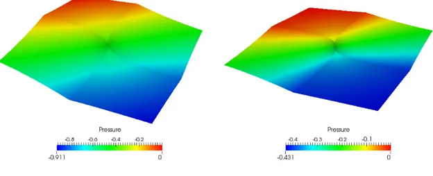
In Figure 17 we show some meshes generated by AFEM. We can see there that the meshes are highly refined near the singularity points, (−,−,−) and (1 +,1 +,1 +). Finally, in Figure 18 we show the pressure and the velocity fields obtained after 14 AFEM iterations (127578 tetrahedra).
6
Conclusions
100 102 104 106
0.5 1 1.5
Degrees of Freedom
Estimator/Error
Uniform Adaptive
100 102 104 106
0.5 1 1.5
Degrees of Freedom
Estimator/Error
Uniform Adaptive
Figure 9: Example 2. Efficiency indices for (RT0,L1) with FEM and AFEM, forγ = 0.50 (left) andγ = 0.25 (right).
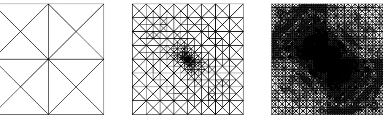
Figure 10: Example 2, γ = 0.50. Adapted meshes obtained after 0, 10 and 20 AFEM iterations, composed of 16, 880 and 24128 triangles, respectively.
Our main contribution is the derivation of a two-term a posteriori error estimator of residual type for the total error in this discrete scheme. The two residual terms account for the error in Darcy’s law and in the mass conservation equation. We remark that, besides the fact that it can be used with any finite element subspaces inRd (d= 2,3), this a posteriori error estimator is very
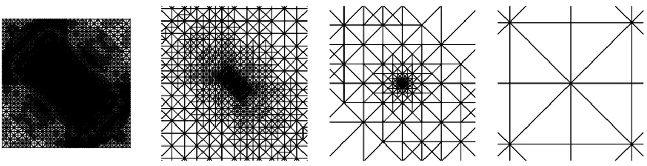
Figure 11: Example 2, γ = 0.50. Adapted mesh obtained after 20 AFEM iterations (24128 trian-gles). From left to right: full mesh and zooms to [−10−2,10−2]2, [−10−4,10−4]2and [−10−6,10−6]2.
Figure 12: Example 2, γ = 0.25. Adapted meshes obtained after 0, 10 and 20 AFEM iterations, composed of 16, 480 and 1744 triangles, respectively.
Figure 13: Example 2,γ = 0.25. Adapted mesh obtained after 20 AFEM iterations (1744 triangles). From left to right: full mesh and zooms to [−10−2,10−2]2, [−10−4,10−4]2 and [−10−6,10−6]2.
these theoretical results apply also to anisotropic porous media.
Figure 14: Example 2. Pressure obtained after 20 AFEM iterations forγ= 0.50 (left) andγ = 0.25 (right).
that the method is robust with respect to the stabilization parameters. Numerical experiments also illustrate the good performance of the adaptive algorithm based on the new a posteriori error estimator. Indeed, efficiency indices are close to one and the AFEM is able to localize the singularities and high-variation regions of the exact solution.
In the numerical analysis, we assumed that the Neumann boundary condition fits exactly. The effect of the approximation of the boundary datum will be analyzed in a forthcoming work. This approximation doesn’t seem to have an effect in the numerical experiments, at least for sufficiently regular boundary data (ψ∈L2(Γ)).
Acknowledgements. The authors would like to thank the anonymous reviewers for their com-ments and suggestions, that help to improve the paper. This research was partially supported by the Spanish Ministerio de Econom´ıa y Competitividad grants MTM2010-21135-C02-01, MTM2013-47800-C2-1-P, CGL2011-29396-C03-02 and CEN-20101010, by Consejer´ıa de Educaci´on (Junta de Castilla y Le´on, Spain) grant SA266A12-2 and by Direcci´on de Investigaci´on of the Universidad Cat´olica de la Sant´ısima Concepci´on.
References
[1] R.A. Adams and J.J.F. Fournier,Sobolev spaces. Academic Press, Elsevier, 2003.
Figure 15: Example 2. Velocity field (log-scale) obtained after 16 AFEM iterations for γ = 0.50 (left) andγ = 0.25 (right).
100
102
104
106
10−1 100
101 102
Degrees of Freedom
Error
Uniform Adaptive C Dofs−1/3
100
102
104
106
10−1 100
101 102
Degrees of Freedom
Estimator
Uniform Adaptive C Dofs−1/3
100
102
104
106
0.5 1 1.5
Degrees of Freedom
Estimator/Error
Uniform Adaptive
Figure 16: Example 3. Decays of total error (left) and estimator (center) and efficiency index (right) for (RT0,L1) with FEM and AFEM.
[3] F. Brezzi, M. Fortin and L.D. Marini, Mixed finite element methods with continuous stresses, Math. Models Methods Appl. Sci., vol. 3, pp. 275-287 (1993).
[4] F. Brezzi, T.J.R. Hughes, L.D. Marini and A. Masud, Mixed discontinuous Galerkin methods for Darcy flow, J. Sc. Comp., vol. 22-23, pp. 119-145 (2005).
Figure 17: Example 3. Adapted meshes obtained after 0, 8 and 16 AFEM iterations, composed of 6, 3840 and 420390 tetrahedra, respectively.
Figure 18: Example 3. Pressure and velocity field obtained after 14 AFEM iterations on a section of the domain (0,1)3.
[6] A.J. Chorin, Numerical solution of the Navier-Stokes equations, Math. Comput., vol. 22, pp. 745-762 (1968).
[7] M.R. Correa and A.F.D. Loula,Unconditionally stable mixed finite element methods for Darcy flow, Comput. Methods Appl. Mech. Engrg., vol. 197, pp. 1525-1540 (2008).
[8] H. Darcy,Les fontaines publiques de la ville de Dijon, Dalmont, Paris, 1856.
[9] J.W. Demmel, S.C. Eisenstat, J.R.Gilbert, X.S. Li and J.W.H. Liu,A super nodal approach to sparse partial pivoting, SIAM J. Matrix Analysis and Applications, vol. 20, pp 720-755 (1999).
[10] V. Girault and P.-A. Raviart, Finite Element Methods for Navier-Stokes Equations. Theory and algorithms, Springer-Verlag, 1986.
[11] R. B. Kellogg,On the Poisson equations with intersecting interfaces, Applicable Anal. 4, 101– 129, (1974/75).
[12] I. Kossaczky. A recursive approach to local mesh refinement in two and three dimensions, J. Comput. Appl. Math., vol. 55, no. 3, pp. 275288 (1994).
[13] M.G. Larson and A. M◦alqvist, A posteriori error estimates for mixed finite element approxi-mations of elliptic problems, Numer. Math., vol. 108, pp. 487-500, (2008).
[14] S.M.C. Malta, A.F.D. Loula and E.L.M. Garc´ıa,Numerical analysis of stabilized finite element method for tracer injection simulations, Comput. Methods Appl. Mech. Engrg., vol. 187, pp. 119-136 (2000).
[15] A. Masud and T.J.R. Hughes,A stabilized mixed finite element method for Darcy flow, Comput. Methods Appl. Mech. Engrg., vol. 191, pp. 4341-4370 (2002).
[16] J.E. Roberts and J.-M. Thomas,Mixed and Hybrid Methods, in Handbook of Numerical Anal-ysis, edited by P.G. Ciarlet and J.L. Lions, vol. II, Finite Element Methods (Part 1). North-Holland, Amsterdam (1991).
[17] A. Schmidt and K. G. Siebert. Design of Adaptive Finite Element Software: The Finite Ele-ment Toolboox ALBERTA, LNCSE 42. Springer (2005).