THE DYNAMIC COUPLING FACTOR FOR LONGITUDINAL MODES

THE ELECTROMECHANICAL COUPLING FACTOR FOR LONGITUDINAL

AND TRANSVERSE PROPAGATION MODES.

PACS: 43.38.Ar

Lamberti, Nicola1; Iula, Antonio2; Carotenuto, Riccardo2; Caliano, Giosuè2; Pappalardo, Massimo2.

1

Dipartimento Di Ingegneria Dell’Informazione e Ingegneria Elettrica, Università di Salerno Via Ponte don Melillo

84084 Fisciano (SA) Italy

Tel: +39 089 964305 Fax: +39 089 964218 E-mail: nlamberti@unisa.it 2

Dipartimento Di Ingegneria Elettronica, Università di Roma III Via della Vasca Navale 84

00146 Roma Italy

ABSTRACT

In the IEEE Standard on piezoelectricity the electromechanical coupling factor is defined in static conditions as the ratio between the converted and the total energy involved in a transfor-mation cycle (kmat). In this work we show that this definition can also be extended to dynamic

cases: by means of 1–D models we demonstrate that, for loss less piezoelectric elements vi-brating in the rod (longitudinal) or width (transverse) mode, the k factor can be defined as the square root of the ratio between the converted electric energy and the kinetic total energy; the obtained results are proportional to the appropriate kmat.

INTRODUCTION

The most important property of a piezoelectric material for practical applications is its ability to generate and to detect stress waves, i.e. to convert electrical energy into mechanical energy and vice versa. As it is well known, the electromechanical coupling factor k fully characterizes this energy conversion, taking the elastic, dielectric and piezoelectric properties into account; but, because these properties are strongly dependent on the electrical and mechanical bound-ary conditions of the piezoelectric element, many different k factors are defined in literature. More precisely, the kij, or the so-called material coupling factor (kmat) [1], refers to a

fundamen-tally one-dimensional geometry of the piezoelement and it is related to the converted energy in a static or quasi-static transformation cycle. The effective coupling factor keff refers to an

oscillat-ing specimen of any geometry, but it is not clear in the literature how it is related to the energies involved in a dynamic transformation cycle. Berlincourt et al. gave another definition of the cou-pling factor in their fundamental work on piezoceramics [2]. This definition can be applied in static and dynamic situations and it can be computed, in principle, for any geometry of the pie-zoelement, but it does not have a precise physical meaning and its relation with keff which,

can be defined as the square root of the ratio of the converted electrical energy to the total en-ergy involved in a transformation cycle, i.e. the kinetic enen-ergy; the value of the k factor com-puted in this way coincide with the one obtained using the empirical relation of the effective coupling factor keff which can be easily measured experimentally. In this work, by means of 1–D

distributed models, we demonstrate that these results can be applied to loss less piezoelectric elements vibrating in a longitudinal (for example rod) or a transverse (for example width) mode, and that the obtained results are proportional to the appropriate kmat.

THE DYNAMIC COUPLING FACTOR FOR LONGITUDINAL MODES

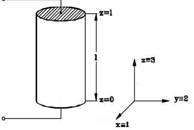
Let us consider, a piezoelectric bar of length l along z (or 3 direction), with its end faces elec-troded and with its cross section A of small diameter, compared with the length (see Fig. 1).

Fig. 1. Geometry of the piezoceramic rod vibrating in a (rod) longitudinal mode.

Suppose that the bar is made of piezoelectric ceramic, which belongs to the 6 mm symmetry class, polarised along the 3 direction. Because of the particular geometry and the electrical and mechanical boundary conditions, the element can be described by a one dimensional stress– strain system and therefore by two scalar constitutive equations [2]:

3 33 33 3 33 3

1

D s g S s T

D D −

=

3 33 3 33 33

3 S D

s g

E S

D + β

−

= ,

(1)

where:

2 33 33 33

33 33

33 33 33

d s

s ;

d

g _{E T}

E S

T = ₋

=

ε β

ε . (2)

The wave equation can be written as [2]:

2 2

3 2

33 2 2

3 2

1

z s

t D ∂

∂ = ∂

∂ ξ ξ

ρ , (3)

where ξ3 is the particle displacement in the z direction and the propagation velocity is:

. 1

33 3

ρ

D

s

v = (4)

By imposing stress–free conditions on the two terminal faces and supposing a sinusoidal excita-tion (D3 = D0 • e

jω t

3 3 3 3 3 33 3

2 v D

z cos tan v z sin v g                     −       = ω ϑ ω ω

ξ , (5)

where ϑ₃ =ωl/v₃. The particle velocity in the propagation direction z is the time derivative of the displacement: 3 3 3 3 3 33 3

2 v D

z cos tan v z sin v g j u                     −      

= ω ϑ ω , (6)

while the strain along z is the space derivative of ξ3:

3 3 3 3 33 3

2 v D

z sin tan v z cos g S                     +      

= ω ϑ ω . (7)

The electric field distribution can be computed by the second constitutive equation (1):

. D v z sin tan v z cos s g E D S 3 3 3 3 33 2 33 33 3 2 _                            +       −

= β ω ϑ ω (8)

By integrating the electric field along z between 0 and l (see Fig. 1), we obtain the voltage across the two electroded surfaces of the bar:

              − = 2 2 ₃ 33 2 33 3 33 3 ϑ ϑ β tan s g l D

V S _D (9)

The kinetic and the potential (converted) electrical energy densities can be computed by using (6) and (9):

(

)

4 1 2 1 3 2 3 3 3 2 3 2 33 2 0 0 2 / cos sin v g D dz u l w l k ϑ ϑ ϑ ϑ ρ ρ ₌ −

=

∫

2 2 2 1 2 1 2 3 33 2 33 3 33 33 2 0 2 0               − = = ϑ ϑ β

β s tan

g D V C l A w D S S

e , (11)

where C A/

( )

0 = β is the clamped capacitance of the element.

In the already cited paper [4] we demonstrated that, for a loss less piezoelectric element in free oscillation, mechanically and electrically insulated, the k factor can be defined as the square root of the ratio of we and wk. According to IEEE Standard on piezoelectricity [3], this ratio must

be computed when the element is fully insulated from the surrounding. The element is mechani-cally insulated, because we imposed stress free conditions, in order to solve the wave equation (3) and to compute the displacement (5); from an electrical point of view, the boundary condi-tions impose an exciting current and therefore the element can be considered electrically insu-lated when it vibrates at a frequency so that the input current goes to zero, or, equivalently, so that the electrical input impedance goes to infinity. The electrical input impedance is given by:

              − = 2 2 1 1 ₃ 33 33 2 33 3 0 ϑ β ϑ

ω s tan

g C

j

Zi _{D S} . (12)

As it can be seen from the previous equation, Zi goes to infinity for ϑ3 →π, i.e. for ù approach-ing the antiresonance frequency ù0 = ð v3 /l and it is evident from (10) and (11) that at this

2 2 2 33 2 33 33

2 33 2

2 8 8 8

lim

0

mat S

D k

e

w k k

s g w

w k

π π

β π ω

ω = = =

=

→ . (13)

As expected, the value of the dynamic coupling factor (kw) is less than the value of the static

factor (kmat), because in dynamic conditions not all the elastic energy is electrically coupled and

vice versa. The proportionality coefficient between kw and kmat is the same computed by

Berlin-court in [1] and relating keff and kmat; on the other hand, in the already cited paper [4], we

dem-onstrated that the effective coupling factor has the same value of the dynamic factor.

THE DYNAMIC COUPLING FACTOR FOR TRANSVERSE MODES

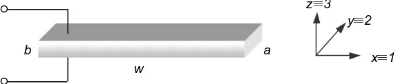
In order to show that the previous result is independent on the wave propagation direction, we now compute the dynamic coupling factor for a piezoelectric element vibrating in a transverse, for example in the width, mode. Consider a piezoelectric bar with its length w along the x–

direction, with the electroded faces normal to the z–direction (the polarisation direction) and with both cross–sectional dimensions a and b small compared with the length (see Fig. 2).

Fig. 2. Geometry of the piezoceramic element vibrating in a transverse (width) mode.

Because of the geometry, the electrical and mechanical boundary conditions, the element can be described by the two scalar constitutive equations [2]:

3 31 1 11

1 s T d E S = E +

3 33 1 31

3 d T E

D = + εT . (14)

The wave equation can be written as [2]:

2 2

1 2 2 1 2 2

1 2

x v

t ∂

∂ = ∂

∂ ξ ξ

, (15)

where ξ1 is the particle displacement in the x direction and the propagation velocity is:

. s

v _E1

11 1

ρ

= (16)

By imposing stress–free conditions on the two faces orthogonal to the x axis (the element is therefore mechanically insulated) and supposing a sinusoidal excitation (E3 = E0 • e

jω t

), the so-lution of the wave equation (15) is:

3 1 1

1 1

31 1

2 v E

x cos tan

v x sin v d

    

  

            −      

= ω ϑ ω

ω

ξ , (17)

where ϑ1=ωw/v1. The particle velocity in the x propagation direction is the time derivative of the displacement:

w

a b

3 1 1 1 1 31 1

2 v E

x cos tan v x sin v d j u                     −      

= ω ϑ ω , (18)

while the strain along x is the space derivative of ξ1:

3 1 1 1 31 1

2 v E

x sin tan v x cos d S                     +      

= ω ϑ ω . (19)

The electric displacement can be computed by the second constitutive equation (14):

(

)

1 1 1 2 31 33 2 31 33 3 2 1 E v x sin tan v x cos k k

D T T

                            +       + −

= ε ε ω ϑ ω , (20)

where E T _s k 11 33 31 31 d ε = ₍₂₁₎

is the static (material) coupling factor for this vibration mode [2].

By differentiating the electric displacement with respect to the time and integrating along the x–y

plane (see Fig. 2), we obtain the current in the specimen:

3 1 1 2 31 2 31 33 2 2

1 k k tan E

w a j

I T _

           + − = ϑ ϑ ε

ω . (22)

The kinetic energy density can be computed by using the (18):

(

)

=

∫

For this vibration mode the potential (converted) electrical energy must be computed taking the current I into account, because the voltage V represents the electrical excitation:

2 2 1 2 1 2 1 2 0 2 1 1 2 31 2 31 33 2 0w 2 E tan k k C I w b a

w_e T _

           + − = = ϑ ϑ ε

ω , (24)

where C0w =εT33

( )

To compute the k factor we must ensure that the element is also electrically insulated; in this case the electrical boundary conditions impose an exciting voltage and therefore the element can be considered insulated when the input voltage goes to zero, or, equivalently, when the electrical input admittance goes to infinity. The electrical input admittance is given by:

            + − = 2 2 1 1 1 2 31 2 31 0 ϑ ϑ

ωC k k tan

j

Y_{i w} . ₍₂₅₎

In the previous equation it is evident that Yi goes to infinity for ϑ1→π, i.e. for ù approaching the resonance frequency ù0 = ð v1 /w; as expected, at this frequency both the kinetic and

elec-tric energies go to infinity (see (23) and (24)), because we considered a piezoceramic element without losses. In order to obtain the kwfor this vibration mode we, also in this case, compute:

2 2 2 31 2

2 8 8

lim

0

mat k

e

w k k

w w k π π ω ω = = =

Comparing the expression of the dynamic coupling factor computed for this vibration mode with the expression obtained for the longitudinal mode (see (13)), we can observe that the relation between kw and kmat is the same in both cases. We can therefore conclude that, for a one

di-mensional vibration mode (longitudinal or transverse), the dynamic coupling factor is related to the so-called material factor by the proportionality coefficient 8/ð2.

CONCLUSIONS

In this paper we have computed the dynamic coupling factor of two piezoelectric elements vi-brating in the rod and the width mode respectively. By means of the appropriate 1–D distributed models, the k factor was computed according the definition given in [4], i.e. as the square root of the ratio between the converted electrical energy and the kinetic energy — the total energy in-volved in a transformation cycle. In both cases we obtained that the dynamic coupling factor is related to the appropriate material coupling factor by the proportionality coefficient 8/ ð2. We can therefore conclude that this definition of the dynamic coupling factor can be applied to any one dimensional vibration mode (longitudinal or transverse) of a loss less piezoelectric element. In the future we think to extend this definition to multi dimensional elements and to take the ma-terial losses into account.

BIBLIOGRAPHICAL REFERENCES

[1] D. A. Berlincourt, “Piezoelectric Crystals and Ceramics,” in Ultrasonic Transducer Materials, O. E. Mattiat, Ed. New York: Plenum Press, 1971, pp. 63–124.

[2] D. A. Berlincourt, D. R. Curran and H. Jaffe, “Piezoelectric and Piezomagnetic Materials and Their Function in Transducers,” in Physical Acoustic, vol. 1, W. P. Mason, Ed. New York: Academic Press, 1964, pp. 169–270.

[3] IEEE Standard on Piezoelectricity, ANSI/IEEE Std 176–1987. New York: The Institute of Electrical and Electronics Engineers, 1987.