Sources of income persistence: evidence from rural El Salvador

C

C

|

E

_E

|

D

_D

|

L

_L

|

A

_A

|

S

_S

Centro de Estudios

Distributivos, Laborales y Sociales

Maestría en Economía Universidad Nacional de La Plata

Sources of Income Persistence: Evidence from Rural

El Salvador

Walter Sosa-Escudero, Mariana Marchionni y Omar

Arias

Sources of Income Persistence:

Evidence from Rural El Salvador

Walter Sosa-Escudero, Mariana Marchionni, and Omar Arias

May 2006

Abstract. This paper uses a unique panel dataset (1995-2001) of rural El Salvador to investigate the main sources of the persistence and variability of incomes. First we propose an econometric framework where a general dynamic panel model is validly reduced to a simple linear structure with a dynamic covariance structure, which augments considerably the number of degrees of freedom usually lost in the construction of instruments to estimate standard dynamic panel models. Then we investigate the extent to which families are continuously poor due to endowments (observed and unobserved) that yield low income potential or due to systematic income shocks that they are unable to smooth. We find that life-cycle incomes are largely explained by the relatively time-invariant productive characteristics of families and their members such as education, public goods and other assets. Observed income determinants account for about half of income persistence. Controlling for unobserved heterogeneity leaves little room for pure state dependence. Although of second order, high volatility and the inability to insure from shocks is a more important source of variation in incomes than in developed countries. Low income potential is the more likely source of poverty traps in Rural El Salvador. Many of the family endowments are manipulable by policy interventions, although many not in the short term.

Key Words: Income mobility, Poverty Traps, Panel Data, El Salvador.

JEL code: I32

1

1 Introduction

Despite significant structural economic reforms growth has been scant and poverty and inequality remain high and deep-rooted in Latin America and the Caribbean (LAC

henceforth). Around 40 percent of the region’s population has lived in poverty

measured according to country-specific living standards since the mid-1990s.2 And because of population growth the number of poor actually increased in the early 2000s.

A key question for public policy is whether this lack of progress in poverty results from the persistence of poverty in the same families or from movements

in-and-out of poverty of different families. Income deprivation is perceived as a greater

concern when it is persistent over time rather than transitory. Moreover, policy

interventions should have a different emphasis depending on which is the main source

of low-income persistence; poverty due to high income volatility calls for interventions

to reduce and insure risks while poverty arising from insufficient endowments requires

policies to increase income potential.

This issue concerns the literature of intergenerational income mobility and more

recently of poverty vulnerability. In essence both address the question: how likely is it

that a household of given characteristics finds itself in poverty at a given future time?.

The answer ultimately depends on the long-term consumption prospects and

consumption volatility faced by a household. That is, a household can be persistently

poor due to endowments that yield low income potential and/or due to income shocks

that it is unable to smooth. Thus, income persistence depends on the state and evolution

of household characteristics (observed and unobserved) and of the aggregate

environment.

The subject naturally requires data following households over a relatively long

time span, which has hindered research in Latin America.3 To this purpose, this paper uses a unique panel dataset (1995-2001) for rural El Salvador to investigate the main

sources of the persistence and variability of incomes, offering a valuable opportunity to

study these issues in Latin America. The country achieved considerable improvements

in poverty and other living conditions indicators during the 1990s. Rural poverty fell by 20 points according to official data (World Bank 2005). Recent studies (See World

Bank 2005) have shown that much of this progress is related to a significant economic

2

This figure is based on national poverty lines (the cost of country specific baskets of basic food and non-food consumption) estimated in the Socio-economic Database for Latin America and the Caribbean (SEDLAC) maintained by the LAC World Bank poverty group and the Center for Distributional, Labor and Social Studies (CEDLAS) of the University of La Plata in Argentina (see World Bank 2006 and www.depeco.econo.unlp.edu.ar/cedlas).

3

diversification from traditional agriculture (i.e., basic grains, coffee and sugar) to

off-farm productive activities, important investments in rural infrastructure that improved access to markets, and an important inflow of international remittances.

Notwithstanding, El Salvador was affected by several shocks, particularly sequels of the

Mitch storm, the drought caused by the El Niño effect, two earthquakes, and a fall in

coffee export prices. Half of Salvadorians in rural areas remain poor and a quarter live

in mere subsistence. Thus, El Salvador offers important insights on the mechanics of

income and poverty dynamics in a context of significant poverty reduction driven by

private strategies and public investments.

From a methodological point of view, this paper uses a linear specification

similar to that used in the classic Lillard and Willis (1978) study, where the relevant

dynamic components are modeled as part of the covariance structure of a linear panel

data model. A methodological contribution of this paper is to show that this particular

specification is a valid restriction of a general dynamic panel linear model. The main

advantage of adopting this simplification is the considerable savings in terms of degrees

of freedom arising from the fact that the dynamic covariance structure can be handled

by a simple method-of-moments, unlike standard linear dynamic panels which require

instrumental variables implying a considerable loss in degrees-of-freedom, a much relevant issue when, as in our case, the time dimension of the problem is short. The

paper uses the framework proposed by Bera, Sosa-Escudero and Yoon (2001) to

formally test the relevance of the dynamic covariance model.

The paper is organized as follows. The next section presents a brief review of the

relevant literature. Section 3 describes the panel data set used. Section 4 discusses the

econometric strategy used in the paper. Sections 5 and 6 discuss the results of the econometric analysis and some simple exercises that help interpret them. Section 7

concludes and highlights the main implications for public policy.

2 The empirical evidence on income persistence

Taking household income as determined by the retribution to the use of all the

assets owned by a family, life-cycle incomes reflect the evolution of these assets, their

pricing, and how both are affected by economic and other shocks. Friedman and

Kuznets (1954) first proposed the decomposition of the determination of incomes over

time into permanent and transitory components, which became later embedded in

Friedman’s permanent income hypothesis. Since then the intergenerational income mobility literature has focused on the role of assets and their returns to explain

where longer panel data allows studying this phenomenon. As exemplified below, the

strand of studies on poverty vulnerability is more common in developing countries where short panels or cross-section data have been used to examine the link between

poverty and the inability to smooth out the kinds of shocks that are prevalent in regions

like LAC.

In their seminal work, Lillard and Willis (1978) conducted a careful empirical

study of life cycle earnings mobility using U.S. data from the Panel Survey of Income

Dynamics (PSID), clearly rooted in Friedman and Kuznets’ framework. They developed and estimated a dynamic reduced form model of earnings with a deterministic

component consisting of a trend, a vector of observed family characteristics and an

unobserved family specific effect, as well as a transitory shock modeled as a first order

autoregressive process. The permanent component reflects a family’s long-term income

potential related to its productive characteristics such as human capital, other assets, and

family specific unmeasured skills. The transitory component captures external factors

such as economic swings, idiosyncratic shocks, or plain measurement errors, which

make incomes depart from their permanent level. Their main findings are that low

earnings at early ages are strong predictors of low earnings later in life, even

conditioning on observed individual characteristics, and that income shocks (“bad luck”) have a secondary role in explaining long-term income mobility. They found that

in a given year, most of the variance in earnings not accounted for by family and

individual factors (such as race, education and age) is due to transitory shocks, but that

over a lifetime the bulk of income persistence is due to unobserved individual

heterogeneity.

These key results have endured different estimation and testing methods and studies, and updated data sets. The seminal work of MaCurdy (1982) shows that earnings

from the PSID are best described by the sum of a random walk and an MA(1) component. Abowd and Card (1989), Gottschalk and Moffitt (1994), Meghir and Pistaferri (2002),

as well as more recent applications using semiparametric and Bayesian methods

(Horowitz and Markatou (1996); Geweke and Keane (2000)) find similar results and

further develop these ideas.

A parallel literature on vulnerability has analyzed similar issues in terms of

families’ future consumption prospects for given endowments (observed and

unobserved) and the risks to actually materialize those prospects. Examples are

Chaudhuri, Jalan and Suryahadi (2002), Chaudhuri (2000), Pritchett, Suryahadi and

The absence of mobility or inability to recover from severe shocks also lie in the

realms of the poverty traps literature where individuals, communities, or even nations are unable to escape from poverty or a low level of development (Azariadis and

Stachurski, 2005). This may occur due to the presence of a minimum scale of

production before an investment becomes profitable, credit constraints or excessive

underinsured risk under imperfect financial markets, or the inability to exploit

complementarities in production between human, physical, or social assets. Lokshin

and Ravallion (2004) examine income dynamics in Hungary and Russia using a six year

and four year panels, respectively, and they propose a simple way of identifying poverty

traps. They estimate the degree to which the relationship between present and past

incomes involves a polynomial function that embeds a hump or income threshold below

which families become “trapped” in a low income equilibrium. They find significant

evidence of nonlinearities in income dynamics in these two countries, but no evidence of dynamic poverty traps, that is, of a threshold income level below which income

deprivation persists. Their results also highlight that measurement error in incomes,

which are likely aggravated in short data panels, is likely to cause spurious negative

correlation between income changes and initial levels. More recently, Newhouse (2005)

estimates the persistence of transient income shocks in rural Indonesia and found that

more permanent causes of household poverty such as endowments are more significant

and that measurement error in income and unobserved household heterogeneity are

important sources of bias.

As stressed in the introduction, the analysis of these issues in Latin America and

the Caribbean has been scant due to insufficient panel data. For instance, Fields et. al.

(2005) use panel data for Argentina, Mexico and Venezuela, to examine changes in

individual earnings during one to two year spells of positive and negative economic

growth. They find limited evidence (except somewhat for Mexico) for what they call

“divergent mobility”, by which those that start off relatively better off experience the

largest earnings gains or smallest income losses. Their results are thus inconsistent with

poverty traps. To our knowledge Freije and Souza (2002) is the only study that uses the Lillard and Willis (1978) methodology to analyze income mobility in the region. They

use a two-year panel for Venezuela and found that, in any given year, the majority of

variation in incomes is not accounted for by education or observed family

characteristics but instead is due to transitory shocks. That is, volatility is the major

source of variation in incomes across families, contrary to the findings for developed

countries.

However, a problem plaguing this and related studies in LAC is their reliance on

are likely to disproportionately capture measurement error or short term income

variation rather than the longer term income mobility of prime interest in the intergenerational mobility and poverty traps literature. This is confirmed in the studies

by Lokshin and Ravallion (2004) and Newborne (2005).

Two recent studies have tried to circumvent this problem. Rodríguez-Meza and

González-Vega (2004) study income dynamics and test for the presence of poverty traps

using the same 7 year panel data for El Salvador we use in this paper. They adopt an

approach similar to Lokshin and Ravallion (2004) and found evidence of non-linearities in income dynamics consistent with the existence of poverty traps. Although higher

income families in rural areas recover very quickly from an income shock the poor face

a much longer time to recover. In fact, the prospects of very low income families (ie.,

in extreme poverty) to escape subsistence levels become very dim after being hit by a

catastrophic income shock. This result, however, might not be robust since, as the

findings of Lokshin and Ravallion (2004) attest, tests of highly non-linear income

processes that use a few years of panel data are likely to have reduced power to

distinguish among alternative income dynamic specifications. Another approach

proposed by Antman and Mckenzie (2005) relies on pseudo panels to track cohorts over

repeated cross sectional surveys to measure income mobility among “representative” individuals moving across time. This approach effectively averages out transitory

shocks across an entire cohort thus correcting for measurement error in incomes. They

find little evidence for poverty traps in Mexico and significantly lower measured

mobility in the pseudo panels compared to the actual panel transitions. However, none

of these two studies explicitly analyze the relative contribution of the permanent and

transitory income components to income mobility or the persistence of low income

states.

In this paper we reexamine the question of income mobility exploiting the

advantages of the longer-span of panel data for El Salvador and the parsimonious linear

dynamic income model of Lillard and Willis (1978). We test and find supporting

evidence that this conveniently simplified model is an econometrically valid reduction

that uses more efficiently the relatively longer but still short span of data. Moreover, the

proposed framework allows a richer investigation of a number of policy-relevant

questions such as do families starting with a low income status in 1995 in El Salvador

have a high chance of still being low income in 2001? Which factors make low income

states to be transitory for some households and permanent for others? How much hinges on idiosyncratic and transitory characteristics of families (measured and unmeasured) or

unexploited externalities like absent public goods and how much on external shocks or

3

The data

We use data from the rural panel survey (BASIS hereafter) conducted by the Fundación

Salvadoreña para el Desarrollo Económico y Social (FUSADES) and the Rural Finance

Program at the Ohio State University (OSU). The survey collects data on incomes,

demographic, occupational, access to credit and physical assets (e.g., infrastructure,

land, housing) among other characteristics of rural households and their strategies to

cope with risk (for further details on the survey and data see Rodríguez-Meza and

González-Vega (2004)). The panel data set is composed of four biennial observations

for the years 1995, 1997, 1999, and 2001. While still a limited time span, this is a major

improvement over the one to two year panels that have been used to study mobility in

LAC.

In 1995, 628 households were interviewed while in 2001 only 450 of the original

households remained in the panel, reflecting an accumulated attrition rate of 28 percent.

More than 75 percent of the attrition occurred from the first to second wave when it was

decided the survey would be continued as a panel. We focus the analysis on households

since this is a more relevant unit of analysis for assessing intergenerational income

mobility and also minimizes concerns arising from panel attrition which is more prevalent among individuals. A total of 449 households are observed in all four years,

but we have complete information only for 409 which will be the main sample used in

our analyses.

The evolution of incomes has been more favorable for off-farm income sources.

Table 1 shows the level and growth rate of annual per capita income at different percentiles of the household income distribution (using only the cross-section structure

of the data). Between 1995 and 2001, the average family per capita income grew at an

average rate of 8% per year The evolution of incomes has been relatively more

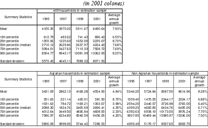
Table 1. Evolution of annual per capita income of Rural Households in El Salvador

(in 2001 colones)

1995 1997 1999 2001

Average annual growth Mean 4105.35 3975.02 5911.67 6490.64 7.93%

10th percentile 612.79 483.62 741.43 896.43 6.55% 25th percentile 1355.06 1225.60 1653.00 2235.07 8.70% 50th percentile (median) 2710.12 2629.86 3637.97 4224.43 7.68% 75th percentile 5084.01 5427.63 7113.33 7928.72 7.69% 90th percentile 8304.77 8943.17 13081.99 13362.00 8.25%

Standard deviation 5575.45 4645.11 7089.32 8071.50

1995 1997 1999 2001

Average annual growth

1995 1997 1999 2001

Average annual growth Mean 3431.09 2862.13 4168.28 4554.93 4.84% 5346.20 5724.84 8387.50 8614.96 8.28%

10th percentile 351.63 221.14 430.01 581.50 8.75% 1559.40 1470.55 2244.17 2324.17 6.88% 25th percentile 1031.63 784.72 1169.21 1303.67 3.98% 2594.20 2440.57 3726.98 3765.00 6.40% 50th percentile (median) 2088.30 1824.76 2405.69 2696.41 4.35% 4399.25 4660.83 6434.76 6495.00 6.71% 75th percentile 4012.64 3449.50 4836.84 4608.00 2.33% 6392.63 6938.10 10173.05 9976.24 7.70% 90th percentile 7386.97 6234.80 8540.59 9456.05 4.20% 9937.85 10499.44 15985.97 15336.00 7.50%

Standard deviation 5806.09 3898.06 5744.42 7286.53 4905.49 5170.17 8037.65 8369.70 Non-Agrarian households in estimation sample Summary Statistics

Agrarian households in estimation sample 409 households in estimation sample Summary Statistics

Source: Own estimates based on BASIS (1995-2001).

Numerous analyses with this dataset indicate that assets endowments (land,

education), access to markets and infrastructure (road, credit), household risk coping

strategies (productive diversification, microenterprise development, remittances), and

household demographics (size, composition, gender) all affect family income growth.4 In this paper we focus on the sources of income persistence, and thus on what explains

that some families are able to experience more income mobility than others.

4

Econometric modeling of income persistence

The relatively short time span of the panel casts some doubts on the adequacy of

standard dynamic panel model analysis of these data. This section discusses a

convenient simplification that, under valid restrictions, can be informative about the

questions of this paper while using the available information efficiently.

4

Let yi,t denote income of household i in period t. When incomes are stationary, a

simple measure of short term persistence is the (unconditional) correlation of incomes between adjacent periods, Cor(yi,t, yi,t-1). A basic goal of the analysis is to compare this

total correlation with the partial correlation that arises after controlling for exogenous

determinants (family specific or not) and non-observed family specific factors. A

standard specification that accommodates all these factors is the linear dynamic

equation:

yi = γ yi,t-1 + xi,t' β0 + xi,t-1'β1 + µi + εit (1)

where i=1,…,N households, and t=1,…,T, periods, xi,t is a K vector of observed

exogenous determinants of income, µi is a zero mean random variable representing

unobserved, family specific terms, and εit is a white noise process representing family

and time specific unobserved shocks.5

A relatively well established fact is that empirical models for individual and

family income have a rather low explanatory power even when a rich micro-data base is

used, which renders unobservable “error terms” as very important determinants of

income.6 These include family specific, non-measured variables like, for example, unmeasured skills, preferences, and risk aversion, which is associated with unobserved

heterogeneity in panel models and generally considered to be persistent over time.

Time-variant-family-specific shocks can also be persistent. For example, it takes time to recover from a job loss or death of a family working member or to rebuild human

capital that due to sudden changes in technology becomes quickly obsolete. These can

generate “state dependence”, that is, an income fall in a low income state in a given

period increases the chances of being low income in subsequent periods.

An important aspect of the analysis is to distinguish between these different sources of income persistence given their distinct policy implications. Persistence due to

insufficient endowments (observed and unobserved) requires policies to increase

income potential such as health, educational and infrastructure investments. Persistence

of shocks under high income volatility calls for interventions to reduce and insure risks

such as safety nets and improved access to financial markets.

5

This model has also found applications in the literature of persistence of regional unemployment literature. See Blanchard and Katz 1992 and more recently Galiani, Lamarche, Porto and Sosa-Escudero 2005.

6

Estimates of (1) can provide a measure of what part of total income persistence

remains when various sources of persistence are accounted for since γ is a partial

correlation.7 Consistent estimation of the parameters γ, β0 and β1 has been well studied

in the econometrics literature. The case when γ is different from zero renders standard

estimators inconsistent requiring alternative strategies like GMM methods (Arellano and Bond 1991). Moreover, there is ample evidence on the poor sample performance of

GMM based estimators (e.g., Judson and Owen 1999) in terms of bias and efficiency

when T is small. This highlights the relevance of adopting valid simplifications to

increase the reliability of estimates in our case where only four time-observations are

available.

In their seminal paper Lillard and Willis (1978) proposed a very appealing

approach that relies on autocorrelated models as convenient simplifications of more

general dynamic structures, much in the spirit of the classic paper by Hendry and Mizon

(1978). Consider a simple linear panel data model with first order autocorrelation:

yit = xit'δ + µi + vit (2)

vit = φ vi,t-1 + it, |φ| < 1 (3)

where µi ~ iid (0, σ2µ), it ~ iid (0, σ2), independent of each other and of xit. In this

specification the potential sources of persistence are xit, µi and the presence of serial

correlation in the observation specific error process. The vector µi represents in our case

family-specific unobserved heterogeneity, and the serially correlated structure in the

error term represents 'state dependence' of the shocks to family incomes. This is

basically the same setup used in Lillard and Willis (1978) and we refer to this paper for further references. The parameters of this model can be estimated by

maximum-likelihood methods under suitable distributional assumptions, as in Lillard and Willis

(1978), or by relying on the method of moments as in Baltagi (2001, pp.82-83).

It can be readily verified that the serially correlated model in (2)-(3) is a

particular, testable restriction of the linear dynamic model in (1). Substract φ yi,t-1 in

both sides of (2) and simplify using (3) to get:

7

yit = φ yi,t-1 + xit'δ - φ xi,t-1'δ + (1- φ) µi + it (4)

This is basically model (1) with the non-linear restrictions:

-β1k / β0k = γ, k=1,…,K (5)

which can be subject to standard Wald-type tests after estimating the unrestricted model. The practical advantages of considering these restrictions implicit in Lillard and

Willis (1978) is that their model can be estimated using N(T-1) observations, whereas

the differencing and instrument construction process of GMM related estimators is

based on N(T-3) observations, which would infringe a significant loss of degrees of

freedom in the El Salvador data set.

A convenient advantage of the simple structure implicit in (2)-(3) is that measures of the variation and persistence of incomes can be conveniently summarized

in a simple parametric fashion. Let the composite unobservable error terms be uit ≡ µi +

vit, and let σ2v denote the variance of vit, which, given the AR(1) structure of v, is given

by σ2v = σ2 / (1- φ2). Hence the total variation in incomes arising from unobservable

factors is σ2u = σ2µ + σ2v = σ2µ + σ2 / (1- φ2). Also λ≡σ2µ / σ2u measures the relative

importance of the family specific components in the overall variance of the error term.

Another magnitude of interest is the autocorrelation of the overall error term, which can

be easily verified to be given by:

ρs≡ Cor(uit,ui,t-s) = λ + (1- λ) φs (6)

Hence, income persistence arising from unobservables is an average of the

persistence induced by family-specific time invariant factors and period specific shocks,

weighted by their relative importance in explaining income variations. If σ2=0 the pairwise temporal correlation of the composite error terms is trivially one (due to the

presence of unobserved heterogeneity), whereas if σ2µ =0 the only correlation left is the

one induced by the serially correlated, observation specific income shock. This means

that if the interest lies in persistence, the relative importance of each source depends on

how large is the persistence of each source and how important is that particular source

overall income persistence. The inclusion of explanatory variables has the effect of

netting out the income persistence induced by observable income determinants.

Tests of the restrictions embodied in (2)-(3) can be conducted under the

comprehensive testing framework for serially correlated models with unobserved

heterogeneity of a recent study by Bera, Yoon and Sosa Escudero (2001). Their

proposed tests are conveniently based on estimation under the joint null σ2µ = 0 (no

random effects) and φ= 0 (no serial correlation) by pooled OLS. Additionally, they

correctly detect whether persistence is due to the presence of unobserved heterogeneity, serially correlated shocks or both, unlike standard tests which confound one effect with

the other. For example, the standard Breusch-Pagan test for random effects tends to

reject the null hypothesis under the presence of unobserved heterogeneity and/or the

serial correlation, which makes it unattractive to detect which is the main source of

persistence. The fact that Bera et al’s procedure is based on pooled OLS using N(T-1)

observations should increase testing power compared to direct estimation of the full

dynamic model to test H0: γ = 0 (no dynamic effect) using N(T-3) observations. Still,

this would require the implementation of an appropriate test for H0: σ2µ = 0 (no

unobserved heterogeneity).

Consequently, our empirical strategy consists of the following steps:

1. Start by implementing the Bera et al. (2001) testing procedure to elucidate the

validity of the stochastic restrictions in (2)-(3), that is, whether one or both

sources of persistence are present. We estimate a model under the joint null

hypothesis. Recent work by Zincenko (2005) shows that the modified test of

Bera et al. (2001) has power in the direction of HA : γ = 0 in the dynamic

model.

2. Under the presence of dynamic effects, the dynamic model will be estimated

with the purpose of obtaining a basic set of estimates of the relevant parameters

and to test the non-linear restrictions described above.

3. Under the null of valid restrictions, the Lillard-Willis (1978) simplification will

be adopted, and the full error component with serial correlation will be

estimated using the method-of-moments approach described in Baltagi (2001).

This strategy provides estimates of all the parameters of interest.

A remaining concern is the bias arising from sample attrition

(individuals/families dropping from the panel) due to the correlation between the

suffering catastrophic income shocks may be more likely to breakup or more risk-taking

families may be more likely to migrate, which could lead to dropping out of the panel survey. As highlighted by Lokshin and Ravallion (2004) this is an important potential

source of biases in this type of analysis. The attrition rate is 28 percent among families,

and largely occurred from the first to second wage when it was decided the survey

would be continued as a panel. The evidence from previous studies indicates that this

does not appear to affect significantly the sample composition and the validity of

statistical inference from this sample (see Rodríguez-Meza and Gonzalez-Vega 2004).

5 Empirical results

Following the previous studies using these data, the empirical models include a multitude of characteristics standard in the literature of microdeterminants of family

incomes. In particular, we follow closely the empirical specifications recently adopted

by Tannuri-Pianto, Pianto, Arias and Beneke de Sanfeliu (2005) who carry a

comprehensive study of the microdeterminants of household per capita income with

these data. The regressors include household characteristics such as average years of

education, family composition, workers per capita, proximity to markets (proxied by the

distance to a paved road), access to credit, degree of diversification, other income

sources and region of residence. We also control for overall income trends through time

dummies. We also consider interdependencies (e.g., complementarities, threshold

effects) in the determinants of incomes by including interactions of selected explanatory

variables, for example, between education and distance to a paved road. Definitions and

descriptive statistics of variables are reported in the Appendix (Tables A.1 and A.2).

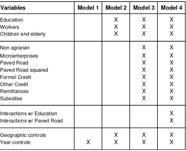
We consider four alternatives for estimating the model, which add explanatory

variables progressively (see Table A.3 for more detail):

Model 1: only time dummies

Model 2: adds basic educational and demographic characteristics and geographic

controls.

Model 3: adds other household economic characteristics

Model 4: adds several interactions between explanatory variables

A first step consisted in implementing the tests proposed by Bera et al. (2001) to

explore the presence of unobserved family random effects and serially correlated

the presence of both sources of persistence. We also estimated the linear dynamic model

and tested whether the non-linear restrictions implicit in the Lillard and Willis (1978) model are appropriate. The Wald tests do not provide evidence against this

simplification, though care must be taken given the possible low power of such

procedures. The results thus justify considering the joint presence of persistence due to

unmeasured, time invariant, family characteristics and serially correlated shocks.

Table 2: Tests for error components Bera et al. (2001)

statistic p-value statistic p-value statistic p-value statistic p-value

Individual Random Effect

LM (Var(u)=0) 147.45 0.0000 37.96 0.0000 19.77 0.0000 18.54 0.0000 ALM (Var(u)=0) 11.58 0.0007 39.1 0.0000 51.09 0.0000 50.11 0.0000 Serial Correlation

LM (rho=0) 423.37 0.0000 223.99 0.0000 180.53 0.0000 173.39 0.0000 ALM (rho=0) 287.51 0.0000 225.12 0.0000 211.85 0.0000 204.95 0.0000 Joint test

LM (Var(u)=0, rho=0) 434.96 0.0000 263.09 0.0000 231.62 0.0000 223.49 0.0000

Tests Model 1 Model 2 Model 3 Model 4

Source: Own estimates based on BASIS (1995-2001).

The relevance of the model adopted, that contemplates the presence of both

serial correlation and random effect is justified by the Bera et al´s tests and can be

appreciated graphically as follows. Figure 1 contains in circles the observed empirical correlations between yit and yi,t-s, for s= 0,1,2,3 periods. The graph also shows the

implicit correlation in a model with serial correlation and random effects (Model 4), the

solid line, with random effect but no serial correlation (the dashed line) and with serial

correlation but no random effects (marked with “x”). Clearly, and consistently with the

results of the Bera et al´s tests, the actual income correlations is better represented by a

Figure 1: Correlation structure of the income process in Rural El Salvador

0 0.25 0.5 0.75 1

0 1 2 3

Model 4 Actual

No autocorr. No RE

Source: Own estimates based on BASIS (1995-2001).

Table 3 presents estimates of the regression parameters of the autocorrelated

model together with the measures of the variance and persistence in incomes. In the

basic specification (Model 1), the time dummies explain only 0.030 of the total

variation in earnings. The estimated variance of the error components is 0.210, of which

0.069 corresponds to the variance of the family specific component and 0.140 to the

variance of the observation specific, serially correlated term. This latter variance is

simply the variance of the underlying white noise process (0.132) “inflated” by the first

order serial correlation coefficient (0.238). Hence, in the base model (no explanatory variables), differences in family specific (“permanent”) characteristics represent 33.1%

of the dispersion in incomes, which is much lower than the results obtained by Lillard

and Willis (73.1%) and others in the U.S. This is very likely due to the risky nature of

rural economic activities and the higher volatility of incomes in developing countries

like El Salvador. Hence, the stochastic variation of incomes over time is a key

Table 3: Sources of income persistence in Rural El Salvador

R2 _σ

u

2 _σ

µ2 σε2 συ2 ϕ λ ρ1

Drop in variance

Drop in individual

variance Obs.

(1) (2) (3) (4) (5) (6) (7) (8) (9) (10) (11) 1 0.030 0.210 0.069 0.132 0.140 0.238 0.331 0.490 1636 2 0.161 0.174 0.035 0.131 0.139 0.234 0.201 0.388 17.1% 49.6% 1636 3 0.240 0.153 0.024 0.123 0.129 0.214 0.157 0.337 26.9% 65.3% 1636 4 0.254 0.149 0.023 0.121 0.127 0.203 0.152 0.324 28.8% 67.3% 1636 No Autocorrelation _{0.272 0.134 0.012 0.123 0.123 0.000 0.087}

No Random Effects _{0.254 0.127 0.000 0.121 0.127 0.203 0.000} Model

Source: Own estimates based on BASIS (1995-2001).

Notes:(1) Overall R2, measures the explanatory performance of observed variables; (2) Overall variance of the error term; (3) Variance of the family specific term µ; (4) Variance of the white noise process ε; (5) Variance of the observation specific term υ; (6) Autocorrelation coefficient; (7) Proportion of total variance attributable to family component ((3)/(2)); (8) Adjacent correlation of error term; (9) Drop in overall variance (2) when explanatory variables are added; (10) Drop in family specific variance (3) when explanatory variables are added.

As expected, the addition of explanatory variables drops the overall error

variance. For example, when going from model 1 to 2, the addition of observed income

determinants makes the variance drop from .210 to .174, that is, 17% of the original

variance should be attributable now to measured family characteristics. A similar figure

for the family specific term is 49.3%: of the original family specific variance (0.069)

almost half can be explained by measured characteristics. This is remarkably similar to

the 44% obtained by Lillard and Willis.

Let us now turn to the analysis of sources of income persistence. The aggregate

adjacent correlation is 0.490, which gives a rough measure of overall persistence in

incomes. The autocorrelation coefficient is 0.238, which is a measure of the persistence

of the observation specific income shocks. Lillard and Willis obtained 0.840 and 0.406,

respectively, in their study. If the only source of persistence were the presence of

unobserved heterogeneity among families (no serial correlation), the adjacent

correlation would be 0.331 (just the ratio of family specific to total variance). From formula (6), 0.331 can be seen as an asymptotic limit of the correlations (the effect of

the “transitory” component vanishes), that is, in the longer term, after the effects of

shocks disappear, the correlation among any pair of periods is 0.331 for a given family.

It is important to clarify a distinction advanced in section 2. Going back to the

basic model with no explanatory variables, the idiosyncratic observation specific term

explaining differences in incomes, time and observation specific factors play the prime

role. Nevertheless, when we focus on income persistence, the adjacent correlation in the basic model is 0.49, of which 0.33 is due to the role played by time invariant-family

specific factors, being the rest attributable to the serially correlated observation specific

term. Therefore, when the interest lies on persistence, it is the family specific

components that play the key role. The importance of the idiosyncratic shock in

explaining income levels is reduced by the relatively low autocorrelation coefficient, as

it is clearly expressed in formula (6).

Note that when explanatory variables are deliberately omitted, their effect is

captured by each component of the error terms. When the Model 4 is considered, the

overall variance of the error term is reduced in around 28%, highlighting the role played

by observable factors. The family specific variance drops in around 63%, while the

variance of the idiosyncratic shock drops in only 10%, suggesting that the weight of

observable factors come from inherently family specific, relatively invariant

characteristics. The adjacent correlation of the error term drops to 0.324, meaning that

of the original 0.490, 33% of the persistence is related to the observable factors, 31.02%

to non-observed family specific terms and the rest to the persistence of shocks.

In sum, the results provide significant evidence that: (i) Volatility is the major

source of variation in incomes across rural families in El Salvador, much more so than

in developed countries. In any given year, the majority of variation in incomes is not

accounted for by education or observed family characteristics but instead is due to

transitory shocks; (ii) As far as the persistence of incomes over a lifetime, most (around

two-thirds) of the persistency in low and high income states is due to idiosyncratic

differences between families related to endowments, including unobserved income determinants (unobserved heterogeneity). The persistence of bad shocks is of second

order given that the correlation of bad shocks is relatively low (0.24) in these data. So

over a lifetime transitory components average out.

As a result, low incomes at any given time in rural El Salvador are strong

predictors of low incomes later in life, even controlling for observed family characteristics. In other words, while a large proportion of total cross-section inequality

(as measured by the variance of logarithmic incomes) is explained by income

instability, life-cycle inequality is largely due to the permanent income component,

particularly to relatively time-invariant productive characteristics of families and their

members. The latter seem then to be more likely candidate for the existence of poverty

6 Poverty dynamics

The previous section explored the sources of persistence in household incomes. The

results can be used to quantify the impact of the different factors in relevant features of

the distribution of incomes, in particular the proportion of poor households. This section

presents results of a simple exercise, with the goal of studying the effects of negative

shocks on the poverty status of particular groups. We consider two extensions.

First, as advanced in previous work, in particular Rodríguez-Meza and

González-Vega (2004), the distinction between agrarian and non-agrarian households is

a key element since the latter group is more diversified. These groups of households

likely obey structurally different income patterns so it is worth exploring their dynamics

separately. Thus, we divide the sample in “non-agrarian” and “agrarian” based on the

activities that families dedicate most of their work hours and estimated the AR(1)

model. Income persistence measures are shown in Table 4 (see basic regression results

in Table A.4).

A first relevant result is that the variance of the family error component is now

slightly negative. Following Maddala and Mount (1973) this can be prudently

interpreted as suggesting zero variances (See Baltagi 2001, pp. 19 for a discussion). One

interpretation of this finding is that the income variation in the overall sample can be

appropriately summarized by the “agrarian vs. non-agrarian” status, and hence, family

income persistence may be arising from high income persistence in one of these groups.

In such case the only source of persistence is now due to the serially correlated

idiosyncratic error term. In fact, as shown in Table 4, the stochastic term for agrarian households explain a larger fraction of income variation and is also more persistent, as

can be appreciated from the estimated autocorrelation coefficients (0.207 compared

with 0.161 for non-agrarian households). This suggests that agrarian households are

more exposed to more persistent shocks in light of having less diversified income

Table 4. Variance components and persistence, Agrarian and Non-agrarian Households

R2 Prais-Winsten transf. model

R2 pooled OLS σu

2 _σ

µ2 σε2 συ2 ϕ λ Obs.*

Agrarian 0.124 0.137 0.161 0.000 0.154 0.161 0.207 0 969

Non agrarian 0.354 0.375 0.060 0.000 0.059 0.060 0.161 0 667

Source: Own estimates based on BASIS (1995-2001).

* Non balanced panel. Households move from agrarian to non-agrarian activities (See Rodríguez-Meza et al. (2004)). Total agrarian households in estimation sample are 265 in 1995, 250 in 1997, 240 in 1999, and 214 in 2001

Second, based on the previous estimates we implemented simple simulations of the

effect of a large negative shock on poverty dynamics. The exercise is implemented for

agrarian and non-agrarian households with low, median and high education, located

close to a paved road or far from it. We started by defining a focus household defined by a particular level of the observed explanatory variables (Table A.5 reports the values

of the variables set for the simulations). This defines representative households in the

two sectors (agrarian, non-agrarian), three levels of education (low, median, high), and

two alternative distances to a paved road (close, far). For each of these twelve groups

we predicted steady state income distributions as:

yit = xit´ + µi + vit

using the estimated parameters (pooled OLS) and _⎟⎟

⎠ ⎞ ⎜⎜ ⎝ ⎛ ∼ − 2 1 2 , 0 ρ ε σ

ν_it N . That is, for a given

value of x, the income of a hypothetical household is generated by computing its

predicted long-term income potential as judged by its measured endowments and a

random draw from the implied long run distribution of the idiosyncratic error term vit

parameterized as Gaussian.8 For this empirical distribution we have computed measures of moderate and extreme poverty rates. These figures appear in the last line of each

panel of Table 5 under the SS (steady state) row. For example, the moderate poverty

rate for typical agrarian households located close to a paved road and with low

education is 0.491. Of course, within each particular group it is the idiosyncratic error

term what varies from household to household. The “steady state” distribution refers to

the unconditional, long-run distribution of vit as implied by the AR(1) structure, and is

8

to be interpreted as the prevalent distribution after all dynamic adjustments have taken

place.

Next we introduced a drastic shock where we shifted the empirical distributions

of log-incomes by a negative factor (the first percentile of the distribution of steady state

νit). The resulting poverty rates are shown in the first line of each panel of Table 5. For

example, for agrarian, low-educated households located close to a paved road, poverty

incidence jumps from 0.491 to 0.992. Then we predicted incomes for subsequent

periods by using the estimated AR(1) structure, computing poverty in each two-year

period. Given that the process is stationary, poverty figures should revert back to their

long-run levels. As it turns out, it takes approximately 5 periods (approximately 10

years) for low educated, agrarian households to see their poverty rates recovered to their

original steady state levels. As expected, the speed of recovery for observationally

similar non-agrarian households is much faster. For example, households with low

education start with poverty rates above 90% after the shock, in the first period poverty

drops to about 70% in the agrarian group and to less than 30% for the more diversified,

non-agrarian households. The nature of this particular exercise is rather drastic, and is meant to be suggestive of differences in poverty dynamics in the aftermath of an income

shock.

Figure 2 allows us to explore the effects on poverty paths of changes in

education and distance to a paved road. An increase in the educational level (percentile

25 to percentile 90) reduces steady state poverty in about 10 percentage points and increases the speed of recovery both for agrarian and non-agrarian households.

Reducing the distance to a paved road from 8 to 1 km has also a strong negative effect

on poverty for agrarian households. For non-agrarian households, reducing the distance

from percentile 75 to 25 (from 5 to ½ km) has a smaller effect (less than 2 points). In

both cases the interaction between distance to paved road and education has a smaller,

Table 5. Simulated Poverty Rates, Agrarian and Non-agrarian Households

Households close to a paved road

0 0.992 0.992 0.986 0.908 0.874 0.781 2 0.676 0.654 0.621 0.261 0.212 0.114 4 0.530 0.508 0.478 0.160 0.126 0.061 6 0.500 0.484 0.450 0.148 0.110 0.057 8 0.492 0.478 0.443 0.146 0.110 0.055 10 0.491 0.478 0.443 0.145 0.109 0.055 12 0.491 0.477 0.442 0.145 0.109 0.055 14 0.491 0.477 0.442 0.145 0.109 0.055 16 0.491 0.477 0.442 0.145 0.109 0.055 18 0.491 0.477 0.442 0.145 0.109 0.055 SS 0.491 0.477 0.442 0.145 0.109 0.055

0 0.974 0.971 0.965 0.730 0.684 0.546 2 0.514 0.498 0.466 0.078 0.059 0.029 4 0.377 0.360 0.321 0.043 0.033 0.014 6 0.353 0.323 0.292 0.038 0.029 0.012 8 0.345 0.321 0.285 0.037 0.029 0.011 10 0.344 0.320 0.285 0.037 0.029 0.011 12 0.344 0.320 0.285 0.037 0.029 0.011 14 0.344 0.320 0.285 0.037 0.029 0.011 16 0.344 0.320 0.285 0.037 0.029 0.011 18 0.344 0.320 0.285 0.037 0.029 0.011 SS 0.344 0.32 0.285 0.037 0.029 0.011

low median

Extreme Poverty in year

high Non agrarian with education

low median high Agrarian with education Moderate Poverty

in year

Households far from a paved road

0 0.994 0.993 0.990 0.916 0.882 0.753 2 0.740 0.700 0.639 0.289 0.220 0.091 4 0.609 0.569 0.489 0.179 0.128 0.051 6 0.583 0.534 0.462 0.167 0.118 0.046 8 0.577 0.527 0.457 0.165 0.116 0.044 10 0.575 0.525 0.456 0.163 0.115 0.043 12 0.575 0.525 0.456 0.163 0.115 0.043 14 0.575 0.525 0.456 0.162 0.115 0.043 16 0.575 0.525 0.456 0.162 0.115 0.043 18 0.575 0.525 0.456 0.162 0.115 0.043 SS 0.575 0.525 0.456 0.162 0.115 0.043

0 0.985 0.980 0.970 0.757 0.687 0.508 2 0.601 0.548 0.480 0.092 0.062 0.024 4 0.456 0.412 0.338 0.051 0.035 0.011 6 0.426 0.384 0.304 0.046 0.030 0.011 8 0.418 0.375 0.297 0.046 0.029 0.011 10 0.416 0.374 0.296 0.045 0.029 0.011 12 0.415 0.374 0.296 0.045 0.029 0.011 14 0.415 0.374 0.296 0.045 0.029 0.011 16 0.415 0.374 0.296 0.045 0.029 0.011 18 0.415 0.374 0.296 0.045 0.029 0.011 SS 0.415 0.374 0.296 0.045 0.029 0.011 Extreme Poverty

in year

Agrarian with education Non agrarian with education Moderate Poverty

in year low median high low median high

Source: Own estimates based on BASIS (1995-2001).

Figure 2. Simulated effects on poverty rates of changes in education

and distance to a paved

Source: Own estimates based on BASIS (1995-2001).

7 Conclusions

We use a unique panel dataset (1995-2001) of rural El Salvador to investigate the main

sources of the persistence and variability of incomes. The paper investigates the extent

to which families are continuously poor due to endowments (observed and unobserved)

that yield low income potential or due to systematic income shocks that they are unable

to smooth. We follow the approach that was first pioneered by Lillard and Willis (1978)

to study income mobility in the U.S. who main appealing features has withstood

scrutiny in subsequent studies. We implement testing procedures proposed by Bera,

Yoon and Sosa Escudero (2001) robust test for presence of unobserved heterogeneity, state dependence or both based on a 'null' model of no persistency, and find evidence

supporting the validity of the Lillard and Willis (1978) basic model specification.

Our main results are that being persistently low income or poor in rural El

Salvador is largely a result of starting and continuing with unfavorable endowments or

characteristics and to some extent to past “bad luck”. Observed income determinants

account for about half of this income persistence. Controlling for unobserved heterogeneity leaves little room for pure state dependence. The analysis indicates that

some of the main culprits are manipulable by policy interventions, although many not in

the short term. For example, investments in rural roads can facilitate the diversification

Agrarian Households 0% 10% 20% 30% 40% 50% 60% 70% 80% 90% 100%

0 2 4 6 8 10 12 14 16 18 SS

years po v e rt y Non-Agrarian Households 0% 10% 20% 30% 40% 50% 60% 70% 80% 90% 100%

0 2 4 6 8 10 12 14 16 18 SS

years po v e rt y

of families from subsistence agriculture to more dynamic agricultural or off-farm

activities in a relatively short span. However, education is a chief source of attraction to low income states since it can take one or two decades for a family to break the

intergenerational transmission of low education. In further extensions of this work we

plan to further quantify the role of these measured factors and their interactions in the

References

Abowd, J., and D. Card 1989. "On the Covariance Structure of Earnings and Hours

Changes," Econometrica, 57, 411–445.

Antman, F. and D. Mckenzie. 2005. “Poverty traps and non-linear dynamics with

measurement error and individual heterogeneity”, mimeo, Stanford University.

Anderson, T. and C. Hsiao. 1982. “Estimation of dynamic models with

error-components”, Journal of Econometrics, 18, 47-82.

Arellano, M. 2003. Panel Data Econometrics, Oxford University Press, Oxford.

Arellano, M. and S. Bond. 1991. “Some specification tests for panel data: Monte Carlo

evidence and an application to employment equations”, Review of Economic

Studies, 58, 277-297.

Azariadis, C., and J. Stachurski. 2005. “Poverty Traps.” In Handbook of Economic

Growth, ed. P. Aghion and S. Durlauf. North Holland. 204

Baltagi, B. 2001. Econometric Analysis of Panel Data, Wiley, New York.

Beneke de Sanfeliu, M., and M. Shi. 2004. “Dinámica del Ingreso en El Salvador.”

Serie de Investigación 2. Antiguo Cuscatlán: Departamento de Estudios

Económicos y Sociales (DEES)/FUSADES.

Bera, A., W. Sosa Escudero, and M. Yoon. 2001. “Tests for the error component model

under local misspecification”, Journal of Econometrics, 101, 1-23.

Blanchard, O., and L. Katz. 1992. “Regional Evolutions.” Brookings Papers on

Economic Activity, 32, 159-85.

Chaudhuri, S. 2000. “Empirical Methods for Assessing Household Vulnerability to

Poverty.” School of International and Public Affairs, Columbia University, New

York.

Chaudhuri, S., J. Jalan, and A. Suryahadi. 2002. “Assessing Household Vulnerability to

Poverty: A Methodology and Estimates for Indonesia.” Department of Economics

Discussion Paper 0102-52, Columbia University, New York.

Fields, G., R. Duval, S. Freije, and M. Puerta. 2005. “Earnings Mobility in Argentina,

Mexico, and Venezuela: Testing the Divergence of Earnings and the Symmetry of

Mobility Hypotheses.” Unpublished paper, Cornell University, Ithaca, NY.

Freije, S., and A. Souza. 2002. “Earnings Dynamics and Inequality in Venezuela: 1995–

1997.” Working Paper 0211, Vanderbilt University, Department of Economics,

Friedman, M. 1962. “Capitalism and Freedom.” Princeton, NJ: Princeton University.

Friedman, M. and S. Kuznets. 1954. “Incomes from Independent Professional Practice.”

National Bureau of Economic Research, New York (1945), 1954.

Galiani, S., C. Lamarche, A. Porto, and W. Sosa Escudero. 2005. “Persistence and

Regional Disparities in Unemployment: Argentina 1980-1981”, Regional Science

and Urban Economics, 35, 375-394.

Geweke, J., and M. Keane. 2000. “An Empirical Analysis of Income Dynamics among

Men in the PSID: 1968–1989.” Journal of Econometrics 96: 293–356.

Gottschalk, P., and R.A. Moffitt. 1994. "Welfare Dependence: Concepts, Measures, and

Trends," American Economic Review. American Economic Association, vol.

84(2), pages 38-42, May.

Hendry, D.F. and G.E. Mizon. 1978. “Serial correlation as a convenient simplification,

not a nuisance: A comment on a study of the demand for money by the Bank of

England”, Economic Journal, 88, 549-563.

Holtz-Eakin, D. 1988. “Testing for individual effects in autorregresive models”, Journal

of Econometrics, 39, 297-307.

Horowitz J.L. and M. Markatou. 1996. “Semiparametric estimation of regression

models for panel data”, Review of Economic Studies 63, 145-168.

Jalan, J., and M. Ravallion. 1999. “Income Gains to the Poor from Workfare: Estimates

for Argentina’s Trabajar Program.” Policy Research Working Paper 2149, World

Bank, Washington, DC.

Jimenez-Martin, S. 1998. “On the testing of heterogeneity effects in dynamic

unbalanced panel data models”, Economic Letters, 58, 157-163.

Judson, R. and A. Owen. 1999. “Estimating dynamic panel data models: a guide for

macroeconomists”, Economic Letters, 65, 9-15.

Lanjouw, P. 2001. “Nonfarm Employment and Poverty in Rural El Salvador.” World

Development 29 (3): 529–47.

Lillard, L. and R. Willis. 1978. “Dynamic aspects of earning mobility”, Econometrica,

46, 985-1012.

MaCurdy, T. 1982. “The use of time series processes to model the error structure of

Maddala, G.S. and T. Mount. 1973. “A comparative study of alternative estimators for

variance components models used in econometric applications”, Journal of the

American Statistical Association, 68, 324-328.

McCall, J.J. 1973. Income Mobility, Racial Discrimination, and Economic Growth.

Lexington Books, Lexington, MA. Redner, R.A., Walker, H.F., 1984.

Meghir, C. and L. Pistaferri. 2002. "Income Variance Dynamics and Heterogeneity,"

CEPR Discussion Papers 3632, C.E.P.R. Discussion Papers.

Newhouse, D. 2005. “The Persistence of Income Shocks: Evidence from Rural

Indonesia”, Review of Development Economics 9 (3), 415-433.

Pritchett, L., A. Suryahadi, and S. Sumarto. 2000. “Quantifying Vulnerability to

Poverty. A Proposed Measure Applied to Indonesia.” Policy Research Working

Paper 2437, World Bank, Washington, DC.

Ravallion, M., and S. Chaudhuri. 1997. “Risk and Insurance in Village India: A

Comment.” Econometrica 65 (1): 171–84.

Ravallion, M. and M. Lokshin, 2004. “Household Income Dynamics in Two Transition

Economies.” Studies in Nonlinear Dynamics & Econometrics, Berkeley

Electronic Press, vol. 8 (3)

Rodríguez-Meza, J., and C. González-Vega. 2004. “Household Income Dynamics and Poverty Traps in El Salvador.” Paper written for AAEA (American Agriculture

Economists Association) annual meeting, Ohio State University, Columbus.

Tannuri-Pianto, M., D. Pianto, O. Arias, and M. Beneke de Sanfeliu. 2005.

“Determinants and Returns to Productive Diversification in Rural El Salvador.”

Background paper for the Beyond the City: The Rural Contribution to

Development, World Bank, Washington, DC.

Welch, F. 1999. In defense of inequality, American Economic Review, Papers and

Proceedings, May.

World Bank. 2005. “El Salvador Poverty Assessment: Strengthening Social Policy.”

Report 29594-SV. World Bank, Washington, DC.

Zincenko, F. 2005. “The power of panel tests for serial correlation under dynamic

Appendix

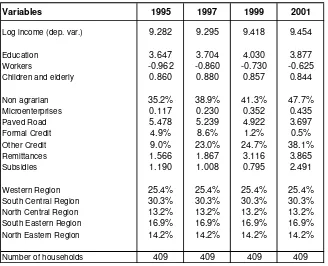
Table A.1. Definition of variables

Variables Definition

Log income (dep. var.) Log of per capita household income

Education Average years of education of members in the labor force (imputed) Workers Log of workers per capita

Children and elderly Log of number of children and elderly

Non agrarian =1 if main household activity is non agricultural Microenterprises Number of microenterprises

Paved Road Distance to paved road (in km) Formal Credit =1 if household received formal credit Other Credit =1 if household received other credit Remittances Log of remittances

Subsidies Log of subsidies from the Government

Interactions w/ Education and Formal Credit, Other Credit, Remittances and Subsidies

Interactions w/ Paved Road and Formal Credit, Other Credit, Remittances, Subsidies and Education

Geographic controls Region reported in the first interview (West, South Central, North Central, South Eastern and North Eastern)

Table A.2. Descriptive statistics in Estimation Sample

Variables 1995 1997 1999 2001

Log income (dep. var.) 9.282 9.295 9.418 9.454

Education 3.647 3.704 4.030 3.877

Workers -0.962 -0.860 -0.730 -0.625

Children and elderly 0.860 0.880 0.857 0.844

Non agrarian 35.2% 38.9% 41.3% 47.7%

Microenterprises 0.117 0.230 0.352 0.435

Paved Road 5.478 5.239 4.922 3.697

Formal Credit 4.9% 8.6% 1.2% 0.5%

Other Credit 9.0% 23.0% 24.7% 38.1%

Remittances 1.566 1.867 3.116 3.865

Subsidies 1.190 1.008 0.795 2.491

Western Region 25.4% 25.4% 25.4% 25.4%

South Central Region 30.3% 30.3% 30.3% 30.3%

North Central Region 13.2% 13.2% 13.2% 13.2%

South Eastern Region 16.9% 16.9% 16.9% 16.9%

North Eastern Region 14.2% 14.2% 14.2% 14.2%

Table A.3. Alternative models.

Variables Model 1 Model 2 Model 3 Model 4

Education X X X

Workers X X X

Children and elderly X X X

Non agrarian X X

Microenterprises X X

Paved Road X X

Paved Road squared X X

Formal Credit X X

Other Credit X X

Remittances X X

Subsidies X X

Interactions w/ Education X

Interactions w/ Paved Road X

Geographic controls X X X

Table A.4. Regression results

Dependent variable: Log of per capita household income Pooled OLS estimates

Agrarian Non agrarian

Education 0.002 0.015

(0.21) (2.40)*

Workers 0.118 0.149

(3.93)** (5.96)**

Children and elderly -0.053 -0.122

(2.07)* (5.53)**

Microenterprises 0.064 0.073

(1.70) (4.31)**

Paved Road -0.021 -0.010

(3.57)** (1.48)

Paved Road squared 0.001 0.000

(2.91)** (0.98)

Formal Credit 0.060 -0.023

(0.40) (0.18)

Other Credit -0.080 -0.119

(1.24) (2.14)*

Remittances -0.025 0.000

(4.12)** (0.01)

Subsidies -0.009 -0.019

(0.92) (2.24)*

Formal Credit 0.038 0.017

(1.37) (1.08)

Other Credit 0.021 0.025

(1.57) (2.70)**

Remittances 0.003 0.001

(2.15)* (1.07)

Subsidies -0.000 0.001

Interactions w/ Education

(0.23) (0.84)

Formal Credit -0.018 -0.002

(1.23) (0.27)

Other Credit 0.000 -0.000

(0.03) (0.05)

Remittances 0.001 0.000

(2.30)* (0.44)

Subsidies 0.000 0.001

(0.05) (0.92)

Education 0.002 0.002

Interactions w/ Paved Road

(2.00)* (2.17)*

Constant 9.401 9.586

(158.60)** (179.37)**

Observations 969 667

R-squared 0.14 0.38

Table A.5. Values used in the simulations

Variables Agrarian Non-agrarian

Education

low (percentile 25) 1.00 2.67

median (percentile 50) 3.00 4.50

high (percentile 90) 6.60 9.00

Paved Road

close (percentile 25) 1.00 0.40

far (percentile 75) 8.00 5.00

Workers (mean) -0.77 -0.83

Children and elderly (mean) 0.87 0.85

Microenterprises (mean) 0.13 0.51

Formal Credit (min) 0 0

Other Credit (min) 0 0

Remittances (mean) 2.80 2.32

Subsidies (mean) 1.38 1.36

Western Region (other regions = 0) 1 1

SERIE DOCUMENTOS DE TRABAJO DEL CEDLAS

Todos los Documentos de Trabajo del CEDLAS están disponibles en formato electrónico en <www.depeco.econo.unlp.edu.ar/cedlas>.

• Nro. 37 (Junio, 2006). Walter Sosa-Escudero, Mariana Marchionni y Omar Arias. "Sources of Income Persistence: Evidence from Rural El Salvador".

• Nro. 36 (Mayo, 2006). Javier Alejo. "Desigualdad Salarial en el Gran Buenos Aires: Una Aplicación de Regresión por Cuantiles en Microdescomposiciones".

• Nro. 35 (Abril, 2006). Jerónimo Carballo y María Bongiorno. "La Evolución de la Pobreza en Argentina: Crónica, Transitoria, Diferencias Regionales y Determinantes (1995-2003)".

• Nro. 34 (Marzo, 2006). Francisco Haimovich, Hernán Winkler y Leonardo Gasparini. "Distribución del Ingreso en América Latina: Explorando las Diferencias entre Países".

• Nro. 33 (Febrero, 2006). Nicolás Parlamento y Ernesto Salinardi. "Explicando los Cambios en la Desigualdad: Son Estadísticamente Significativas las Microsimulaciones? Una Aplicación para el Gran Buenos Aires".

• Nro. 32 (Enero, 2006). Rodrigo González. "Distribución de la Prima Salarial del Sector Público en Argentina".

• Nro. 31 (Enero, 2006). Luis Casanova. "Análisis estático y dinámico de la pobreza en Argentina: Evidencia Empírica para el Periodo 1998-2002".

• Nro. 30 (Diciembre, 2005). Leonardo Gasparini, Federico Gutiérrez y Leopoldo Tornarolli. "Growth and Income Poverty in Latin America and the Caribbean: Evidence from Household Surveys".

• Nro. 29 (Noviembre, 2005). Mariana Marchionni. "Labor Participation and Earnings for Young Women in Argentina".

• Nro. 28 (Octubre, 2005). Martín Tetaz. "Educación y Mercado de Trabajo".

• Nro. 27 (Septiembre, 2005). Matías Busso, Martín Cicowiez y Leonardo Gasparini. "Ethnicity and the Millennium Development Goals in Latin America and the Caribbean".

• Nro. 26 (Agosto, 2005). Hernán Winkler. "Monitoring the Socio-Economic Conditions in Uruguay".

• Nro. 24 (Junio, 2005). Francisco Haimovich y Hernán Winkler. "Pobreza Rural y Urbana en Argentina: Un Análisis de Descomposiciones".

• Nro. 23 (Mayo, 2005). Leonardo Gasparini y Martín Cicowiez. "Equality of Opportunity and Optimal Cash and In-Kind Policies".

• Nro. 22 (Abril, 2005). Leonardo Gasparini y Santiago Pinto. "Equality of Opportunity and Optimal Cash and In-Kind Policies".

• Nro. 21 (Abril, 2005). Matías Busso, Federico Cerimedo y Martín Cicowiez. "Pobreza, Crecimiento y Desigualdad: Descifrando la Última Década en Argentina".

• Nro. 20 (Marzo, 2005). Georgina Pizzolitto. "Poverty and Inequality in Chile: Methodological Issues and a Literature Review".

• Nro. 19 (Marzo, 2005). Paula Giovagnoli, Georgina Pizzolitto y Julieta Trías. "Monitoring the Socio-Economic Conditions in Chile".

• Nro. 18 (Febrero, 2005). Leonardo Gasparini. "Assessing Benefit-Incidence Results Using Decompositions: The Case of Health Policy in Argentina".

• Nro. 17 (Enero, 2005). Leonardo Gasparini. "Protección Social y Empleo en América Latina: Estudio sobre la Base de Encuestas de Hogares".

• Nro. 16 (Diciembre, 2004). Evelyn Vezza. "Poder de Mercado en las Profesiones Autorreguladas: El Desempeño Médico en Argentina".

• Nro. 15 (Noviembre, 2004). Matías Horenstein y Sergio Olivieri. "Polarización del Ingreso en la Argentina: Teoría y Aplicación de la Polarización Pura del Ingreso".

• Nro. 14 (Octubre, 2004). Leonardo Gasparini y Walter Sosa Escudero. "Implicit Rents from Own-Housing and Income Distribution: Econometric Estimates for Greater Buenos Aires".

• Nro. 13 (Septiembre, 2004). Monserrat Bustelo. "Caracterización de los Cambios en la Desigualdad y la Pobreza en Argentina Haciendo Uso de Técnicas de Descomposiciones Microeconometricas (1992-2001)".

• Nro. 12 (Agosto, 2004). Leonardo Gasparini, Martín Cicowiez, Federico Gutiérrez y Mariana Marchionni. "Simulating Income Distribution Changes in Bolivia: a Microeconometric Approach".

• Nro. 11 (Julio, 2004). Federico H. Gutierrez. "Dinámica Salarial y Ocupacional: Análisis de Panel para Argentina 1998-2002".

• Nro. 10 (Junio, 2004). María Victoria Fazio. "Incidencia de las Horas Trabajadas en el Rendimiento Académico de Estudiantes Universitarios Argentinos".

• Nro. 8 (Abril, 2004). Federico Cerimedo. "Duración del Desempleo y Ciclo Económico en la Argentina".

• Nro. 7 (Marzo, 2004). Monserrat Bustelo y Leonardo Lucchetti. "La Pobreza en Argentina: Perfil, Evolución y Determinantes Profundos (1996, 1998 Y 2001)".

• Nro. 6 (Febrero, 2004). Hernán Winkler. "Estructura de Edades de la Fuerza Laboral y Distribución del Ingreso: Un Análisis Empírico para la Argentina".

• Nro. 5 (Enero, 2004). Pablo Acosta y Leonardo Gasparini. "Capital Accumulation, Trade Liberalization and Rising Wage Inequality: The Case of Argentina".

• Nro. 4 (Diciembre, 2003). Mariana Marchionni y Leonardo Gasparini. "Tracing Out the Effects of Demographic Changes on the Income Distribution. The Case of Greater Buenos Aires".

• Nro. 3 (Noviembre, 2003). Martín Cicowiez. "Comercio y Desigualdad Salarial en Argentina: Un Enfoque de Equilibrio General Computado".

• Nro. 2 (Octubre, 2003). Leonardo Gasparini. "Income Inequality in Latin America and the Caribbean: Evidence from Household Surveys".