Analysis of power distribution systems using a multicore environment

(1)

PhD Thesis

Analysis of Power Distribution Systems

Using a Multicore Environment

Luis Gerardo Guerra Sánchez

(2)

(3)

Analysis of Power Distribution Systems

Using a Multicore Environment

Luis Gerardo Guerra Sánchez

Dissertation submitted to the Doctorate Office

of the Universitat Politècnica de Catalunya in

partial fulfillment of the requirements for the

degree of Doctor of Philosophy by the

UNIVERSIDAD DE MALAGA

UNIVERSIDAD DE SEVILLA

UNIVERSIDAD DEL PAÍS VASCO/EUSKAL ERRIKO UNIBERTSITATEA

UNIVERSITAT POLITÈCNICA DE CATALUNYA

Joint Doctoral Programme in

Electric Energy Systems

(4)

Printed by the UPC Barcelona, March 2016 ISBN: --

Research Project: --

UNIVERSITAT POLITÈCNICA DE CATALUNYA Escola de Doctorat

Edifici Vertex. Pl. Eusebi Güell, 6 08034 Barcelona

Web: http://www.upc.edu UNIVERSIDAD DE MALAGA Escuela de Doctorado

Pabellón de Gobierno - Plaza el Ejido s/n (29013) Málaga.

Web: http://www.uma.es UNIVERSIDAD DE SEVILLA Escuela Internacional de Doctorado

Pabellón de México - Paseo de las Delicias, s/n 41013 Sevilla

Web: http://www.us.es

UNIVERSIDAD DEL PAÍS VASCO/EUSKAL ERRIKO UNIBERTSITATEA Escuela de Master y Doctorado

(5)

(6)

(7)

Acknowledgments

I have never been a good writer; I always related more to numbers and equations than I ever did to words, which is probably why I became an engineer. However, as I finish this chapter of my life, I would like to take a moment to express my appreciation and gratitude towards everyone who has helped or supported me in any way during this time.

I have always seen myself as a man of faith and this faith has been one of the main driving forces in my adult life. The comfort and solace I find in God has given me the strength to pursue my goals and the peace of mind to overcome difficult times; His love makes everything possible.

The completion of this Thesis has required an enormous amount of work and effort from my part; however none of it would have been possible without the support and guidance from Professor Juan Antonio Martínez Velasco. It has been a real pleasure and honor to work with someone so dedicated and committed to his work. I am truly grateful to him for giving me the opportunity to pursue this path and prove myself.

I would also like to thank those whose help has directly contributed to the development of my work, Víctor Fuses, Gabriel Verdejo, and everybody at RDLab. Víctor’s help was invaluable during the early stages when we were trying to acquire our own computer cluster and RDLab provided the much needed technical support to set it up. Their hard work is one of the reasons behind this Thesis’ success.

I cannot see myself being here without my family; I have been blessed with the unconditional love and support of my parents, Mauricio and Betty. They have always encouraged me to be the best person I can be and to look for new horizons; words fail me to express the gratitude and love I feel for them. Many people go through their lives without really getting to know their siblings, to them they are just strangers who live in the same house; to me Carlos is not only my brother, he is my best friend and I am really thankful for having him in my life. Of course I cannot forget my sister-in-law Samantha, who soon will bless us with the greatest gift of all, my soon-to-be-born nephew Carlos Fernando.

For a long time my life revolved primarily around my work and I couldn’t help feeling that something was missing; that emptiness was filled when a very special person entered my life, my girlfriend Canan. Her love has been a constant source of inspiration and I can only hope to be there for her as she has been there for me; the uncertainties of the future do not scare me if she is with me.

(8)

Torres, Javier Portillo, Violeta Pastore, Javier Saade, René González, Walter Leiva, Laura Di Raimondo, Alejandra García, Jorge Acevedo, Alberto Canales, and Manolo López.

Finally, as I embark myself on a new adventure, I cannot help but to feel excited about what is to come; for I know this is not the beginning of the end but the end of the beginning.

(9)

“It’s a magical world, Hobbes, ol’ buddy, Let’s go exploring!”

(10)

(11)

List of Publications

Journal Publications:

J.A. Martinez and G. Guerra, “A Parallel Monte Carlo method for optimum allocation of distributed generation,” IEEE Trans. on Power Systems, vol. 29, no. 6, pp. 2926-2933, November 2014.

J.A. Martinez and G. Guerra, “A Parallel Monte Carlo approach for distribution reliability assessment”, IET Gener., Transm. Distrib., vol. 8, no. 11, pp. 1810-1819, November 2014.

J.A. Martinez-Velasco and G. Guerra, “Analysis of large distribution networks with distributed energy resources”, Ingeniare, vol. 23, no. 4, pp. 594-608, October 2015.

G. Guerra and J.A. Martinez, “Optimum allocation of distributed generation in multi-feeder systems using long term evaluation and assuming voltage-dependent loads,”

Sustainable Energy, Grids and Networks, vol. 5, pp. 13-26, March 2016.

J.A. Martinez and G. Guerra, “Reliability Assessment of Distribution Systems with Distributed Generation Using a Power Flow Simulator and a Parallel Monte Carlo Approach,” Submitted for publication in Sustainable Energy, Grids and Networks.

Conference Publications:

J.A. Martinez and G. Guerra, “Optimum placement of distributed generation in three-phase distribution systems with time varying load using a Monte Carlo approach,” IEEE

PES General Meeting, San Diego, July 2012.

J.A. Martinez and G. Guerra, “A Monte Carlo approach for distribution reliability assessment considering time varying loads and system reconfiguration,” IEEE PES

General Meeting, Vancouver, July 2013.

G. Guerra and J.A. Martinez, “A Monte Carlo method for optimum placement of photovoltaic generation using a multicore computing environment,” IEEE PES General

Meeting, National Harbor, USA, July 2014.

G. Guerra, J.A. Corea-Araujo, J.A. Martinez, and F. Gonzalez-Molina, “Generation of bifurcation diagrams for ferroresonance characterization using parallel computing,”

(12)

Book Chapters:

J.A. Martinez-Velasco and G. Guerra, “Allocation of Distributed Generation for Maximum Reduction of Energy Losses in Distribution Systems,” Chapter 12 of Energy

(13)

List of Tables

Table 2.1. Task-function input variables. 42

Table 2.2. Simulation times comparison. 45

Table 3.1. Range of optimization parameter variability. 61

Table 3.2. Summary of solar and wind resources. 66

Table 4.1. Optimum allocation of two capacitor banks - 100 nodes. 82

Table 4.2. Optimum allocation of one capacitor bank with time varying load - 100 nodes.

83

Table 4.3. Optimum allocation of one generation unit - 100 nodes. 84

Table 4.4. Optimum allocation of generation units - 100 nodes. 85

Table 4.5. Optimum allocation of generation units – theoretical results in snapshot mode – 100 nodes.

85

Table 4.6. Optimum allocation of generation units - 500 nodes. 86

Table 4.7. Summary of solar and wind resources. 87

Table 4.8. Optimum allocation of PV generation units. 89

Table 4.9. Optimum allocation of wind generation units. 90

Table 4.10. Simulation results using multicore computing. 91

Table 4.11. Simulation results using a refined Monte Carlo method – 500-node test system.

95

Table 4.12. Simulation results using a refined Monte Carlo method – 1000-node test system – PV generation.

96

Table 4.13. Simulation results using a refined Monte Carlo method – 1000-node test system – Wind generation.

97

Table 4.14. Test system information. 98

Table 4.15. Summary of solar resources. 98

Table 4.16. Short term evaluation (1 year) – Energy losses without distributed generation.

99

Table 4.17. Short term evaluation (1 year) – Optimum allocation of PV generation units (constant power).

100

Table 4.18. Short term evaluation (1 year) – Comparison of simulation results - Constant Power Load Model - 60 cores.

101

Table 4.19. Short term evaluation (1 year) – Comparison of simulation results - Constant Impedance Model - 60 cores.

101

Table 4.20. Short term evaluation (1 year) – Comparison of simulation results - ZIP Model - 60 cores.

102

Table 4.21. Short term evaluation (1 year) – Energy loss reduction – Conventional Monte Carlo method.

(18)

[image:18.595.65.478.79.766.2]

Table 4.22. Scenario for long term evaluation. 104

Table 4.23. Long Term Evaluation (17 years) – Energy losses without distributed generation.

104

Table 4.24. Long Term Evaluation – Comparison of simulation results. 105

Table 4.25. Long Term Evaluation – Total generation and energy loss reduction.

105

Table 4.26. Short Term Evaluation (1 year) – Additional reduction of energy losses.

111

Table 4.27. Long Term Evaluation – Percentage reduction of energy losses (%).

112

Table 4.28. Long Term Evaluation – “Divide and Conquer” procedure. 113

Table 4.29. Long Term Evaluation – Summary of results with “Divide and Conquer” procedure.

113

Table 5.1. Summary of solar resources. 131

Table 5.2. Characteristics of protective devices. 131

Table 5.3. Interconnection protection of PV plants. 132

Table 5.4. Failure statistics for overhead line sections. 133

Table 5.5. Failure statistics for system elements. 133

Table 5.6. Reliability indices - Sensitivity study. 141

Table 5.7. Probability distributions of reliability indices – Without DG – 420 runs.

141

Table 5.8. Probability distributions of reliability indices – With DG 142

Table 5.9. Probability distributions of reliability indices – With DG (DG equipment can fail) – 420 runs.

142

Table 5.10. Simulation times – Scenario 3. 142

Table 5.11. Reliability indices without switching operations (Scenario 3) – With Distributed generation (DG equipment can fail) – 1 Run.

145

Table 5.12. Simulation times – With Distributed generation (DG equipment can fail) – Scenario 3.

145

Table 5.13. Operating conditions with and without PV generation. 147

Table 5.14. Simulation results with and without PV generation. 147

Table 5.15. Comparison of Reliability Indices (Scenario 3) – New Operating Conditions – 420 Runs.

149

Table A.1. Load object properties. 160

Table A.2. Generator object properties. 161

Table A.3. Line object properties. 161

Table A.4. Transformer object properties. 161

Table A.5. Capacitor object properties. 162

(19)

Table A.7. Vsource object properties. 163

Table A.8. Fuse object properties. 163

Table A.9. Relay object properties. 164

Table A.10. Recloser object properties. 164

(20)

(21)

List of Figures

Figure 1.1. Power delivery system structure [1.10]. 4

Figure 1.2. Typical distribution system configuration [1.10]. 5

Figure 1.3. Single feeder configuration [1.11]. 6

Figure 1.4. Open-loop configuration [1.11]. 7

Figure 1.5. Distribution secondary circuit configuration. 8

Figure 1.6. Network configuration [1.11]. 9

Figure 1.7. Distribution substation configuration [1.11]. 10

Figure 1.8. Urban substation configuration. 11

Figure 1.9. Feeder current profile. 17

Figure 1.10. Element Up/Down history [1.31]. 20

Figure 2.1. Serial execution [2.6]. 28

Figure 2.2. Parallel execution [2.6]. 29

Figure 2.3. Shared memory configuration [2.6]. 29

Figure 2.4. Distributed memory configuration [2.6]. 30

Figure 2.5. Library input parameters. 32

Figure 2.6. Output variables collection. 32

Figure 2.7. Virtual machines configuration. 35

Figure 2.8. Shared folder and virtual machines. 36

Figure 2.9. Block diagram of OpenDSS-MATLAB interaction. 38

Figure 2.10. slavefun function. 39

Figure 2.11. Deploytool user interface. 39

Figure 2.12. Execute stand-alone file from Windows prompt. 40

Figure 2.13. Diagram of the test system. 41

Figure 2.14. Settings for “Multicore for MATLAB” library. 41

Figure 2.15. Data input and master function execution. 42

Figure 2.16. Task-function code. 43

Figure 2.17. Output data retrieval. 44

Figure 2.18. Energy required from the HV system. 44

Figure 2.19. Energy losses. 45

Figure 3.1. Scheme of the OpenDSS PV generator model. 51

Figure 3.2. Wind turbine power vs. wind speed. 60

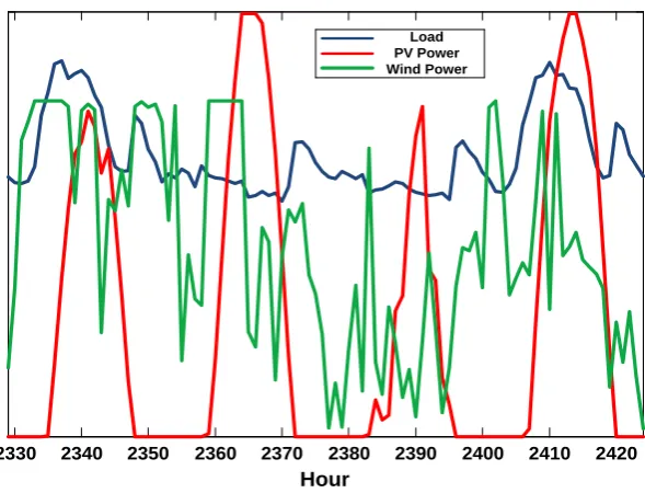
Figure 3.3. Generation of yearly curve shapes for distribution system analysis.

(22)

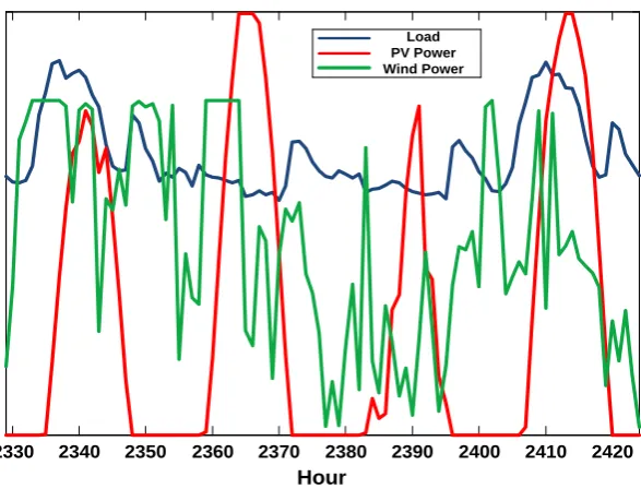
Figure 3.4. Curve shapes for node loads and renewable generation. 67

Figure 3.5. Diagram of the test system. 68

Figure 3.6. Impact of DG on the minimum voltage values. 69

Figure 3.7. Energy required from the HV system (measured at the secondary substation terminals).

69

Figure 3.8. Energy losses (without considering substation losses). 69

Figure 4.1. Block diagram of the implemented procedure. 78

Figure 4.2. Test system configuration and data. 79

Figure 4.3. Optimum location of one capacitor bank. Test system with 100 nodes; 1000 runs.

81

Figure 4.4. Optimum location of two capacitor bank with compensation ratio of 80%. Test system with 100 nodes; 1000 runs.

82

Figure 4.5. Optimum location of a single capacitor bank with a time varying load. Test system with 100 nodes; 1000 runs.

82

Figure 4.6. Profiles of load and generation (not with the same scale). 83

Figure 4.7. Optimum location of a single generation unit. Test system with 100 nodes; 1000 runs.

84

Figure 4.8. Optimum location of a single generation unit. Test system with 500 nodes; 5000 runs.

86

Figure 4.9. Optimum location of a single PV generation unit. Test system with 1000 nodes; 10000 runs.

88

Figure 4.10. Optimum location of a single wind generation unit. Test system with 1000 nodes; 10000 runs.

88

Figure 4.11. Profiles of load and generation. 91

Figure 4.12. Generation of random values for energy loss calculations – One generation unit.

93

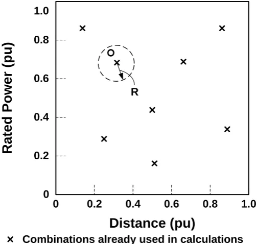
Figure 4.13. Pairing of n PV generation units in the Monte Carlo method to obtain the minimum distance between random values.

93

Figure 4.14. Pairing of PV generation units to obtain the distance between two Monte Carlo runs.

94

Figure 4.15. Test system configuration. 99

Figure 4.16. Configuration of a PV generator. 99

Figure 4.17. Load growth. 103

Figure 4.18. Sequential connection of optimum rated PV generators – Conventional Monte Carlo method.

106

Figure 4.19. Simulation results – Conventional Monte Carlo method – ZIP Model.

109

Figure 4.20. Power losses – First year. 111

Figure 5.1. Sequence of events after a failure. 121

(23)

Figure 5.3. Block diagram of the implemented procedure. 129

Figure 5.4. Test system configuration. 130

Figure 5.5. Time-current curves of protective devices. 132

Figure 5.6. Faulted element location. 135

Figure 5.7. Sequence of the system configurations after the occurrence of the fault.

136

Figure 5.8. Sequence of events after the occurrence of the fault. 137

Figure 5.9. Status of protective devices and switches after the occurrence of the fault.

137

Figure 5.10. Power measured at the substation terminals during protection system operation.

138

Figure 5.11. Power measured at the substation terminals during complete simulation.

139

Figure 5.12. Power injected by the PV generation units. 139

Figure 5.13. Power consumed from some affected load nodes. 140

Figure 5.14. Reliability indices – Probability density functions. 144

Figure 5.15. Location of failed element. 146

Figure 5.16. Failure of the voltage regulator located within the left-side feeder – Total load power.

148

Figure 5.17. Reliability indices – Probability density functions. 150

Figure A.1. OpenDSS structure [A.1]. 159

Figure A.2. OpenDSS element model [A.1]. 159

Figure A.3. Default solution loop [A.2]. 160

Figure A.4. OpenDSS user interface. 165

Figure A.5. Test system diagram. 168

Figure A.6. Master.dssfile. 169

Figure A.7. List.dss file. 170

Figure A.8. Circuit solution commands. 170

Figure A.9. Run script on user interface. 170

Figure A.10. Show and Plot examples. 170

Figure A.11. ShowLosses report file. 171

Figure A.12. ShowPowers report file. 171

Figure A.13. Output PlotCircuitPower. 172

Figure A.14. MATLAB - OpenDSS communication. 172

Figure A.15. DSSStartup function. 172

Figure A.16. Circuit solution command from MATLAB. 172

Figure A.17. Test system diagram. 175

(24)

Figure A.19. System information plots. 177

(25)

Chapter 1

1. Introduction

1.1. Problem Formulation

Currently it is widely accepted that the construction of large generation centers is no longer the best option to supply the increment of electric load. High costs related to the construction of new generation centers, state policies aimed at reducing the production of greenhouse gases, and legal issues, such as obtaining environmental permits for the construction of new transmission lines, are some of the main reasons that have driven the growth of small scale generation located close to actual load consumption, also known as Distributed Generation (DG). Distributed generation can also be encompassed within a much larger scope, the Distributed Energy Resources (DER) concept. DER refers to a variety of small, modular electricity-generating or storage technologies that can be aggregated to provide power necessary to meet regular demand and are installed at distribution level; distributed energy resources also includes demand-side management (i.e. energy efficiency and demand response) [1.1].

The introduction of distributed energy resources can provide great benefits for system operation. However, construction and connection of distributed generators cannot be made without considering the impact they will have on the system. Different planning studies must be carried out in order to ensure maximum benefits, normal operation, and foresee any eventual issues. The connection of distributed generation under non-optimal circumstances can have a negative impact on the system conditions and put normal operation at risk.

(26)

Analysis of Power Distribution Systems Using a Multicore Environment

2

In recent years many new methodologies have been developed to determine the optimum allocation of distributed generation [1.2]. Some of these methodologies rely on analytical approaches and assume many model simplifications [1.3]-[1.5], whereas others apply highly complex optimization algorithms [1.6]-[1.8]. The accuracy of these methods will depend on the solution approach and also the model used for representation of the distribution system.

Most current methods pursue the optimum allocation of distributed generators that constantly operate at rated capacity; therefore generation based on renewable resources (such as photovoltaic or wind generation) cannot be evaluated using these methodologies. Moreover, these methods fail to take into account the temporal nature of electric load (i.e. load behavior over time); consequently the optimum allocation of distributed generation is performed for one specific moment in time, rather than contemplating a larger evaluation period (e.g. one year). These are some of the aspects that need to be considered when developing new methods for the optimum allocation of distributed generation; furthermore, these new methodologies must be accurate, with a straightforward implementation, and time-efficient.

One aspect that can be improved with the introduction of distributed generation is the reliability of the distribution system. Distribution reliability is assessed through the estimation of system and load-point reliability indices [1.9]. Reliability indices can be calculated in a predictive or statistical manner; a predictive approach allows the validation of the reliability of a system design, whereas the statistical method can be used to monitor system performance over a determined period of time.

It is important for reliability methods to be able to cope with the possibility of system reconfiguration; that is, modifying the system topology in order to restore service to affected customers in the shortest time possible. The introduction of distribution generation further complicates the evaluation of reliability indices. Moreover, random nature of system failure causes reliability indices to show a varying behavior (i.e. they do not present constant values); therefore a proper analysis must be carried out in order to estimate this variation. The use of detailed system element models allows a more accurate calculation of reliability indices.

As a conclusion, it is clear that new methods for the evaluation of distribution reliability must be developed. These new methods must take into account the random nature of system failure, reconfiguration processes, the presence of distributed generation, and the response of system protection devices. Additionally, the new methods must be able to estimate the probability density function of reliability indices.

(27)

Chapter 1: Introduction

3

1.2. Power Distribution Systems

1.2.1. Power Systems General Structure

Power delivery systems are designed to collect electrical energy produced in large generation centers and transport it to the final load points where costumers demand it. Power delivery systems are comprised by other subsystems; in a deregulated market each subsystem is owned by a different company and free competition is permitted in each of them. The main subsystems in the power delivery system are presented in this sub-Section. Figure 1.1 shows the general structure of power systems [1.10]-[1.13].

Large Generation Centers

The great majority of electrical energy is produced using large generation units clustered in remote sites, far from final consumption points. Different technologies have traditionally been used to produce electrical energy in a large scale, such as nuclear, natural gas, coal, hydro, etc. Many of these plants were constructed in the past when the entire power system was owned by one company; lower costs and economies of scale allowed these companies to construct large yet still profitable plants.

Transmission System

The transmission system consists of a set of lines, substations, and equipment designed to connect large generation plants and consumption centers, power consumption is mainly carried out in cities and industrial areas. Lines belonging to the transmission system span over long distances and transport large quantities of energy; therefore, these lines operate at high-voltage levels (e.g. 400 and 220 kV).

Subtransmission System

The subtransmission system is an intermediary link between the transmission and the distribution system. The lines that compose the subtransmission system cover shorter distances than those in the transmission system; for that reason they operate at lower voltage levels (e.g. 132, 66, and 45 kV). An initial voltage reduction is required due to the difference in voltage level with respect to the transmission system. Large loads (such as big factories and other high consumption facilities) can be directly connected to the subtransmission system.

Primary Distribution System

(28)

4

the final customers. As in the subtransmission system, large loads can be connected to the primary distribution system.

Secondary Distribution System

The secondary distribution system consists of step-down (MV/LV) distribution transformers and low-voltage lines (e.g. 400 and 230 V) that deliver the energy to low power customers, such as commercial and residential loads.

Figure 1.1. Power delivery system structure [1.10].

1.2.2. Distribution System Structure

The distribution substation is the interconnection element between the distribution system and the upstream power delivery system. At the substation the step-down (HV/MV) transformer reduces the subtransmission voltage level to an appropriate value

Large generation centers

Transmission system

Subtransmission system

Primary distribution

system Secondary

(29)

5

for primary distribution lines. Different protection, switching, and measurement equipment is installed at the substation to ensure a safe operation. The primary distribution lines spread across the consumption area served by the substation, these primary distributions lines are also known as feeders. One or more lateral lines (or laterals) branch from distribution feeders and extend until they reach the step-down (MV/LV) distribution transformers, which are responsible for performing the final voltage reduction in order to obtain a voltage level adequate for customer use (e.g. 400 and 230 V). The secondary distribution lines operating at a low-voltage level transport the energy to the customer’s interconnection point; these lines are usually one-phase but there can also exist three-phase circuits. Overhead lines are primarily used in rural circuits, whereas in urban circuits distribution lines are mostly underground; in suburban areas there can be a mixture of overhead and underground circuits. Big industrial zones are usually served by dedicated circuits as they represent large loads that can affect the service of other loads. Figure 1.2 presents the typical configuration of a power distribution system, including the substation and the layout of one distribution feeder.

Figure 1.2. Typical distribution system configuration [1.10].

R

Circuit breaker or recloser Δ/Y

132/15 kV

Normally open

One-phase lateral circuit

Recloser

Three-phase lateral circuit Three-phase

(30)

6

1.2.3. Distribution System Primary Circuits

Primary distribution circuits are generally radial in design, unlike transmission systems where circuit designs are meshed. In comparison to meshed circuits, radial designs present certain advantages for power distribution: (1) protection is basically overcurrent, (2) lower fault currents, (3) voltage regulation and power flow control are easier to implement, and (4) system design is less expensive. The general radial circuit design can present different variations, such as the single feeder and open-loop configurations [1.11].

Single Feeder Configuration

Under this configuration all power demanded by laterals and secondary circuits is served by a single primary line; in case of failure or any other event that forces the feeder to be out of service (e.g. maintenance), all loads will experience a service interruption. The single feeder layout can also present a branched-configuration, where several branches stem from the original feeder in order to cover a larger area. These branches are not to be confused with laterals; laterals present a much lower current capacity, whereas the branches have the same (or similar) capacity as the main feeder. Figure 1.3 shows two examples of the single feeder configuration.

a) Simple feeder b) Branched-configuration

Figure 1.3. Single feeder configuration [1.11].

Open-loop Configuration

(31)

7

Figure 1.4. Open-loop configuration [1.11].

1.2.4. Distribution System Secondary Circuits

In rural and suburban areas a radial configuration is the most common design in secondary circuits; however, in urban circuits different configurations can be used depending on the type of load to be served. The spot configuration is used for large loads concentrated in one point (e.g. factories and large buildings), whereas the network configuration is used to serve a great number of loads distributed over a large area [1.11].

Radial Configuration

The radial design in distribution secondary circuits is equivalent to the configuration used in primary circuits. A secondary circuit parts from the step-down (MV/LV) distribution transformer and it spreads over the area where the customers are located; due to the size of the covered areas, the secondary circuits normally present a branched-configuration, see Figure 1.5a.

(32)

8

Spot Configuration

The spot configuration is used for loads that require dedicated circuits due to their high power demand; typically three or five feeders deliver the power demanded by the load, system design allows normal operation with the loss of one or two of the primary circuits. Each feeder arrives at a step-down (MV/LV) distribution transformer that serves part of the total load; all transformers are equipped with a protection device installed on its secondary side. A spot configuration is shown in Figure 1.5b.

a) Radial configuration b) Spot configuration [1.11]

Figure 1.5. Distribution secondary circuit configuration.

Network Configuration

In the network configuration several primary circuit lines feed the secondary network from multiple step-down (MV/LV) distribution transformers. The secondary circuits connected at the low-voltage side of the distribution transformers form a meshed network, from which the load power is provided. This configuration is used to serve commercial and residential loads (both three and one-phase). An example of a network configuration is presented in Figure 1.6.

1.2.5. Distribution System Substations

The configuration of a distribution substation will depend on the type of system served (urban, suburban, or rural); load level and desired reliability will affect the substation’s design and auxiliary equipment required [1.11].

Δ/Y o Y/Y 15/0.22 kV

Load Δ/Y o Y/Y

(33)

9

Figure 1.6. Network configuration [1.11].

Rural Substation

Substations designed for rural systems present a simple configuration; they consist of a single high-voltage and medium-voltage bus. Due to low load levels, a single transformer is enough to supply the entire power demand; transformer protection will depend on the transformer’s rated power. Primary distribution lines are connected to the medium-voltage bus and are protected by reclosers or overcurrent relays. Figure 1.7a presents the diagram of a rural substation.

Primary circuit

(34)

10

Suburban Substation

Suburban systems present higher load levels than rural systems; therefore more than one transformer will be necessary to serve the total system load. Suburban substations have a single bus on the high-voltage side, whereas each substation transformer has its own medium-voltage bus; medium-voltage buses are connected to each other through a normally-open tie-switch (see Figure 1.7b). In case of transformer failure, the tie-switch can be operated and the load corresponding to the failed transformer will be served by the remaining in-service transformers. This configuration known as split bus reduces fault levels, facilitates voltage control, and prevents the presence of circulating currents among transformers. Some utilities prefer to use a single medium-voltage bus for all substation transformers, which allows a more uniform load distribution among transformers.

a) Rural substation b) Suburban substation

Figure 1.7. Distribution substation configuration [1.11].

Urban Substation

The configurations in urban substations are more complex than those used for rural and suburban systems; two of the most common substation designs are the ring-bus and breaker-and-a-half configuration. In the ring-bus configuration, the medium-voltage buses form a closed loop with each section separated by a circuit breaker; distribution feeders and the secondary side of the substation transformers can be connected to the mid-point of any section, between two circuit breakers [1.14]. The breaker-and-a-half configuration consists of one or more branches connected between two medium-voltage buses, where each branch is made up of three circuit breakers. The secondary side of a substation transformer or primary distribution lines can be connected between any two adjacent circuit breakers [1.14]. Both configurations can be readily modified in order to carry out load transfer or perform maintenance on one of the circuit breakers. Figure 1.8 shows the diagram of two urban substations following the ring-bus and breaker-and-a-half configuration, respectively.

Δ/Y 132/15 kV

(35)

11

a) Ring-bus b) Breaker-and-a-half

Figure 1.8. Urban substation configuration.

1.2.6. Distribution System Elements

The safe operation of a power distribution system requires much dedicated equipment; this equipment is installed throughout the distribution system and it includes elements, such as power transformers, circuit breakers, and control and monitoring apparatuses. The most important elements and a brief definition are presented as follows.

Lines

Lines are responsible for transporting electrical energy between two distant points; overhead lines are typically made of bare aluminum (being ACSR a commonly used type), whereas underground lines commonly use cables with polymer-insulation, such as XLPE and EPR. Cables and conductors used for distribution lines are characterized by their current capacity and rated voltage [1.10].

Transformer

(36)

12

Circuit Breaker

A circuit breaker is a switching device designed to open and close a circuit by non-automatic means and to open the circuit non-automatically on a predetermined overcurrent in order to avoid damage to itself and other equipment [1.15].

Potential Transformer

A potential transformer is a conventional transformer with primary and secondary windings on a common core. Standard potential transformers are single-phase units designed and constructed so that the secondary voltage maintains a fixed relationship with primary voltage [1.15]. They are used to reduce the primary circuit voltage to a safe value (120 V), so it can be used as an input signal for monitoring and protection devices; these transformers only have the capacity to serve low rating meters and relays.

Current Transformer

A current transformer transforms line current into values suitable for standard protective and monitoring devices, and isolates the relays from line voltages. A current transformer has two windings, designated as primary and secondary, which are insulated from each other. The primary winding is connected in series with the circuit carrying the line current to be measured, and the secondary winding is connected to protective devices, instruments, meters, or control devices. The secondary winding supplies a current in direct proportion and at a fixed relationship to the primary current [1.15].

Relay

A relay is an electronic, low-powered device used to activate a high-powered device [1.16]. In distribution systems, relays protect feeders and system equipment from damage in the event of a fault by issuing tripping commands to the corresponding circuit breakers in order to interrupt the current produced by the fault.

Recloser

The automatic circuit recloser is a protective device with the necessary intelligence to sense overcurrents and interrupt fault currents, and to re-energize the line by reclosing automatically. In case of a permanent fault, the recloser locks open after a preset number of operations (usually three or four), isolating the faulted section from the main part of the system [1.17].

Fuse

(37)

13

and clearing times depend on the fuse’s time-current curves. The most commonly used fuses are the types K and T.

Sectionalizer

The sectionalizer is a circuit-opening device used in conjunction with source-side protective devices, such as reclosers or circuit breakers, to automatically isolate faulted sections of electrical distribution systems. The sectionalizer senses current flow above a preset level, and when the source-side protective device opens to de-energize the circuit, the sectionalizer counts the overcurrent interruption [1.17].

Switch

A switch is a switching device used to isolate a system element for repair or maintenance. It must be capable of carrying and breaking currents during normal operating conditions; a switch may include specified operating overload conditions and also carrying for a specified time currents under specified abnormal circuit conditions such as those of a short circuit. A switch, therefore, is not expected to break fault current, although it is normal for a switch to have a fault making capacity.

Voltage regulator

A voltage regulator is transformer with a 1:1 nominal transformation ratio equipped with an on-load tap changer; this device allows the transformer to vary its transformation ratio to react to voltage variations at the primary side. Voltage regulators are installed at intermediate points of long primary lines in order to compensate the voltage drop produced along the circuit; voltage control will impact the voltage profile of all loads downstream from the voltage regulator.

Capacitor Bank

A capacitor bank is a local source of reactive power. By correcting power factor it can perform voltage regulation and reduce system losses. Capacitor banks are generally three-phase and are installed within the distribution substation or at intermediate points of a primary circuit line.

SCADA

(38)

14

1.3. Distributed Generation

Distributed generation (DG) or embedded generation refers to generation applied at the distribution level [1.10]; DG units can be directly connected at the distribution substation or dispersed throughout the power distribution system. Due to their small size distributed generators can be placed close to load consumption, typically DG present sizes of up to 5 MW [1.10] (IEEE STD 1547 [1.19] applies for generators under 10 MW); however, utilities can limit the rated power of generation units according to their own operation policies [1.20].

The origins of distributed generation can be found in the “cogeneration” practiced by some industries; these generators serve a portion of the load at these industrial facilities and inject any excess of generation into the utility system; they also provide emergency power to the industrial facility during utility outages [1.21]. This is a common practice in industries such as pulp and paper, steel mills, and petrochemical facilities that had internal generation within their electrical facilities that operated in parallel with the utility system.

Costs reduction and efficiency improvement in small-size generators have turned distributed generation into an attractive option for utilities and independent producers. While the independent producer seeks to maximize its profits, utilities are concerned with exploiting the benefits of DG and improving system performance. The connection of distributed generation to the distribution system can be used for supporting voltage, reducing losses, providing backup power, providing ancillary services, or deferring distribution system upgrade [1.22]. Aspects to be considered when embedding DG into a distribution system are the great variety of generating technologies, or the intermittent nature of some renewable sources.

It is also important to remark the challenges and negative impacts that the connection of distributed generation can carry. Power distribution systems were not designed to host local generation; as a consequence of this design limitation, distributed generation can disrupt normal system operation. One of the most important concerns is the formation of undesired islands within the system [1.10]; under this condition an isolated section of the circuit is continued to be served by a local generator. Islanding (or island operation) can cause damage to distribution equipment and poses safety hazard for customers and utility personnel. In general, DG can cause miscoordination of protection devices and, if not properly handled, reduce reliability and power quality.

1.3.1. Distributed Generation Technologies

(39)

15

microturbines, fuel cells, Stirling engines, internal combustion engines, photovoltaic, and wind [1.23].

Microturbines

Microturbines are scaled down turbine engines with integrated generators and power electronics [1.23]. They operate at high speeds (about 100,000 rpm) and generate high-frequency AC power that is rectified by means of power electronics to comply with utility operating conditions. Microturbines can operate on a wide variety of gaseous and liquid fuels, and have extremely low emissions of nitrogen oxides. Electrical efficiency of microturbines is in the 25-30 percent range. Ancillary heat from microturbines can be used for water and space heating, process drying, food processing and absorption chilling.

Fuel Cells

A fuel cell is an electromechanical engine with no moving parts that collects the energy released from the combination of hydrogen and oxygen [1.23]. This reaction generates electricity, heat and water, while it produces almost no pollutants. In principle, a fuel cell operates like a battery; however, a fuel cell does not decay or require recharging; it will produce energy as long as fuel is supplied. The hydrogen needed for reaction in a fuel cell is typically produced from hydrogen rich fuels such as natural gas, propane, or methane from biogas recovery.

Stirling Engines

The Stirling engine is also known as an "external combustion engine”; it derives its power from heating and cooling a gas inside a sealed chamber with a piston. When the gas is heated, it will expand and build pressure within the sealed chamber; thus pushing a piston out [1.23]. When the gas cools, it will contract and pull the piston in. The Stirling engine runs cleaner and more efficiently than an internal combustion engine.

Internal Combustion Engines

The purpose of internal combustion engines is the production of mechanical power from the chemical energy contained in the fuel [1.24]. The expansion of hot gases produced during the combustion causes movement by acting on mechanical elements, such as pistons or rotors; the mechanical energy contained in this movement can be transferred to a generator, which transforms it into electrical energy. The most common internal combustion engine is the piston-type.

Photovoltaic

(40)

16

direct electric current. The key component of the BOS is the inverter; it is a power electronics device that converts the direct current generated by the solar cells into an alternating current. The Energy output of a PV generator depends on the amount of global radiation received and the generator’s technical specifications.

Wind

Modern wind energy systems consist of three basic components [1.23]: a tower (where the wind turbine is mounted), a rotor with blades, and the nacelle. The nacelle is a capsule-shaped component which contains auxiliary and electric equipment, including the generator. Wind turbines convert the wind’s kinetic energy transferred to their rotor into mechanical energy; a generator converts this mechanical energy into electricity. Actual power generation is mainly dependent on wind speed and the area covered by the turbine’s blades.

1.3.2. Distributed Generation and Loss Reduction

Distributed generation is operated according to its role in the system; two main modes of DG connection can be distinguished: (1) operating as a backup source within a microgrid; (2) operating in parallel with the distribution system.

Customers that require uninterrupted and highly reliable service may rely on internal generation to supply load demand in case of service interruption, i.e. they can operate as an island. This type of application can be found in critical loads (e.g. hospitals) and represents the operational core of a microgrid. Microgrids are defined as a small energy system capable of balancing captive supply and demand resources to maintain stable service within a defined boundary [1.26]; hence the presence of local generation is an essential element to the microgrid operation.

The operation of DG in parallel with the distribution system can contribute to relieve overburdened transmission and distribution facilities as well as reduce losses and voltage drop [1.10]. Distributed generation helps to reduce losses as it locally generates power demanded by loads, rather than producing it in large generation centers and forcing it to travel great distances to consumption points; the reduction achieved will depend on the generator’s rated power and location.

The optimum allocation of a generator injecting only active power in a radial feeder serving a uniformly distributed load is presented in [1.27]; according to this study, the maximum loss reduction is achieved by a generator of a rated capacity equal to 2/3 of the total load active power and located at 2/3 of the total feeder length (this is known as the 2/3 rule), this result is derived from the optimum allocation of capacitor banks presented in [1.10]. Although the 2/3 rule has limited practical application (system design is not realistic, and loads and DG are represented as constant current sources), the analysis carried out to obtain it can help to explain how DG helps to reduce system losses. Figure 1.9 presents the feeder current profile with and without DG; where I1 is

the total load current, Idg is the current injected by DG, and x is the distance from the

(41)

17

segment between the origin and DG location. A similar behavior can be found in other systems with a more complex design; however it will not be as easy to demonstrate the effect of DG, which is why this simple example is important to understand the way distributed generation influences system losses.

a) Without DG b) With DG

Figure 1.9. Feeder current profile.

1.4. Power Distribution Reliability

1.4.1. Introduction to Power Distribution Reliability

Reliability refers to a system’s ability to perform its required function under given conditions for a stated time interval [1.28]. From a power distribution system’s point of view, its function is to supply electrical energy to final customers without interruptions and within accepted tolerance margins (i.e. acceptable values for voltage and frequency) [1.29].

Power distribution systems are responsible for approximately 90% of all service interruptions experienced by customers [1.29]. Therefore, it is important to understand how the distribution system behaves and the effect that every element that composes it has in terms of system reliability; an accurate evaluation of power distribution reliability is essential to identify design weaknesses and areas within the system that require special attention.

A distribution system is composed by a great number of elements (see Section 1.2); a failure in one of these elements will affect the continuity of service provided to customers. The impact of element failure will depend on the element’s statistical parameters and system design [1.29]. The most important statistical parameters are the failure rate and the repair time. A failure rate is defined as the number of expected failures per element in a given time interval; while the repair time is the time required to restore service, whether by repairing or replacing the failed element [1.30]. The area affected by an element failure will depend on system design; a reliability-based design will include protection and switching devices, whose main task is to reduce the number of customers affected by a service interruption.

I1

0

I1

1pu x

I1

0 1pu

x

I1-Idg

(42)

18

The analysis of power distribution reliability is performed by following either a predictive or a statistical approach. These two approaches are not mutually exclusive as they both have different purposes and are carried out at different stages, but are equally relevant to the reliability evaluation of a power distribution system.

1.4.2. Predictive Analysis

Predictive analysis of power distribution system reliability can be used to validate system design as well as ensure that the reliability level provided meets utility policies and customer requirements. A great variety of methods have been developed for the predictive analysis of power distribution reliability, which can be classified into several categories; according to [1.31], these methods can be classified as: analytical and simulation-based methods.

Analytical methods

In analytical methods all system elements are represented by means of mathematical models. These methods use analytical equations in order to estimate system reliability indices; due to the complexity of real distribution systems, analytical methods generally rely on assumptions and simplification techniques. The evaluation of the analytical equations is rather straightforward and results can be found in a short period of time; however, developing the equations that model the system behavior can be a complex task, especially when considering reconfiguration processes and distributed generation.

The basic concepts of the analytical evaluation of power distribution systems are presented in [1.32]. The elements and segments that compose a distribution system are defined as follows:

1. General lateral section: it refers to lateral circuits branching from a feeder. It may include distribution transformers, line segments, and fuses.

2. General main section: it represents a main segment in a primary feeder or branch.

3. General series element: it is the series equivalent of any component, assumed for the purpose of easy calculation.

4. General feeder: a general feeder is a simple distribution system containing general main sections, general lateral sections and a general series component.

The following equations can be used to estimate the load point reliability indices when using the general feeder model.

Load point failure rate:

∑

= =

+ +

= m

k k k n

i i s

j p

1 1

λ λ

λ

(43)

19

Average outage duration:

∑

= =

+ +

= m

k

k k k n

i i i s

s

j r r p r

U

1 1

λ λ

λ ( 1.2 )

Average annual outage time:

j j j

U r

λ

= ( 1.3 )

where pk are the lateral section control parameters that depend on the fuse operation

mode; it can be 0, 1, and 2 corresponding to 100% reliable fuse, not fuse and a fuse operating not successfully with pk probability; λi, λk, and λs are the failure rate of the

main section, lateral section, and series element; ri, rk, and rs are the failure duration of

the three elements respectively. Failure duration times may vary depending on one of the following scenarios: (1) there is no alternate power supply; (2) the alternate power supply is 100% reliable; and (3) the alternate power supply is not 100% reliable, successful load transfer will depend on the availability probability pa.

Simulation-based methods

As the name implies, simulation-based methods rely on system simulation in order to analyze the reliability of the system under evaluation. The Monte Carlo method has been extensively used in power system reliability evaluation due to the random behavior presented by system failure [1.31]; this approach can be used in either sequential or non-sequential manner. In the application of the Monte Carlo method, random variables are generated to represent the state of system elements and times related to fault duration and service restoration. Simulation-based methods present a main disadvantage; that is, they require large computational efforts and long simulation times to obtain accurate results.

[1.31] presents a procedure for the evaluation of power distribution reliability based on a sequential Monte Carlo method; in this procedure each element is represented by a two-state model (Up and Down); the transition between these two states is defined by the parameters TTF and TTR. The time during which the element remains in the Up state is called the time to failure (TTF), whereas the time during which the element is in the down state is called the time to repair (TTR). Both TTF and TTR are random numbers defined by means of a probability density function (PDF).

In this procedure an artificial history that shows the Up and Down times of the system elements is generated in chronological order using random number generators and the probability distributions of the element failure and restoration parameters; see Figure 1.10.

(44)

20

Figure 1.10. Element Up/Down history [1.31].

Average failure rate:

∑

=

uj j j

T N

λ ( 1.4 )

Average outage time:

j dj j

N T

r =

∑

( 1.5 )

Average annual outage time:

∑

+ =

dj uj

dj j

T T

T

U ( 1.6 )

where j is the load point index, ∑Tu and ∑Td are the summations of all Up times (Tu)

and all Down times (Td) respectively, and Nj is the number of failures during the total

sampled years.

1.4.3. Statistical Analysis

Statistical analysis allows monitoring system performance from a reliability point of view; it also provides information that can help validate predictive analysis as well as identify areas where reliability needs to be improved. Statistical approaches require historical data of all service interruptions experienced by customers over a defined evaluation period. System reliability will be quantified by means of the customer interruption indices; the main indices are calculated according to the following equations [1.9].

System average interruption frequency index:

T n

i i

N N SAIFI

∑

=

= 1 ( 1.7 )

TTR TTF TTR

Up

Down

(45)

21

System average interruption duration index:

T n

i

i i

N H N SAIDI

∑

=

⋅

= 1 ( 1.8 )

Customer average interruption duration index:

SAIFI SAIDI

N H N

CAIDI _n

i i n

i

i i

= ⋅ =

∑

= =

1 1

( 1.9 )

Where k is the number of interruptions, Ni is the number of customer interrupted by a

fault, NT is the total number of customers in the system, and Hi is the duration of

interruption to customers interrupted by a fault.

The need of much detailed data for calculation of reliability indices may represent an important drawback for certain utilities as they do not possess the necessary facilities to keep record of every interruption experienced in their systems or lack an application that allows a prompt and easy access to it, posing an obstacle for an accurate evaluation of the system reliability.

1.5. Accomplishments

The work in this Thesis has been oriented at developing a procedure for the optimum allocation of distributed generation and another procedure for reliability evaluation of distributed systems; both procedures are based on the Monte Carlo method.

The procedure for optimum allocation of distributed generation has been developed to determine the quasi-optimum rated power and location of one or more generation units when the objective is to achieve the maximum energy loss reduction; it is capable of evaluating any system regardless of its topology or model used for load representation. Energy system losses are calculated by simulating the system for the specified evaluation period; the procedure can cope with different evaluation periods, ranging from one year to up to 10 years or more. The general Monte Carlo procedure was refined in order to reduce the number of necessary executions; the new methods introduced as “Refined Monte Carlo” and “Divide and Conquer” were tested and proved to cause a reduction in total simulation times without loss in the results accuracy.

(46)

22

Due to their Monte Carlo nature both developed methods are time consuming and require a large number of runs/samples to obtain accurate results. As a result it was necessary to introduce new techniques in order to reduce total simulation times; parallel computing was the tool chosen to achieve this goal. Thanks to the application of parallel computing it was possible to execute both methods in affordable times without any loss in accuracy. Additionally, these methods require information regarding the load and generation behavior over the evaluation period; therefore, three algorithms were implemented in order to obtain node load profiles, and solar and wind generation curves. These three algorithms allow the user to generate the necessary information without having to rely on external tools (e.g. HOMER [1.33]).

As a result of the research work carried out for this Thesis, several technical papers have been submitted to different conferences and journals. The complete list of accepted and submitted papers is as follows:

1. J.A. Martinez and G. Guerra, “Optimum placement of distributed generation in three-phase distribution systems with time varying load using a Monte Carlo approach,” IEEE PES General Meeting, San Diego, July 2012.

2. J.A. Martinez and G. Guerra, “A Monte Carlo approach for distribution reliability assessment considering time varying loads and system reconfiguration,” IEEE PES General Meeting, Vancouver, July 2013.

3. J.A. Martinez and G. Guerra, “A Parallel Monte Carlo method for optimum allocation of distributed generation,” IEEE Trans. on Power Systems, vol. 29, no. 6, pp. 2926-2933, November 2014.

4. G. Guerra and J.A. Martinez, “A Monte Carlo method for optimum placement of photovoltaic generation using a multicore computing environment,” IEEE PES

General Meeting, National Harbor, USA, July 2014.

5. J.A. Martinez and G. Guerra, “A Parallel Monte Carlo approach for distribution reliability assessment”, IET Gener., Transm. Distrib., vol. 8, no. 11, pp. 1810-1819, November 2014.

6. J.A. Martinez-Velasco and G. Guerra, “Analysis of large distribution networks with distributed energy resources”, Ingeniare, vol. 23, no. 4, pp. 594-608, October 2015.

7. G. Guerra, J.A. Corea-Araujo, J.A. Martinez, and F. Gonzalez-Molina, “Generation of bifurcation diagrams for ferroresonance characterization using parallel computing,” EEUG Conf., Grenoble (France), September 2015.

8. G. Guerra and J.A. Martinez, “Optimum allocation of distributed generation in multi-feeder systems using long term evaluation and assuming voltage-dependent loads,” Sustainable Energy, Grids and Networks, vol. 5, pp. 13-26, March 2016.

9. J.A. Martinez and G. Guerra, “Reliability Assessment of Distribution Systems with Distributed Generation Using a Power Flow Simulator and a Parallel Monte Carlo Approach,” Submitted for publication in Sustainable Energy, Grids and

Networks.

10.J.A. Martinez-Velasco and G. Guerra, “Allocation of Distributed Generation for Maximum Reduction of Energy Losses in Distribution Systems,” Chapter 12 of

Energy Management of Distributed Generation Systems, InTech, In editing

(47)

23

1.6. Document Structure

The remainder of this Thesis is divided into five subsequent Chapters and one Appendix. The Chapters will present the procedures developed for the Thesis as well as detail case studies used to prove the usefulness of the proposed methods. The following Chapters are organized as follows.

Second Chapter

The Second Chapter makes a brief introduction of the main concepts of parallel computing. It also introduces the “Multicore for MATLAB” library, which is the tool chosen for individually accessing system cores and implementing multicore computing. Finally, it presents how the “Multicore for MATLAB” library can be used in conjunction with OpenDSS for the application of parallel computing to the simulation of power distribution systems.

Third Chapter

The Third Chapter presents the three algorithms implemented for the generation of node load profiles, and PV and wind generation curves. A short example is presented to demonstrate the information that can be generated with these three algorithms and how it can be used in different studies.

Fourth Chapter

The Fourth Chapter presents the developed procedure for the optimum allocation of distributed generation, including how this procedure was implemented to be executed in a multicore environment. Furthermore, two refinements of the proposed Monte Carlo approach aimed at reducing total execution times are presented. The implemented procedure is tested in different systems and the main results and conclusions are presented in this Chapter.

Fifth Chapter

Analysis of power distribution systems using a multicore environment

PhD Thesis

Analysis of Power Distribution Systems

Using a Multicore Environment

Luis Gerardo Guerra Sánchez

Analysis of Power Distribution Systems

Using a Multicore Environment

Luis Gerardo Guerra Sánchez

Dissertation submitted to the Doctorate Office

of the Universitat Politècnica de Catalunya in

partial fulfillment of the requirements for the

degree of Doctor of Philosophy by the

UNIVERSIDAD DE MALAGA

UNIVERSIDAD DE SEVILLA

UNIVERSIDAD DEL PAÍS VASCO/EUSKAL ERRIKO UNIBERTSITATEA

UNIVERSITAT POLITÈCNICA DE CATALUNYA

Joint Doctoral Programme in

Electric Energy Systems

Acknowledgments

List of Publications

Journal Publications:

Conference Publications:

Book Chapters:

Table of Contents

List of Tables

List of Figures

Chapter 1

1.

Introduction

1.1.

Problem Formulation

1.2.

Power Distribution Systems

1.2.1.

Power Systems General Structure

1.2.2.

Distribution System Structure

1.2.3.

Distribution System Primary Circuits

1.2.4.

Distribution System Secondary Circuits

1.2.5.

Distribution System Substations

1.2.6.

Distribution System Elements

1.3.

Distributed Generation

1.3.1.

Distributed Generation Technologies

1.3.2.

Distributed Generation and Loss Reduction

1.4.

Power Distribution Reliability

1.4.1.

Introduction to Power Distribution Reliability

1.4.2.

Predictive Analysis

∑

∑

∑

∑

∑

∑

∑

∑

∑

1.4.3.

Statistical Analysis

∑

∑

∑

∑

1.5.

Accomplishments

1.6.

Document Structure