Essays in structural macroeconometrics

(1)

Essays in Structural Macroeconometrics

Fernando José Pérez Forero

TESI DOCTORAL UPF / ANY 2013

DIRECTOR DE LA TESI

(2)

(3)

List of Figures

1.1 Posterior estimates of . . . 8 1.2 Acceptance rates of the single-move algorithm . . . 28 1.3 Median and posterior 68 percent tunnel, volatility of monetary

policy shock. . . 30 1.4 Estimates of . . . 31 1.5 Dynamics following a monetary policy shock, different dates. . . . 32 1.6 Long-run effects of monetary policy shocks . . . 32 1.7 Time varying and time invariant responses. . . 33 2.1 Posterior distribution of the Monetary Policy Stance, median value

and 90 percent posterior bands . . . 50 2.2 Monetary Policy Stance and NBER recession dates (shaded areas) 51 2.3 Historical Decomposition of Monetary Policy index and NBER

recession dates (shaded areas) . . . 53 2.4 Weights of various instruments in the Monetary Policy index,

me-dian value and 90 percent con dence bands . . . 54 2.5 Responses to Monetary Policy shocks in 1996, 90 percent con

d-ence interval . . . 56 2.6 Responses to Monetary Policy shocks in 2012, 90 percent con

d-ence interval . . . 57 2.7 Response of the Federal Funds Rate to an expansionary NBR

policy shock . . . 57 2.8 Policy rule coef cients, median value and 90 percent bands . . . . 59 2.9 Standard Deviation of Policy shock s

t . . . 60

2.10 Sensitivity to Demand shocks d

t . . . 63

2.11 Sensitivity to Discount window shocks b

t . . . 63

2.12 Comparison of Standard Deviation of Policy shock s

t . . . 64

(8)

3.4 Model implied dispersion i;t . . . 87

3.5 Responses ofstandXtto" f t,"bt and t . . . 88

A.1 Inef ciency factor for each parameter of the model . . . 103

A.2 Plot of 6;t . . . 103

A.3 Plot of 9;t . . . 104

A.4 Rolling Covariance Matrix of MCMC draws . . . 105

A.5 Histograms for 11;t, selected dates. . . 105

A.8 Volatility of monetary policy shock (single-move) . . . 107

A.9 Impulse responses to monetary shocks (single-move) . . . 108

A.10 Estimates for (single-move) . . . 108

B.1 Responses after a Monetary Policy shocks and before the Great Financial Crisis, 90 percent bands . . . 110

B.2 Responses after a Monetary Policy shocks after the Great Finan-cial Crisis, 90 percent bands . . . 110

B.3 Inef ciency Factor IF for each parameter in the model . . . 120

B.4 MCMC draws of parameter 6;t . . . 120

B.5 MCMC draws of parameter d t . . . 121

B.6 Cumulative variances of vector t . . . 122

B.7 Cumulative variances of vector_ect . . . 122

B.8 Histograms of parameter d t . . . 123

C.1 ER and Interest differentials . . . 126

C.2 Details about Predicted Exchange Rates by Industries data, BoJ . . 127

C.3 Reference to Predicted Exchange Rates (TANKAN), FAQ of The Bank of Japan . . . 127

C.4 Convergence in mean . . . 128

(9)

List of Tables

1.1 Identi cation restrictions . . . 24

1.2 Acceptance Rates from multi-move routine . . . 28

2.1 Priors . . . 48

3.1 Posterior estimates for 2000-2012 . . . 84

(10)

(11)

(12)

(13)

Acknowledgements

In rst place, I would like to thank Fabio Canova and Kristoffer Nimark for their continuous support and guidance during the development of this thesis. I also thank them for giving me the opportunity to undertake different research projects as co-author and therefore allowing me to gain experience as a researcher.

I also would like to thank Vasco Carvalho, Jordi Galí, Christian Matthes, Bar-bara Rossi and all the faculty members and PhD Students of Pompeu Fabra who actively participate in the CREI Macroeconomics Breakfast. Their very valuable comments and suggestions at every stage of my research gave me the possibility of completing it.

In addition, I would like to thank Marta Araque and Laura Agustí for be-ing there every time I needed help with many administrative procedures at UPF. Thanks also to Mariona Novoa for her help in scheduling my presentations. Thanks to them for their invaluable ef ciency.

During these years I have made a lot of friends. I thank to all of them for the opportunity to share tons of experiences. Thanks to Miguel and Mapi for all the moments we spent together, starting from the problem sets in 2008 until being atmates in the last year 2012-2013. Thanks to the `Peruvian Community', starting with Miguel (again), Cynthia, Sofía and Silvio. Thanks to Marc and Jorg for having the opportunity to share our opinions about research, football, history and religion. I would like to also mention the people with whom I had great times during these years: Rodrigo, Benjamín, Mauro, Giorgio and Paula, Mapi (again) and Davide, Oriol, Sergio and Johanna, Elisa, José, Alicia, José, José Carlos, Jagdish, Tom and Michael. Please forgive me if I forgot anyone. Thanks to my of ce mates Ciccio, Tanya, Vicky and Bruno. Thanks to the musicians Ciccio (again), Kiz, Miguel Karlo and Gene for giving me the opportunity to play the guitar with them, you rock!

(14)

(15)

Abstract

This thesis is concerned with the structural estimation of macroeconomic mod-els via Bayesian methods and the economic implications derived from its empir-ical output. The rst chapter provides a general method for estimating structural VAR models. The second chapter applies the method previously developed and provides a measure of the monetary stance of the Federal Reserve for the last forty years. It uses a pool of instruments and taking into account recent practices named Unconventional Monetary Policies. Then it is shown how the monetary transmis-sion mechanism has changed over time, focusing the attention in the period after the Great Recession. The third chapter develops a model of exchange rate de-termination with dispersed information and regime switches. It has the purpose of tting the observed disagreement in survey data of Japan. The model does a good job in terms of tting the observed data.

Resumen

(16)

(17)

Foreword

This thesis is concerned with the structural estimation of macroeconomic mod-els via Bayesian methods and the economic implications derived from its out-put. It is mainly developed within the context of structural vector autoregressive (SVAR) models and general state space models.

The rst chapter,” A general algorithm for estimating structural VARs”, is a joint work with the professor Fabio Canova. It provides the method for estimating structural VAR models, which are non-recursive and potentially overidenti ed, with both constant and time varying coef cients. The procedure allows for linear and non-linear restrictions on the parameters, maintains the multi-move structure of standard algorithms and can be used to estimate structural models with different identi cation restrictions. The transmission of monetary policy shocks is studied with the proposed approach and results are compared with those obtained with traditional methods.

The second chapter, “Measuring the Stance of Monetary Policy in a Time-Varying world”, applies the method previously developed and focuses its attention in measuring the monetary policy stance. The stance of monetary policy is of gen-eral interest for macroeconomists and the private sector. But it is not necessarily observable, since a Central Bank can use different instruments at different points in time. This chapter provides a measure of this stance for the last forty years using a pool of instruments. Different operating procedures are quanti ed by comput-ing the time varycomput-ing weights of these instruments and takcomput-ing into account recent practices named Unconventional Monetary Policies. The measure describes how tight/loose was monetary policy conduction over time and takes into account the uncertainty related with posterior estimates of the parameters. Then it is shown how the monetary transmission mechanism has changed over time, focusing the attention in the period after the Great Recession.

(18)

(19)

Chapter 1 A GENERAL ALGORITHM FOR

ESTIMATING STRUCTURAL

VARS (JOINT WITH F. CANOVA)

1.1 Introduction

1

Vector autoregressive (VAR) models are routinely employed to summarize the properties of the data and new approaches to the identi cation of structural shocks have been suggested in the last 10 years (see Canova and De Nicoló (2002), Uhlig (2005), and Lanne and Lütkepohl (2008)). Constant coef cient structural VAR models may provide misleading information when the structure is changing over time. Cogley and Sargent (2005) and Primiceri (2005) were among the rsts to estimate time varying coef cient (TVC) VAR models and Primiceri also provides a structural interpretation of the dynamics using recursive restrictions on the mat-rix of impact responses. Following Canova et al. (2008), the literature nowadays mainly employes sign restrictions to identify structural shocks in TVC-VARs and the constraints used are, generally, theory based and robust to variations in the parameters of the DGP, see Canova and Paustian (2011).

While sign restrictions offer a simple and intuitive way to impose theoret-ical constraints on the data, they are weak and identify a region of the parameter space. Furthermore, several implementation details are left to the researcher mak-ing comparison exercises dif cult to perform. Because of these features, some investigators still prefer to use ”hard” non-recursive restrictions, using the termin-ology of Waggoner and Zha (1999), even though these constraints are not

theoret-1_{We would like to thank F. Schorfheide, G. Primiceri, R. Casarin, H. Van Dijk and three}

(20)

ically abundant. Algorithms to estimate non-recursive structural models exist, see e.g. Waggoner and Zha (2003) or Kociecki and Ca' Zorzi (2013). However, their extension to overidenti ed or TVC models is problematic.

This paper proposes a general framework to estimate a structural VAR (SVAR) that can handle time varying coef cient or time invariant models, identi ed with hard recursive or non-recursive restrictions. The procedure can be used in sys-tems which are just-identi ed or overidenti ed, and allows for both linear and non-linear restrictions on the parameter space. Non-recursive structures have been extensively used to accommodate models which are more complex than those per-mitted by recursive schemes. As shown, e. g., by Gordon and Leeper (1994), in-ference may crucially depend on whether a recursive or a non-recursive scheme is used. In addition, although just-identi ed systems are easier to construct and es-timate, over-identi ed models have a long history in the literature (see e.g. Leeper et al. (1996), or Sims and Zha (1998)), and provide a natural framework to test interesting hypotheses.

TVC-VAR models are typically estimated using a Bayesian Gibbs sampling routine. In this routine, a state space system is speci ed, the parameter vector is partitioned into blocks, and draws for the posterior are obtained cycling through these blocks. When stochastic volatility is allowed for, an extended state space representation is used and one or more parameter blocks are added to the routine. If a recursive contemporaneous structure is assumed, one can sample the block of contemporaneous coef cients equation by equation, taking as predetermined draws for the parameters belonging to previous equations. However, when the sys-tem is non-recursive, such an approach disregards the restrictions existing across equations. Hence, the sampling must be done differently.

To perform standard calculations, one also needs to assume that the covariance matrix of the contemporaneous parameters is block-diagonal. When the structural model is overidenti ed, such an assumption may be implausible. However, relax-ing the diagonality assumption complicates the computations since the blocks of the conditional distributions used in the Gibbs sampling do not necessarily have a known format. Primiceri (2005) suggests to use a Metropolis-step to deal with this problem. We follow his lead and nest the step into Geweke and Tanizaki (2001)'s approach to estimate general nonlinear state space models. This setup is conveni-ent since it can accommodate general non-linear idconveni-enti cation restrictions. Thus, many structural systems can be dealt with in a compact and uni ed way.

(21)

time variations translate in important changes in the transmission of monetary policy shocks which are consistent with the idea that the ability of monetary policy to in uence the real economy has waned, especially in the 2000s. We also show that the characterization of the dynamics in response to monetary policy shocks one obtains in an overidenti ed but xed coef cient VAR is different.

The paper is organized as follows, Section 2 builds up intuition, shows how to apply the algorithm to estimate a simple SVAR with time invariant coef cients, and the identi cation restrictions that are allowed for. Section 3 extends the setup to a time varying coef cients static SVAR. Section 4 presents the general algorithm that is applicable to non-recursive, overidenti ed TVC-VAR models with stochastic volatility and quite general identi cation restrictions. Section 5 studies the transmission of monetary policy shocks. Section 6 summarizes the conclusions.

1.2 Constant coef cients static SVAR

To build the intuition, we start from a static SVAR with constant coef cients A( )yt ="t; "t N(0; IM) (1.1)

wheret= 1; : : : ; T;ytand"tareM 1vectors,A( )is a non-singularM M

matrix and a vector of structural parameters. The likelihood function of (1.1) is

L yT _j = (2 ) M T =2det (A( ))T exp

(

1 2

T

X

t=1

(A( )yt)0(A( )yt)

)

(22)

1.2.1 Reparameterization of the SVAR

There are a number of ways to reparametrize the SVAR. Here we show that they are equivalent in terms of the likelihood.

Amisano and Giannini's setup

In Amisano and Giannini (1997), the matrixA( )is re-parametrized as vec(A( )) =SA +sA

Since

(A( )yt)0(A( )yt) = tr (A( )yt)0(A( )yt)

tr (A( )yt)0(A( )yt] = [vec(A( )yt)]0[vec(A( )yt)]

vec(A( )yt) = (yt0 IM) (SA +sA) (1.3)

after a number of manipulation (see on-line appendix), the likelihood for the re-parametrized model can be written as

L yT _j = (2 ) M T =2det (A( ))T exp

(

1 2

T

X

t=1

(3 0S_A0 +s_A0 ) (IM yt0yt)

(SA + 2sA)

)

(1.4)

Waggoner and Zha's setup

Waggoner and Zha (2003) rewrite theA( )matrix as A( ) = a1 a2 aM

= _U1 1+R1 U2 2+R2 UM M +RM

such that = 0₁ 0₂ 0_M 0 is the original column vector. That is, they perform a linear transformation of each of the columns ofA( ). This reparamet-erization allows them to develop a sampling routine where each i,i= 1; : : : ; M

is drawn from a mixture of normal and gamma distributions. For the sake of concreteness, suppose that:

A( ) =

2 4

1 0 3

1 1 0

0 2 1

3

(23)

so that the system is non-recursive and overidenti ed (we require that the vari-ances of the shocks are unity). The Amisano and Giannini's reparameterization is

vec(A( )) =

2 6 6 6 6 6 6 6 6 6 6 6 6 4 1 1 0 0 1 2 3 0 1 3 7 7 7 7 7 7 7 7 7 7 7 7 5 = 2 6 6 6 6 6 6 6 6 6 6 6 6 4

0 0 0 1 0 0 0 0 0 0 0 0 0 0 0 0 1 0 0 0 1 0 0 0 0 0 0

3 7 7 7 7 7 7 7 7 7 7 7 7 5

| {z }

SA

2 4 12

3

3 5

| {z }

+ 2 6 6 6 6 6 6 6 6 6 6 6 6 4 1 0 0 0 1 0 0 0 1 3 7 7 7 7 7 7 7 7 7 7 7 7 5

| {z }

sA

The Waggoner and Zha reparameterization is

a1 =

2 4 1 1 0 3

5; _U1 =

2 4 0 1 0 3

5; _R1 =

2 4 1 0 0 3

5; 1 = 1

a2 =

2 4 0 1 2 3

5; _U2 =

2 4 0 0 1 3

5; _R2 =

2 4 0 1 0 3

5; 2 = 2

a3 =

2 4 03

1

3

5; _U3 =

2 4 1 0 0 3

5; _R3 =

2 4 0 0 1 3

5; 3 = 3

Clearly

vec(A( )) =

2 4 a1 a2 a3 3 5 so that

SA=diag(U1;U2;U3) ; sA =

2 4 R_R12

R3

3 5

wherediag(:)indicates a block-diagonal matrix. Hence, Waggoner and Zha re-parameterization also delivers the likelihood(1:4).

Alternative re-parametrization

Vectorizing(1:1)produces

(24)

Using(1:3)and the fact thatvec("t) = "t, the model can be expressed as:

e

yt=Zt +"t (1.6)

where y_et (yt0 IM)sA; Zt (yt0 IM)SA. The likelihood function of

(1.6) is (see Appendix A.1 for details)

e

L yT _j = (2 ) M T =2(detD)T exp

(

1 2

T

X

t=1

[_eyt Zt ]0[eyt Zt ]

)

(1.7)

whereD= @[vec(A( )yt)]

@y0

t =Dy+Dz,vec(Dy) = sAandvec(Dz) = SA . Thus

vec(D) = vec(A( ))

and the likelihood in (1.7) is equal to the likelihood in (1:4). Note that (1.6) tells us that estimates of can be obtained using data correlations. For the example in equation (1.5), (1.6) is equivalent to the following three linear regressions:

y1t = y2t 1+ 1t

y2t = y3t 2+ 2t

y3t = y1t 3+ 3t (1.8)

1.2.2 The proposal distribution and the MH algorithm

The advantage of the reparameterization in (1.6) is that it allows us to easily design a proposal distribution to be used in a Metropolis routine. First, get estimates of the parameters in (1.6)

=

" _T X

t=1

Z_t0Zt

# 1" _T

X

t=1

Z_t0_eyt

#

(1.9)

and of the covariance matrix

P ( ) =

" _T X

t=1

Z_t0(SSE) 1Zt

# 1

(1.10)

whereSSE = PT_t₌₁(_eyt Zt ) (yet Zt )0. Then, the algorithm to draw is

as follows. Set 0 = and fori= 1;2; : : : ; G:

1. Draw a candidate _y p ( i j i 1) = t( i 1; rP ( i 1); ), where

(25)

2. Compute = pe( yjyT)p ( i 1j i)

e

p( i 1jyT)p ( ij i 1), wherep(:e jy

T_{) =}_L(ye T

j:)p(:)is the pos-terior kernel of( _y; i 1). Draw av U(0;1). Set i = yifv < !and

i = i 1 otherwise, where

! minf ;1g; ifI ( y) = 1 0; ifI ( _y) = 0

HereI (:)is a truncation indicator andGis the total numbers of draws. Note that sinceP (:), depends on , the algorithm can be easily nested into a Gibbs sampling scheme. A t-distribution with small number of degrees of freedom is chosen to account for possible deviations from normality: when is large the proposal resembles a normal distribution.

Notice two facts about this algorithm. First, the vector is jointly sampled. Second, the covariance matrix of P ( ) is generally non-diagonal. As we ex-plain later, these features distinguish our algorithm from those in the literature and provides the exibility needed to accommodate a variety of structural models. Kociecki and Ca' Zorzi (2013) have derived a closed form solution for the posterior of under the assumption thatdet(A) = 1. Interestingly, their posterior collapses to our proposal when the prior for is diffuse.

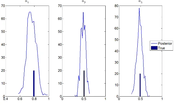
1.2.3 A Numerical example

We illustrate the properties of our Metropolis approximation in the example of equation (1.5), when = 0:8 0:5 0:5 0. We simulate data according to (1:1)fort = 1; : : : ;500, re-parametrize the model as in(1:6)and estimate and P using(1:9)and(1:10). We use at priors, i.e.,p( i)/ 1; i= 1;2;3. We set

G= 150;000, discard the rst100;000, and keep1every100from the remaining. The acceptance rate is24%.

Figure 1.1 indicates that the simulator does a good job in reproducing the DGP (the vertical lines indicate true values).

1.2.4 Identi cation restrictions

(26)

[image:26.595.157.437.131.300.2]

Figure 1.1: Posterior estimates of

Short-run linear restrictions

Suppose

A( ) =

2 4

1 0 2

1 1 0

0 2 1

3 5

vec(A( )) =

2 6 6 6 6 6 6 6 6 6 6 6 6 4 1 1 0 0 1 2 2 0 1 3 7 7 7 7 7 7 7 7 7 7 7 7 5 = 2 6 6 6 6 6 6 6 6 6 6 6 6 4 0 0 1 0 0 0 0 0 0 0 0 1 0 1 0 0 0 0 3 7 7 7 7 7 7 7 7 7 7 7 7 5

| {z }

SA

1 2

| {z }

+ 2 6 6 6 6 6 6 6 6 6 6 6 6 4 1 0 0 0 1 0 0 0 1 3 7 7 7 7 7 7 7 7 7 7 7 7 5

| {z }

sA

Since the restrictions are linear, the setup ts the above framework.

Short-run non-linear restrictions

Suppose now

A( ) =

2 4

1 0 3

1 1 0

0 ( 2+ 1)2 1

3

(27)

The model is re-parametrized as

vec(A( )) =

2 6 6 6 6 6 6 6 6 6 6 6 6 4 1 1 0 0 1 ( 2+ 1)2

3 0 1 3 7 7 7 7 7 7 7 7 7 7 7 7 5 = 2 6 6 6 6 6 6 6 6 6 6 6 6 4

0 0 0 1 0 0 0 0 0 0 0 0 0 0 0 0 1 0 0 0 1 0 0 0 0 0 0

3 7 7 7 7 7 7 7 7 7 7 7 7 5

| {z }

SA

2

4 ( 2+ 1)1 2 3

3 5

| {z }

F( )

+ 2 6 6 6 6 6 6 6 6 6 6 6 6 4 1 0 0 0 1 0 0 0 1 3 7 7 7 7 7 7 7 7 7 7 7 7 5

| {z }

sA

where F ( ) is a non-linear vector-valued function. Linearity is lost here, but if we de ne _e2 ( 2+ 1)2 as a new parameter, the procedure applies to the

vector _e = ( 1;e2; 3). In fact, given posterior draws for e2, we can recover 2 =

p

e2 1once we impose the extra restrictione2 >0. Adding this restriction

avoids us to deal with the fact thatF( )is non-linear. Consider now:

A( ) =

2 4

1 0 3

1 1 0

0 ( 2+ 2 3)2 1

3

5 (1.12)

Here

F ( ) =

2

4 ( 2+ 21 3)2 3

3 5

Also in this case the procedure can be employed, if we de ne_e2 ( 2+ 2 3) 2

as a new parameter. In fact, with draws from the posterior of_e2 and 3, we can

recover 2 =

p

e2 2 3, provided thate2 >0.

Consider a nal example:

A( ) =

2 4

1 0 1 2 1

1 1 0

0 2 1

3

(28)

The reparametrized model is

vec(A( )) =

2 6 6 6 6 6 6 6 6 6 6 6 6 4 1 1 0 0 1 2 1 2 1

0 1 3 7 7 7 7 7 7 7 7 7 7 7 7 5 = 2 6 6 6 6 6 6 6 6 6 6 6 6 4

0 0 0 1 0 0 0 0 0 0 0 0 0 0 0 0 1 0 0 0 1 0 0 0 0 0 0

3 7 7 7 7 7 7 7 7 7 7 7 7 5

| {z }

SA

2

4 12

1 2 1

3 5

| {z }

F( )

+ 2 6 6 6 6 6 6 6 6 6 6 6 6 4 1 0 0 0 1 0 0 0 1 3 7 7 7 7 7 7 7 7 7 7 7 7 5

| {z }

sA

where = [ 1; 2]0. Here linearity is lost and adding an inequality constraint does

not help since the third component of F( ) depends on the other two. Letting zt( ) ZtF ( ), the model is:

e

yt=zt( ) +"t

In general, if a closed-form solution for combinations of the parameters is available, the procedure can deal with short run non-linear restrictions. However, when a closed-form is not available, we need to treat the model as a non-linear system of equations, and the tools we describe in section 4 are useful.

Long-run restrictions

Long run restrictions are non-linear, but can be dealt in our Metropolis algorithm with a accept/reject step. To see this consider the more general SVAR model:

A( )yt=A+yt 1 +"t; "t N(0; IM) (1.14)

LettingB [A( )] 1A+, the VAR is:

yt =Byt 1 + [A( )] 1"t (1.15)

The (long run) cumulative matrix is:

D (IM B) 1[A( )] 1 (1.16)

Given draws ofBand ;one can immediately constructDusing (1.16) and check whether the required restrictions are satis ed. For example, suppose the cumulat-ive impact matrix is restricted as

D =

2 4

D11 D12 0

0 D22 D23

D13 0 D33

(29)

This set of restrictions can be summarized as

R0vec(D) =

2 4

0 0 0

3

5 (1.17)

with

R0 =

2 4

0 1 0 0 0 0 0 0 0 0 0 0 0 0 1 0 0 0 0 0 0 0 0 0 1 0 0

3 5

From(1:15)settingy_bt yt Byt 1, we have that

A( )_byt ="t

where

A( ) =

2 4

1 3 5

1 1 6 2 4 1

3

5 (1.18)

To estimate the structural parameters, we need rst to drawB, then draw candidate 's using the suggested reparameterization and for each draw use an accept-reject step to make sure the long run restrictions(1:17)are satis ed. Seen through these lenses, long run and non-linear short run restrictions are similar. Clearly, if par-tial multipliers or the structural lagged coef cients A+ are restricted with zero

constraints, the same acceptance/rejection framework can be used.

A situation that leads to a non-linear model is one where there are both long and short run restrictions (see e.g. Gali (1991)). For example, suppose

D =

2 4

D11 D12 D13

0 D22 D23

D31 D32 D33

3 5

and in (1.18) 4 = 5 = 0. Let

(IM B) 1

2

4 bb1121 bb1222 bb1323

b31 b32 b33

3 5

Then

D = 1 detA( )

2 4

b11 b12 b13

b21 b22 b23

b31 b32 b33

3 5

2 4

1 4 6 4 5 3 3 6 5

2 6 1 1 2 5 1 5 6 1 4 2 2 3 4 1 1 3

(30)

Thus,D21= 0implies b21( 4 6 1) b23( 2 1 4) b22( 1 2 6) = 0

and, using 4 = 0and 5 = 0, we have b22( 1 2 6) = 0. Hence, long run

restrictions require 1 = 2 6and the impact matrix is

A( ) =

2 4

1 3 0

2 6 1 6 2 0 1

3 5

Therefore

vec(A( )) =

2 6 6 6 6 6 6 6 6 6 6 6 6 4 1 2 6 2 3 1 0 0 6 1 3 7 7 7 7 7 7 7 7 7 7 7 7 5 = 2 6 6 6 6 6 6 6 6 6 6 6 6 4

0 0 0 0 1 0 0 0 0 1 0 0 0 0 1 0 0 0 0 0 0 0 0 0 0 0 0 0 0 0 0 1 0 0 0 0

3 7 7 7 7 7 7 7 7 7 7 7 7 5

| {z }

SA 2 6 6 4 2 6 2 3 6 3 7 7 5

| {z }

F( )

+ 2 6 6 6 6 6 6 6 6 6 6 6 6 4 1 0 0 0 1 0 0 0 1 3 7 7 7 7 7 7 7 7 7 7 7 7 5

| {z }

sA

Sign restrictions

Although sign restrictions are not the focus of this paper, it is straightforward to show that the algorithm can be applied also to VARs identi ed this way. LetA( ) be a general matrix with no zero elements and impose inequality constraints on, say, the rst column. Then, one can draw 's as in section 2.2 and check if the rst column satis es the required inequality restrictions. Thus, sign restrictions can be dealt with in the same way as long run restrictions.

1.3 Time-varying coef cients static SVAR

Before we move to a full edged TVC-SVAR model, it is useful to study the intermediate step of a static TVC-SVAR. The model is

A( t)yt="t; "t N(0; IM) (1.19) t= t 1+ t; t N(0; V) (1.20)

whereV is positive de nite and 0is given. This model is re-parametrized as:

e

(31)

t= t 1+ t (1.22)

where, as before,_eyt (yt0 IM)sAandZt (yt0 IM)SA. We wish to

com-putep T

jyT_{; V} _and_{p V}

jyT_; T _{to be used in the Gibbs sampler. Given the}

assumptions the latter is inverted Wishart and its parameters are easy to compute. Using the Markovian structure of the model, the conditional posteriorp T

jyT_{; V}

can be factorized as

p T _jyT; V = p( T jyT; V) T_Y1

t=1

p t j t+1; yt; V

/ p( T jyT; V) T_Y1

t=1

p t jyt; V p( t+1 j t; V)(1.23)

Since each term in the last expression is normal, to sample T _{from (1.23) we just}

need the mean and the variance of each of the terms.

Thus, set initial values 0 andP0j0 and for eacht= 1; : : : ; T construct

btjt 1 = bt 1jt 1

Ptjt 1 =Pt 1jt 1+V

and the Kalman gainKt =Ptjt 1Zt0

1

t , where t =Zt0Ptjt 1Zt+IM:Estimates

of tand of its variance are updated according to

btjt = btjt 1+Kt yet Ztbtjt 1

Ptjt = Ptjt 1 Ptjt 1Zt0

1

t ZtPt0jt 1

To smooth the estimates set _T_j_T =_bTjT,P_T_j_T =PTjT and, fort=T 1; : : : ;1;,

compute

tjt+1 =btjt+PtjtZt0P

1

t+1jt t+1jt+2 Zt0btjt

P_t_j_t₊₁ =Ptjt PtjtZt0P

1

t+1jtZtPt0jt 1

1.3.1 The basic algorithm

Step 1: Given yT; Vi 1 ;we take an initial value T0 =f 0;tg T t=1and:

1. Computen (i 1)

tjt+1

oT

t=1 and

n

P_t_j(_t₊₁i 1)oT

t=1.

2. At eacht = 1; : : : ; T, draw a candidate _y_t p ( tj i 1;t) =t i 1;t; rP

(i 1)

tjt+1 ; ,

r >0, 4. Setp T _j T_i ₁ =

T

Y

t=1

(32)

3. Compute = p(( y)

T₎_p ₍ T i 1j

T₎

p( T

i 1)p ( Tj Ti 1)

wherep(:)is the posterior kernel(1:23). Draw a v U(0;1). Set T_i = ( _y)T if v < ! and set T_i = T_i ₁ otherwise, where

! minf ;1g; ifI ( y)

T _{= 1}

0; ifI ( _y)T _{= 0}

andI (:)is a truncation indicator function. Step 2: Given( T

i ; yt), drawVi from(Vi 1 j Ti ; yt) W vV; V

1

, where vV =T +vV

V 1 =

"

V +

T

X

t=1

( t t 1) ( t t 1)0

# 1

wherev_V andV are prior parameters. We then use T

i ; Vi as initial values and repeat steps1and2fori= 1; : : : ; G.

Given the structure of the problem, if is constant,V is the null matrix. Thus, Kalman smoother and OLS estimates andP will coincide and the algorithm collapses to the one described in section 2.2.

1.4 A time-varying coef cients SVAR

Assume that aM 1vector of non-stationary variablesyt; t = 1; : : : ; T can be

represented with a nite order autoregression of the form:

yt=B0;tCt+B1;tyt 1+:::+Bp;tyt p+ut (1.24)

whereB0;t is a matrix of coef cients on aM 1vector of deterministic variables

Ct;Bj;t;j = 1; : : : ; pare square matrices containing the coef cients on the lags

of the endogenous variables andut N(0; t), where tis symmetric, positive

de nite, and full rank for everyt. For the sake of presentation, exogenous vari-ables are excluded, but the setup can be easily extended to account for them. Since (1:24)is a reduced form,utdoes not have an economic interpretation. Denote the

structural shocks by"t N(0; IM)and let

ut=At1 t"t (1.25)

whereAt A( t)is the contemporaneous coef cients matrix and t=diagf i;tg

(33)

whereX0

t=IM Ct0; y0t 1; : : : ; yt p0 andBt = vec(B0;t)0; vec(B1;t)0; : : : ; vec(Bp;t)0 0

are aM K matrix and aK 1vector, K = M M +pM2_{. It is typical to}

assume that(Bt; At; t)evolve as independent random-walks:

Bt = Bt 1+ t (1.27)

t = t 1+ t (1.28)

log ( t) = log ( t 1) + t (1.29)

where tdenotes the vector of free parameters ofAt, and let:

V =V ar

0 B B @ 2 6 6 4

"t t t t

3 7 7 5

1 C C

A=

2 6 6 4

I 0 0 0

0 Q 0 0

0 0 V 0

0 0 0 W

3 7 7

5 (1.30)

where Q; V; W are full rank matrices. Common patterns of time variations are possible if the rank of some of these matrices is reduced.

Thus, the setup captures time variations in i) the lag structure (see (1:27)), ii) the contemporaneous reaction parameters (see (1:28)) and iii) the structural variances (see(1:29)):As shown in Canova et al. (2012), models with breaks at a speci c date can be accommodated by adding restrictions on the law of motions (1:27) (1:29).

1.4.1 Relaxing standard assumptions

Consider the concentrated model obtained with estimates of the reduced-form coef cientsBbt:

At yt Xt0Bbt Atbyt = t"t (1.31)

As before, let

vec(At) =SA t+sA (1.32)

whereSAandsAare matrices with ones and zeros of dimensions M2 dim( )

and M2 _1;_{respectively. The concentrated model can be reparametrized as}

(_by_t0 IM) (SA t+sA) = t"t

and the state space is composed of

e

yt=Zt t+ t"t (1.33)

of (1.28) and (1.29), where _eyt (yb0t IM)sA; Zt (yb0t IM)SA; . Given

(34)

The standard approach is to partition tinto blocks associated with each

equa-tion, say t = 1t0; 2t0; : : : ; Mt 0

0

;and assume that these blocks are independent, so thatV =diag(V1; : : : ; VM). Under these assumptions

p T _j_eyT; T;_V;BcT ₌ M

Y

m=2

p m;T _j m 1;T;_eyT; T;_V;BcT (1.34)

p 1;T _jy_eT; T;_V;BcT

Thus, for each equationm, the coef cients in equationm j; j 1are treated as predetermined and changes in coef cients across equations are uncorrelated. The setup is convenient because equation by equation estimation is possible. Since the factorization does not necessarily have an economic interpretation, it may make sense to assume that the innovations in the tblocks are uncorrelated. However, if

we insist that each element of thas some economic meaning, the diagonality of

V is no longer plausible. For example, if tcontains policy and non-policy

para-meters, it will be hard to assume that non-policy parameters are strictly invariant to changes in the policy parameters (see e.g. Lakdawala (2011)).

The algorithm to draw we have described relaxes both assumptions, that is, the vector tis jointly drawn andV is not necessarily block diagonal. This

modi-cation allows us to deal with recursive, non-recursive, just-identi ed or overiden-ti ed structural models in a uni ed framework.

In a constant coef cient SVAR one identi es shocks imposing short run, long run, or heteroschedasticity restrictions. In TVC-VARs identi cation restrictions are typically employed only on At but, as we have seen, certain type of

restric-tions produce non-linear state space models. In some situarestric-tions one may want to identify shocks imposing shape restrictions on certain medium term multipliers (the maximum effect of a monetary shock on output occurs x-months after the disturbances) or on the variance decomposition, as it is done in the news shock literature (see e.g. Barsky and Sims (2012)), and these may also generate non-linear structural VARs. Furthermore, while it is standard to employ a log non-linear setup for the time variations inlog( t), one may want to use GARCH or Markov

switching speci cations, which also generate a non-linear or non-normal law of motion for some of the coef cients.

To be able to deal with all these cases, we embed the Metropolis algorithm to draw T _{into a modi ed version of Geweke and Tanizaki (2001)'s routine for}

(35)

1.4.2 Estimation

Consider the general state space model:

b

yt = zt( t) +ut( t; 1t) (1.35) t = tt( t 1) +rt( t 1; 2t) (1.36)

ht( t) = kt( t 1) + 3t (1.37)

wherey_bt, 1t; 3tareM 1vectors; tand 2tareK 1vectors; 1t N(0; Q1t),

2t N(0; Q2t), 3t N(0; Q3t). Assume thatzt(:),tt(:),rt(:); ut(:); ht(:); kt(:)

are vector-valued functions.

To estimate this system, it is typical to linearize it around the previous forecast of the state vector, so that

zt( t) ' zt(batjt 1) +Zbt( t batjt 1)

ut( t; 1t) ' ut(btjt 1;0) +bu ;t( t btjt 1) +bu 1;t 1;t

tt( t 1) ' tt(bat 1jt 1) +Tbt( t 1 bat 1jt 1)

rt( t 1; 2t) ' rt(bt 1jt 1;0) +rb;t( t 1 bat 1jt 1) +br2;t 2;t

ht( t) ' ht(btjt 1) +bht( t btjt 1)

kt( t) ' kt(btjt 1) +bkt( t btjt 1)

whereZbt,bu ;t,ub1;t,Tbt,rb;t,rb2;t,bht;bktare matrices corresponding to the Jacobian

ofzt(:),ut(:),tt(:),rt(:),ht(:); kt(:), evaluated at t=batjt 1; t =btjt 1, 1;t =

0, ₂_;t= 0. Thus, the approximated model is

b

yt ' Zbt t+dbt+bu 1;t 1;t (1.38)

t ' Tbt t 1+cbt+br 2;t 2;t (1.39) b

ht t ' bkt t 1+fbt+ 3t (1.40)

where

b

dt=zt batjt 1 Zbtbatjt 1+u(btjt 1;0) bu ;t(btjt 1 t) (1.41)

b

ct =tt bat 1jt 1 Tbtbat 1jt 1+rt(btjt 1;0) br ;t(btjt 1 at 1) (1.42)

b

ft=kt btjt 1 bktbtjt 1 ht btjt 1 +bhtbtjt 1 (1.43)

Equations(1:38);(1:39);(1:40)are similar to equations(1:33)and(1:28),(1:29). Whenzt(:); tt(:);

kt(:); ht(:); ut(:)are linear, rt is independent of t andut is independent of t. dbt = 0, cbt = 0,fbt =0. In one of the cases considered by Rubio Ramírez et

al. (2010) or in some of those of section 2.4dbt 6=0, while if the law of motion of

(36)

The algorithm

Set initial values for (BT

0; T0; T0; sT0;V0), where sT is J-dimensional vector of

discrete indicator variables described below. Then: 1. DrawBT

i from fromp BiT j Ti 1; Ti 1; siT 1;Vi 1 IB BiT ;whereIB(:)

truncates the posterior to insure stationarity of impulse responses. 2. Draw T

i from

p T_i _jy_b_iT; _iT ₁; sT_i ₁;_Vi 1 / p i;T jybTi ; i 1;T; si 1;T;Vi 1

T_Y1

t=1

p i;t jbyit; i 1;t; si 1;t;Vi

pt+1( i;t+1 j i;t; i 1;t; si 1;t;Vi 1)

using the Metropolis approach described in section 3.1, where ijt+1; Pijt+1

are estimated with the extended Kalman smoother (EKS) described below. 3. Draw T

i using a log-normal approximation as in Kim et al. (1998). Given

B_iT; T_i , the model is linear and composed of

b

Ateyt =yt = t"t

and (1:29), but the error is not normal. The m th equation is y_m;t =

m;t"m;t, where m;tis them th diagonal element of t. Then

y_t = logh y_m;t 2+ci 2 log ( m;t) + log"2m;t (1.44)

where c is a small constant. Since "m;t is Gaussian, log"2m;t is log ( 2)

distributed. Such a distribution can be approximated by a mixture of nor-mals. Conditional onst, the indicator for the mixture of normals, the model

is linear and Gaussian. Hence, standard Kalman smoother recursions can be used to draw_f tgT_t₌₁ from(1:44) (1:29). To ensure independence of

the structural variances, each element of_f m;tgM_m₌₁ is sampled assuming a

diagonalW. 4. To drawsT

i , given( Ti ,yt), drawu U(0;1)and compare it to

P sm;t =j jym;t;log ( m;t) /qj

y_m;t 2 log ( m;t) j+ 1:2704 j

wherej = 1; : : : ; J; (:)is the normal density function,qj a set of weights,

the term inside the parenthesis is the standardized error termlog"2

(37)

j and j are the mean and the standard deviation of thej th mixture

com-ponent. Then assignsm;t =j iffP sm;t j 1jym;t;log ( m;t) < u

P sm;t j jym;t;log ( m;t) .

5. Draw_Vi fromp Vi j Ti ;byiT; Ti 1; sTi 1 . The matrixVi is sampled

assum-ing that each block follows an independent inverted Wishart distribution. Then one usesBT_i ; T_i; T_i ; sT_i ;_Vias initial values and repeat the sampling for

the ve blocks fori= 1; : : : ; G. The details of step 2

Given (yT_; T_{), we predict the mean and mean square error of}

tfort= 1; : : : ; T:

batjt 1 =tt(bat 1jt 1)

Ptjt 1 =TbtPt 1jt 1Tbt0+br2;tQ2tbr 0

2;t

and compute the Kalman gain Kt = Ptjt 1Zbt0

1

t , where t = Zbt0Ptjt 1Zbt +

b

u ₁;tQ2tbu0₁;t.

As new information arrives, estimates are updated according to

b

atjt =batjt 1+Kt yt zt batjt 1

Ptjt=Ptjt 1 Ptjt 1Zbt0

1

t ZbtPt0jt 1

To smooth the estimates, set _T_j_T =_baTjT,P_T_j_T =PTjT and compute

tjt+1 =batjt+PtjtZbt0P

1

t+1jt t+1jt+2 tt(batjt)

P_t_j_t₊₁ =Ptjt PtjtZbt0

h

Pt+1jt+br 2;tQ2tbr 0

2;t i 1

b

ZtPt0jt 1

for t = T 1; : : : ;1;. To start the iterations, we use_ba1j0 = 0K 1 and P0j0 =

IK ; >>1. Notice that the approximate model is used only in predicting and

updating the mean square error of .

1.4.3 Discussion

(38)

variables, and rare (and large) shocks hit the economy. The alternative would be to use recently developed sequential Montecarlo methods, see e.g., Creel (2012) and Herbst and Schorfheide (2013), to compute the posterior of the unknown of the non-linear state space model. While such an approach is feasible, it complic-ates computations quite a lot. As it will be clear in the application section, our approach allows us to estimate medium scale VARs in reasonable amount of time. Furthermore, in most applications identi cation restrictions imply a linear state space. Thus, it is important to have a tool that can extensively cover that situation and can deal with certain non-linear restrictions used in the literature without hav-ing to pay the full costs of havhav-ing a complete non-linear methodology.

1.4.4 Single-move Metropolis for drawing

B

t

To draw BT _{in step 1 of the algorithm one can employ a standard multi-move}

strategy where the components ofBT _{are jointly sampled from normal}

distribu-tions having moments centered at Kalman smoother estimates. Koop and Potter (2011) have argued that multi-move algorithms are inef cient when one requires stationarity of the impulse responses at each t; especially if the VAR is of me-dium/large dimension. The assumption of non-explosive impulse responses is appealing in many macroeconomic applications and since Cogley and Sargent (2005), it is common to assume that all the eigenvalues of the companion form matrix associated withBtlie within the unit circle fort = 1; : : : ; T. Thus, draws

that do not satisfy the restrictions are discarded. When the Carter and Kohn (1994) a multi-move logic is used, if one element of the sequences violates the restric-tions, the entire sequence is discarded, making the algorithm inef cient.

To solve this problem, Koop and Potter suggest to evaluate the elements of the BT _{sequence separately using a single-move algorithm and use an accept/reject}

step. The approach works as follows. Given draws ofBT

i 1; Ti 1; Ti 1; Qi 1; Vi 1; Wi 1,

the measurement equation is

yt=Xt0Bt+At1 t"t

and the transition equation forBtis

Bt =Bt 1+ t

with t N(0; Q); B0 given, andAt1 t"t = ut N(0; t). To sample the

individual elements ofBT_{, all}_t _1:

1. Draw a candidateBc

t N( t; t)where t =

( _B

t 1;i+Bt+1;i 1

2 +Gt

h

yt Xt0

Bt 1;i+Bt+1;i 1

2

i

(39)

Gt=

1

2Qi 1Xt(Xt0Qi 1Xt+ t)

1

; t < T Qi 1Xt(Xt0Qi 1Xt+ t)

1

; t=T

t=

1

2 (IK GtXt0)Qi 1 ; t < T

(IK GtXt0)Qi 1 ; t=T

2. Construct the companion form matrixBc_tand evaluate1 max eig Bc_t <1 , where 1(:) is an indicator function taking the value of 1 if the condition within the parenthesis is satis ed.

3. The acceptance rate ofBc t is

!B;t = min

8 < :

1(maxjeig(Bct)j<1)

(Bc t;Qi 1)

1 (Bt;i 1;Qi 1)

;1 9 = ; = min (

1 max eig Bc_t <1 (Bt;i 1; Qi 1)

(Bc

t; Qi 1)

;1

)

where (:) is an integrating constant, measuring the proportion of draws that satisfy the inequality constraint. To compute (:)one rst drawsB_tc;l N(B_tc; Qi 1), for l = 1; : : : ; L, constructs the companion form matrix

Bc;l_t and evaluates l = 1 max eig B c;l

t <1 . Second, one evaluates

(Bc

t; Qi 1) =

XL

l=1

l

L and (Bt;i 1; Qi 1)and compute the acceptance

probability. Whent=T, this probability is !B;T =1 max eig B

c t <1

4. Draw a v U(0;1). Set Bt;i = Btc if v < !B;t and set Bt;i = Bt;i 1

otherwise.

SinceQdepends on Bt, we need to change the sampling scheme also for this

matrix. Assume a-priori thatQ 1 _{W v; Q} 1 _{so that the unrestricted posterior}

isQ 1 _{W v; Q} 1 _with_v ₌_v₊_T _and

Q 1 =

"

Q+

T

X

t=1

(Bt;i Bt 1;i) (Bt;i Bt 1;i)0

# 1

To draw Q we need to draw a candidate (Qc₎ 1

W v; Q 1 and take the inverse Qc_{. Then, for} _t _{= 1; : : : ; T}_{, we evaluate} _(B

(40)

for a xedL;and calculate the acceptance probability

!Q = min

( _T

Y

t=1

(Bt;i; Qi 1)

(Bt;i; Qc)

;1

)

Finally, we draw av U(0;1), setQi =Qc ifv < !QandQi =Qi 1otherwise.

In a standard multi-move approach (:) = 1, when sampling bothBT andQ. Therefore, Koop and Potter's approach generalizes the multi-move procedure at the cost of making convergence to the posterior, in general, much slower, and, as we will see later on, of adding considerable computational time.

1.4.5 A shrinkage approach

To deal with the stationarity issue one could also consider the shrinkage approach of Canova and Ciccarelli (2009). The approach was originally designed to deal with the curse of dimensionality in large scale panel VAR models, but can also be used in our context. The main problem with the standard setup is that when Bt is of large dimension and each of the components is an independent random

walk, the probability that explosive draws for at least one coef cient are obtained is very large at each t. By makingBt function of a lower dimensional vector of

factors t, who independently move as a random walk, the approach can reduce

the computational costs and the inef ciency of the algorithm.

The model is still consists of (1.26), (1.28) and (1.29) but now (1.27) is sub-stituted by

Bt = t+ t t N(0; I) (1.45)

t = t 1+ t t N(0; Q) (1.46)

wheredim( t) dim(Bt)and where the matrix is known and composed of

ones and zeros as in Canova and Ciccarelli (2009). The setup where the matrix is unknown and estimated along the other unknown quantities is presented in the on-line appendix. Using (1.46) into (1.45) we have

yt =Xt0 t+At1 t"t+Xt0 t Xt0 t+ t (1.47)

where t N(0M 1; Ht)withHt At1 t 0t A

1

t

0

+X0

tXt.

To estimate the unknowns we do the following:

1. Sample T _{using a multi-move routine using (1.47) and (1.46).}

2. Given T_{, we compute}

b

yt =yt Xt0 t. Pre-multiplying byAt, we get the

concentrated structural model

(41)

As before

(_by_t0 IM) (SA t+sA) = t"t+AtXt0 t

so that the second state-space system is

e

yt = Zt t+ t"t+AtXt0 t (1.48)

t = t 1+ t (1.49)

and we draw T _{using our proposed Metropolis step. Here, the variance}

of the measurement error is t 0t+At( t)Xt0XtA0t( t)and it is evaluated

at the current prediction tjt 1. T is sampled using the extended Kalman

smoother previously described. 3. Given( T, T_):

b

Atybt= t"t+AbtXt0 t

SinceAbtXt0is known, let the lower-triangularPtsatisfyPt AbtXt0XtAb0t Pt0 =

I. Then

PtAbtbyt =yt =Pt t"t+PtAbtXt0 t

with var PtAbtXt0 t = I and where Pt t 0tPt0 +Pt AbtXt0XtAb0t Pt0 is

a diagonal matrix. This transformation is similar to Cogley and Sargent (2005); however, since AbtXt0 is known, we only need to sample the

vari-ances of m;t. As in algorithm 4.2.1, we do this using thelog( 2)

approx-imation that consists on a mixture of 7 normals (see (1.44)).

4. Given( T; T_; T_{), we sample}_{Q; V; W} _{from independent inverted Wishart}

distributions as in algorithm 4.2.1.

5. Given new values of m;t, we construct At1 t 0t A

1

t

0

+X_t0Xt and go

back to step 1.

We evaluate the relative merits of different approaches in the speci c example discussed in the next section.

1.5 An Application

(42)

1.5.1 The SVAR

The vector of endogenous variables isyt= (GDPt; Pt; Ut; Rt; Mt; P comt)0, where

GDPtis a measure of aggregate output,Pta measure of aggregate prices,Ut the

unemployment rate, Rt the nominal interest rate, Mt a monetary aggregate and

P comtrepresents a commodity price index. Since researchers working with this

set of variables are typically interested in the dynamic response to monetary policy shocks, see e.g. Sims and Zha (2006), the structure ofAtis restricted as in table

1, whereXindicates a non-zero coef cient.

Reduced form_nStructuralGDPtPtUtRtMtP comt

Non-policy 1 1 0 0 0 0 0

Non-policy 2 X 1 0 0 0 0

Non-policy 3 X X 1 0 0 0

Monetary policy 0 0 0 1 X 0

Money demand X X 0 X 1 0

[image:42.595.196.442.261.371.2]

Information X X X X X 1

Table 1.1: Identi cation restrictions

The structural form is identi ed via exclusion restrictions as follows:

1. Information equation: Commodity prices(P comt)convey information about

recent developments in the economy. Therefore, they react contemporan-eously to all structural shocks.

2. Money demand equation:Within the period money balances;are a function of structural shocks to core macroeconomic variables(Rt; GDPt; Pt).

3. Monetary policy equation: The interest rate(Rt)is used as an instrument for

controlling the money supply(Mt). No other variable contemporaneously

affects this equation.

4. Non-policy block: Following Bernanke and Blinder (1992), the non-policy variables (GDPt; Pt; Ut) react to policy, money or informational changes

only with a delay. This setup can be formalized by assuming that the private sector uses only lagged values of these variables as states or that private decisions have to be taken before the current values of these variables are known. The relationship between the variables in the non-policy block is left unmodeled and, for simplicity, a recursive structure is assumed.

(43)

are likely to be correlated. Let"t = "1t "2t "3t " mp

t "mdt "it

0 _{be the vector}

of structural innovations. The structural model is

2 6 6 6 6 6 6 4

1 0 0 0 0 0

1;t 1 0 0 0 0

2;t 5;t 1 0 0 0

0 0 0 1 11;t 0

3;t 6;t 0 9;t 1 0

4;t 7;t 8 10;t 12;t 1

3 7 7 7 7 7 7 5

| {z }

At 2 6 6 6 6 6 6 4 GDPt Pt Ut Rt Mt

P comt

3 7 7 7 7 7 7 5

=A+_t (L)

2 6 6 6 6 6 6 4

GDPt 1

Pt 1

Ut 1

Rt 1

Mt 1

P comt 1

3 7 7 7 7 7 7 5 + t 2 6 6 6 6 6 6 4

"1_t "2

t

"3

t

"mp_t "md t "i t 3 7 7 7 7 7 7 5 (1.50) whereA+_t (L)is a function ofAtandBtand we normalize the main diagonal ofAt

so that the left-hand side of each equation corresponds to the dependent variable. Finally, t= 2 6 6 6 6 6 6 4 1

t 0 0 0 0 0

0 2

t 0 0 0 0

0 0 3_t 0 0 0

0 0 0 mp_t 0 0

0 0 0 0 md

t 0

0 0 0 0 0 i_t

3 7 7 7 7 7 7 5

is the matrix of standard deviations of the structural shocks.

The structural model (1:50) is non-recursive and overidenti ed by 3 restric-tions. Overidenti cation obtains because the policy equation is different from the Taylor rule generally employed in the literature. It is easy to check (see on-line appendix) that the (constant coef cient version of the) system is globally identi-ed and therefore suitable for interesting policy experiments. While the structural model we consider is conditionally linear, more general non-linear models are easy to generate using the restrictions described in section 2.4 or considering a non-linear law of motion for the parameters. Our setup can accommodate for all these possibilities.

1.5.2 The Data

The data we use comes from theInternational Financial Statistics (IFS)database at the International Monetary Fund and from the Federal Reserve Board (www. imfstatistics.org/imf/about.asp and www.federalreserve.gov/econresdata/

(44)

Domestic Product index (Volume, base 2005=100), the commodity prices index, and M2 are from IFS, the Federal Funds rate is from the Fed. All the variables are expressed in year-to-year rate changes, i.e. y_t = log (yt) log (yt 4), except

for the Federal Funds and the unemployment rate, and standardized, that is,xt =

(y_t E(y_t))=std(y_t), to have all the variables on the same scale.

1.5.3 The prior and computation details

The VAR is estimated with 2 lags; this is what the BIC criteria selects for the con-stant coef cient version of the model. The priors are proper, conjugate for

compu-tational convenience and given byB0 N B;4 VB ,Qprior IW k2Q VB;(1 +K) ,

0 N( ; diag(abs( ))), Sprior IW(kS2 diag(abs( ));(1 + dim )),

log ( 0) N( ;10 IM),W prior

i IW(k

2

W;1 + 1); i= 1; : : : ; M.

To calibrate the parameters of the prior, we use the rst 40observations as a training sample:BandVBare estimated with OLS and and with Maximum Likelihood using100different starting points with the constant coef cient version of the model. We setk2

Q = 0:5 10 4,kS2 = 1 10 3; kW2 = 1 10 4andJ = 7.

We generate150;000 draws, discard the rst100;000 and use one every100 of the remaining for inference. Convergence was checked using standard statistics -see on-line appendix. Draws forBt are monitored and discarded if the stability

condition fails. The indicator functionI (:); used to eliminate outlier draws, is uniform over the interval( 20;20):In our application all draws were inside the bounds. The acceptance rate for the Metropolis step is35:6percent.

Since the structural model hasM = 6, anddim( ) = 12, then

sA= [e01; e02; e30; e04; e05; e06]

0

whereei are vectors inRM with

ei = [ei;j] M

j=1 such thatei;j =

(45)

and also

SA=

2 6 6 6 6 6 6 6 6 6 6 6 6 6 6 6 6 6 6 6 6 6 6 6 6 6 6 6 6 6 6 6 6 6 6 6 6 4

01 dim( )

1 01 (dim( ) 1)

01 (2 1) 1 01 (dim( ) 2)

01 dim( )

01 (3 1) 1 01 (dim( ) 3)

01 (4 1) 1 01 (dim( ) 4)

02 dim( )

01 (5 1) 1 01 (dim( ) 5)

01 dim( )

01 (6 1) 1 01 (dim( ) 6)

01 (7 1) 1 01 (dim( ) 7)

05 dim( )

01 (8 1) 1 01 (dim( ) 8)

04 dim( )

01 (9 1) 1 01 (dim( ) 9)

01 (10 1) 1 01 (dim( ) 10)

03 dim( )

01 (11 1) 1 01 (dim( ) 11)

01 dim( )

01 (12 1) 1 01 (dim( ) 12)

06 dim( )

3 7 7 7 7 7 7 7 7 7 7 7 7 7 7 7 7 7 7 7 7 7 7 7 7 7 7 7 7 7 7 7 7 7 7 7 7 5

Finally, computations were performed on an Intel (R) CORE(TM) i5-2400 CPU @ 3.1GHz machine with 16GB of RAM.

1.5.4 Multi-move, single move, shrinkage algorithms

The Carter and Kohn (1994) routine is fairly popular in the literature. However, when one needs to impose stationarity of the impulse responses, it becomes very inef cient, in particular in situations like ours, when the SVAR has more than three variables and year-on-year growth rates of the variables are used. The problem can be somewhat diminished if quarterly growth rates are used, since they tend to be less persistent2 _{and considerably reduced if data is standardized. We show these}

facts in table 1.2, which reports the acceptance rates in the four possible options.

In the Koop and Potter's algorithm, we setL = 25;when evaluate the integ-rating constants (:) in each period. The priors, the number of draws and the skipping scheme are the same as in the multi-move algorithm. The averages ac-ceptance rates for BT are 97% and 91% for year-on-year and quarterly growth

(46)

Detrending_nScales Non-standardized Standardized Year-on-year growth rates 0:46% 10:2%

Quarterly growth rates 0:60% 11:5% Table 1.2: Acceptance Rates from multi-move routine

Year-on-year, non-standardized Quarterly, non-standardized

Figure 1.2: Acceptance rates of the single-move algorithm

rates, respectively, much higher than in the multi-move algorithm. The accept-ance rate greatly differs in different time periods (see Figure 1.2) - this is consist-ent with the fact that in the multi-move algorithm the wholeBT _{is rejected quite}

often. However, the higher acceptance rate comes at the cost of higher computa-tional time: we need about 12 hours to estimate the model with the multi-move routine but about 96 hours with the single move routine. Thus, the computational costs offset the ef ciency gains.

Apart from the constants, the vector Bt has 72 components. Since we want

to maintain as much as possible the covariance structure of the data unchanged, we estimate the shrinkage model using 15 factors. There is one common factor, one factor for each equation(6), one factor for each lag(2), one factor for each variable(6). tsimply loads the factors on the required elements of theBtvector.

Thus, it is a 72x15 matrix with zeros and ones. To maintain comparability, we use the same training sample and the same hyperparameters k2

Q; kS2; kW2 as in the

benchmark case. The computational time for the algorithm was about 12 hours and the acceptance rate forBT was around78%when the data is standardized.

(47)

roughly similar. The single move algorithm is instead computationally much more demanding because we need to compute the constant of integration (:)at eacht and this cancels out the advantages of having more ef cient draws forBT.

In what follows we comment on the results obtained using standardized year-on-year growth rates and the multi-move algorithm.

1.5.5 Time variations in structural parameters

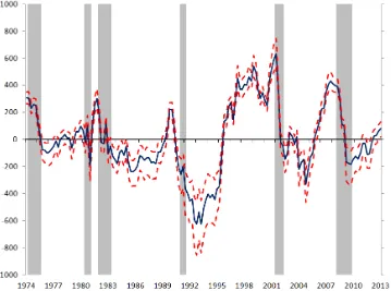
We rst describe the time variations that our model delivers. In gure 1.3 we report the highest68percent posterior tunnel for the variability of the monetary policy shock and in gure 1.4 the highest68percent posterior tunnel for the non-zero contemporaneous structural parameters t:

There are signi cant changes in the standard deviation of the policy shocks and a large swing in the late 1970s-early 1980s is visible. Given the identi ca-tion restricca-tions, this increase in volatility must be attributed to some unusual and unexpected policy action, which made the typical relationship between interest rates and money growth different. This pattern is consistent with the arguments of Strongin (1995) and Bernanke and Mihov (1998b), who claim that monetary policy in the 1980s was run differently, and agrees with the results of Sims and Zha (2006).

Figure 1.4 indicates that the non-policy parameters[ 1;t; 2;t; 5;t]exhibit

con-siderable time variations which are a posteriori signi cant. Note that it is not only the magnitude that changes; the sign of the posterior tunnel is also affected. Also worth noting is the fact that both the GDP coef cient in the in ation equation ( 1;t) and the in ation coef cient in the unemployment equation ( 5;t) change

sign, suggesting a generic sign switch in the slope in the Phillips curve.

The parameter 11;t, which controls the reaction of the nominal interest rates

to money growth, also displays considerable changes. In particular, while in the 1970s and in the rst half of the 1980s the coef cient was generally small and at times insigni cant, it becomes much stronger in the rest of our sample (1986-2005). Interestingly this time period coincides with the Greenspan era, where of-cial statements claimed that monetary policy was conducted using interest rates as instruments and money aggregates were endogenous.

The coef cients of the money demand equation, [ 3;t; 6;t; 9;t]0 are also

un-stable. For example, the elasticity of money demand to the nominal interest rate ( 9;t)is negative at the beginning of the sample and turns positive since the middle

(48)

Figure 1.3: Median and posterior 68 percent tunnel, volatility of monetary policy shock.

Also interesting is the fact that the elasticity of money (growth) demand to in a-tion is low and sometimes insigni cant, but increasing in the last decade. Thus, homogeneity of degree one of money in prices does not hold for a large portion of our sample.

One additional features of gure 1.4 needs to be mentioned. Time variations in elements of t are correlated (see, in particular, 5;t and 8;t or 1t and 11t).

Thus our setup captures the idea that policy and private sector parameters move together.

In sum, in agreement with the DSGE evidence of Justiniano and Primiceri (2008) and Canova and Ferroni (2012), time variations appear in the variance of the monetary policy shock and in the contemporaneous policy and non-policy coef cients.

1.5.6 The transmission of monetary policy shocks

We study how the time variations we have described affect the transmission of monetary policy shocks. Since mp

t is time-varying, we normalize the impulse

(49)

Figure 1.4: Estimates of

In theory, a surprise increase in the monetary policy instrument, should make money growth, output growth and in ation fall, while unemployment should go up. Such a pattern is present in the data in the early part of the sample, but dis-appears as time goes by. As gure 1.5 indicates, monetary policy shocks have the largest effects in 1981; the pattern is similar but weaker in 1975 and 1990. In 2005, prices, output and unemployment effects are perverse (in ation and out-put growth signi cantly increase and unemployment signi cantly falls after an interest rate increase). Note that the differences in the responses of output and unemployment between, say, 1981 and 2005 are a-posteriori signi cant. Thus, it appears that the ability of monetary policy to affect the real economy has consid-erably weakened over time and policy surprises are interpreted in different ways across decades.

(50)

Figure 1.5: Dynamics following a monetary policy shock, different dates.

(51)

1975 1981

[image:51.595.101.479.144.417.2]

1990 2005

Figure 1.7: Time varying and time invariant responses.

Our results are very much in line with those of Canova et al. (2008), even though they use sign restrictions to extract structural shocks, and of Boivin and Giannoni (2006), who use sub-sample analysis to make their points. They differ somewhat from those reported in Sims and Zha (2006), primarily because they do not allow for time variations in the instantaneous coef cients, and from those in Fernández-Villaverde et al. (2010), who allow for stochastic volatility and time variations only in the coef cients of the policy rule.

1.5.7 A time invariant over-identi ed model

We compare our results with those obtained in a constant coef cient overidenti ed structural model. Given that time variations seem relevant, we would like to know how the interpretation of the evidence would change if one estimates a model with

xed coef cients.

(52)

(1975, 1981, 1990, 2005). Clearly, there is more uncertainty regarding the liquid-ity effect in the time varying SVAR model at some dates. Furthermore, the re-sponses of output growth, in ation and unemployment in the constant coef cients model are different and the dynamics prevailing in the 1970s seem to dominate. Thus, the two systems give quite a different interpretation of the transmission of monetary policy shocks.

1.6 Conclusions

This paper proposes a uni ed framework to estimate structural VARs. The meth-odology can handle time varying coef cient or time invariant models, identi ed with recursive or non-recursive restrictions, that are just identi ed or overidenti-ed, and where the restrictions are of linear or non-linear type. Our algorithm adds a Metropolis step to a standard Gibbs sampling routine but nests the model into a general non-linear state space. Thus, we greatly expand the set of structural VAR models that researchers can deal with within the same estimation framework.

We apply the methodology to the estimation of a monetary policy shock in a non-recursive overidenti ed TVC model similar to the one used by Robertson and Tallman (2001), Waggoner and Zha (2003) with xed coef cients. In the context of this example, we examine the merits of multi-move vs. a single move routines and nd that once data are standardized, the computational costs of using a single-move routine are larger than the ef ciency gains. We show that there are important time variations in the variance of the monetary policy shock and in the estimated non-zero contemporaneous relationships. These time variations translate in im-portant changes in the transmission of monetary policy shocks to the variables in the economy. We also show that a different characterization of the dynamics in response to monetary policy shocks would emerge in an overidenti ed but xed coef cient VAR.

(53)

Chapter 2 MEASURING THE STANCE OF

MONETARY POLICY IN A

TIME-VARYING WORLD

2.1 Introduction

The stance of monetary policy is of general interest for macroeconomists and the private sector. It provides an important input to understand the current state of the economy and contributes to the expectations formation of future states. Despite its importance, it has been dif cult to have an exact measure of this stance, given the lack of consensus on what were the instruments of monetary policy and operating procedures at each point in time. Currently, this task has turned even more dif -cult after the introduction of so-called Unconventional Monetary Policies (UMP) and the achievement of the Zero-Lower-Bound (ZLB) of the Federal Funds Rate (FFR), given that the latter used to be considered the core instrument at least for the last two decades. The purpose of this paper is to provide a measure of the policy stance which takes into account changes in the operating procedures of the Fed.