An improved ant colony algorithm for the job shop scheduling problem

An improved ant colony algorithm for the Job Shop

Scheduling Problem

Guillermo Leguizam ´on

LIDIC - Departamento de Inform´atica

Universidad Nacional de San Luis

Ej´ercito de los Andes 950

5700 San Luis, Argentina

legui@unsl.edu.ar

Martin Sch ¨utz

NuTech Solutions GmbH

Martin-Schmeisser-Weg 15

44227 Dortmund, Germany

martin.schuetz@nutechsolutions.de

Abstract

Instances of static scheduling problems can be easily represented as graphs where each node represents a particular operation. This property makes the Ant Colony Algorithms well suited for different kinds of scheduling problems. In this paper we present an improved Ant System for solving the Job Shop Scheduling (JSS) Problem. After each cycle the Ant System applies a scheduler builder to each solution. The schedule builder is able to generate under a controlled manner different types of schedules (from non-delay to active). Any improvement achieved for a solution will affect the performance of the algorithm in the next cycles by changing accordingly the amount of pheromone on certain paths. Since the pheromone is the building block of an ant algorithm, it is expected that these changes guide the search towards more promising areas of the search space.

The computational study involves a set of instances of different size and difficulty. The results are compared against the best solutions known so far and results reported from earlier studies of ant algorithms applied to the JSSP.

Keywords: ant colony optimization, job shop scheduling problem, active and non-delay schedules.

1

Introduction

The Ant Colony Optimization (ACO) technique has emerged recently (Dorigo et al. [6, 7, 11]) as a new meta-heuristic for hard combinatorial optimization problems. ACO algorithms, that is, instances of the ACO meta-heuristics, are basically a multi-agent system where low level interactions between single agents (called artificial ants) result in a complex behavior of the whole system. ACO algorithms have been inspired by colonies of real ants [6], which deposit a chemical substance (calledpheromone) on the ground. This substance influences the choices ants make: the larger the amount of pheromone on a particular path, the larger the probability that an ant selects the path. Artificial ants, in ACO algorithms, behave in a similar way.

✁

Early experiments with ACO algorithms were devoted to ordering problems such as the Traveling Salesperson Problem [7,8], the Quadratic Assignment Problem [9], as well as the Job Shop Schedul-ing, Vehicle RoutSchedul-ing, Graph Coloring and Telecommunication Network Problem [6]. More recently, promising results were reported in [5, 12,4] from the application of a new version of an Ant System to the Multiple Knapsack and Maximum Independent Set Problem.

So far, there exist a few applications of the ACO approach to scheduling problems. Dorigo et al. [10,11] and Zwaan et al. [18] reported some promising results for the Job Shop Scheduling prob-lem. St¨utzle [16] developed an efficient ACO approach for solving the Flow Shop Problem by in-cluding a local search technique. St¨utzle et al. [17], Bauer et al. [1], and Merkle et al. [13] proposed different ant algorithms for the Single Machine Total Weighted Tardiness Problem. The results pre-sented in [13, 15] were obtained from the application of an ant algorithm that includes a technique which allows the ants to take into account pheromone values that have already been used for earlier decisions. In a more recent work Merkle et al. [14] proposed a novel approach for evaluating the pheromone. He applied this new approach, which is a combination of two pheromone evaluation methods, to the resource constrained project scheduling problem.

It is important to note that ACO algorithms can be directly applied to discrete optimization prob-lems that can be characterized as a graph ✂✁☎✄✝✆✟✞✡✠☞☛

. Here, ✆

denotes a finite set of components

and

✠✍✌✎✆✑✏✒✆

the set ofconnectionsbetween the components (see [6] for a complete description). Each solution of the optimization problem may be expressed in terms of feasible paths on the graph . Thus, ACO algorithms can be used to find minimum cost paths (sequences) feasible with respect to the constraint set✓

1_.

In ACO algorithms a population (colony) of agents (ants) collectively solves the optimization problem under consideration by using the above graph representation. Information collected by the ants during the search process is encoded with the help ofpheromone trails✔✖✕✗ associated with

con-nection

✄✙✘✚✞✜✛✢☛

. Pheromone trails encode a long-term memory about the whole ant search process. Depending on the problem representation chosen, pheromone trails may be associated with all arcs, or only with some of them. Arcs can also have an associatedheuristic value✣✤✕✗ representinga priori

information about the problem instance or run-time information provided by a source different from the ants.

In this paper we consider the application of the ACO approach for the Job Shop Scheduling Problem. The study is focused on the covered area of the search space regarding non-delay and active schedules and the influence of the covered area on the overall performance of the algorithm. Additionally an alternative heursitic value ✣✥✕✗ is considered for the probability item selection. The

rest of the paper is organized as follows. In section 1 we illustrate the basic concepts of the Job Shop Scheduling Problem, section2presents a brief discussion about different types of schedules and the respective hierarchical relationship between them. The Ant System for the JSSP similar to the original proposal (AS-JSS) and our proposal for the present work (AS-JSS-✦ ) are shown in section3.

AS-JSS-✦ introduces a phase to obtain an active schedule from a permutation possibly representing a

semi-active one. Section4describes the experiments and corresponding results from the application of AS-JSS and AS-JSS-✦ to a set of different instances of the JSSP. The conclusion and outlook for

future studies are presented in section6.

1_{For example, in the traveling salesperson problem}

✧ is the set of cities,★ is the set of arcs connecting cities, and✩

2

General formulation of the JSSP

The JSSP consists of a finite set of✁ jobs✂✄ ✕✆☎✞✝

✕✠✟☛✡ to be processed on a finite set

☞ of✌ machines ✂✍☞✏✎✑☎✞✒

✎✓✟☛✡ . Each job

✕ must be processed on every machine and consists of a chain of✌ ✕ operations

✔

✕✕✡

✞

✔

✕✗✖ ✞✙✘✚✘✚✘✞

✔

✕

✒✜✛

which have to be scheduled in a predetermined given order (precedence constraint). There are ✢

✁✤✣

✝

✕✠✟☛✡

✌ ✕ operations in total where

✔

✕✗✎ is the operation of job ✕ which has to be

processed on machine☞✥✎ for an uninterrupted processing time✦ ✕✗✎ . No operation may be pre-empted.

Each job has its own individual flow pattern through the machines which is independent of the other jobs. Each machine can process only one job and each job can be processed by only one machine at a time (capacity constraints). The duration in which all operations for all jobs are completed is referred to as the makespan ✆

✒✜✧✩★

. Our objective here is to determine the starting times (✪ ✕✗✎✬✫✮✭ ) for each

operation, in order to mininise the makespan while satisfying all constraints:

✆✰✯

✒✜✧✩★

✁

✌

✘

✁✱✂

✆

✒✜✧✩★

☎

✁

✌

✘

✁

feasible schedules

✂✍✲✴✳✍✵✶✂✞✪✜✕✗✎✸✷✹✦ ✕✗✎✑☎✻✺✑✼✽ ✕✱✾✬

✞

✼✿☞✏✎❀✾❁☞✤☎

The dimensionality of each JSSP instance is specified as ✁

✏

✌ and ✢ is often assumed to be

✁

✏

✌ provided that✌ ✕

✁

✌ for each job ✕❂✾❃ and each job has to be processed exactly once on

each machine. In a more general statement2_{of the job shop problem, machine repetitions (or machine}

absence) are allowed in the given order of the job ☞✕❄✾❅ , and thus✌ ✕ may be greater (or smaller)

than✌ .

3

Types of schedules

The encoding of problem solutions should ensure that all possible solutions can be generated, oth-erwise the algorithm could fail to reach an optimal solution due to an inappropriate representation. However, ant algorithms do not process a complete (encoded) solution as in most local search tech-niques. Instead, they build the schedules in a manner that not necessarily all possible schedules can be generated (more details in section4). Therefore, this is an important issue when the set of all pos-sible schedules is considered regarding the search space. According to the schedule properties, there exist four cases for any feasible schedule: inadmissible, semi-active, active, and non-delay schedules. Figure1shows the respective relationships.

semi−active active non−delay

optimal schedules inadmissible

Figure 1: Hierarchy of feasible schedules.

The number of inadmissible schedules is infinite and most of them contain excessive idle times. A semi-active schedule can be obtained by forward-shifting a schedule until no such excessive idle times

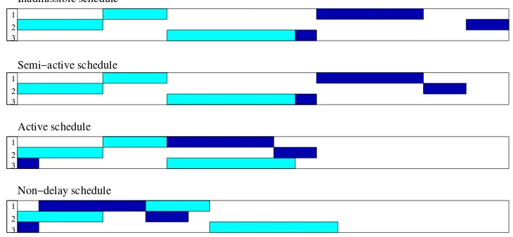
2

exist. Further improvements on asemi-active schedule can be reached by skipping some operations to the front without causing other operations to start later regarding the original schedule. However, active schedules allows no such shift. Thus the optimal schedule is guaranteed to fall within the active schedules. Non-delay schedules build a subset of active schedules. In a non-delay schedule, a machine is never kept idle if some operation is able to be processed. Is important to note that the best schedule is not necessarily non-delay. However, a non-delay schedule is easier to generate than active schedules and may be a very near optimal schedule even if it is not an optimal one. Additionally, there is strong empirical evidence that non-delay schedules show a better mean solution quality that active ones. Nevertheless, typical scheduling algorithms search the space of active schedules in order to guarantee that the optimum is taken into consideration. Figure2shows four different schedules for the same instance of the JSSP where each of them respectively fits the classification given above.

1 2 3

1 2 3

1 2 3

1 2 3

Semi−active schedule Inadmissible schedule

Active schedule

Non−delay schedule

Figure 2: Four different schedules for a particular instance with✌ ✁✁

machines and✁ ✁✄✂

jobs.

When generating a schedule, the most common way is to choose an operation from a set of schedulable operations one at time and assign a start time to each. A schedulable operation is an operation all of whose preceding operations have been completed. The problem is how to choose an operation from the set of schedulable operations and how to assign the start time to this operation.

It is worth remarking that a solution built by each ant represents a permutation☎

✁ ✄

✦✱✡

✞

✦ ✖ ✞✙✘✚✘✚✘✞

✦

✝✝✆✑✒

) of operations where✦✟✞ indicates a unique operation ✠ for a particular job

✘

(✔

✕✗✎ ). Each job

✘

defines a production recipe ✡ ✕ given as an order of the machines it has to pass. The vector ✡ ✕ points to the

machines, hence for✡ ✕

✄

✠

☛ ✁ ✛ ✄☞☛✍✌ ✛✎✌

✌ ✕

☛

machine

✛

is the✠ -th machine that processes job

✘

. In general, a permutation ☎ can be decoded as an semi-active, active or non-delay schedule.

However, as we pointed out above, the optimal schedules are active (which includes the non-delay schedules) but no necessarily non-delay. Accordingly to the above definition semi-active schedules can be improved to obtain an active one by shifting some operations.

The schedule builder in Figure3(taken from [3]) generates active and non-delay schedules from a permutation of operations. The parameter✦ (✭

✌

✦

✌✏☛

) controls the type of schedule to be generated. Thus, non-delay schedules are obtained by setting ✦

✁

✭ , all active schedules can be generated with

✦

✁✑☛

1. Build the set of all beginning operations, ✂✁☎✄✝✆ ✕✕✡✟✞✠☛✡✌☞✍✡✌✎✑✏ .

2. Determine an operation ✆✓✒ from with the earliest possible completion time,✔✖✕✝✗✙✘✚✕

✡

✔ ✕✗✎✛✗✙✘✢✕✗✎

for all✆ ✕✗✎✢✜✣ .

3. Determine the machine✤✥✕ of✆✓✕ and build the set✦ from all operations in which are processed

on✤✂✕,✦✧✁☎✄✝✆ ✕✗✎✢✜✣ ✞★ ✕✪✩✬✫✮✭ ✁✯✤✂✕✏ .

4. Determine an operation ✆✰✕✕ from ✦ with the earliest possible starting time, ✔✱✕✕✲✁✳✔ ✕✗✎ for all

✆ ✕✗✎✢✜✣✦ .

5. Delete operations in✦ in accordance to parameter✴ such that✦✧✁☎✄✝✆ ✕✗✎✢✜✣✦ ✞✔ ✕✗✎✢✵✶✔✷✕✕✓✗✸✴ ✩✹✩ ✔✷✕✟✗

✘✚✕✭✻✺ ✔✷✕✕✭✪✏ .

6. Select the operations ✆

✯

✕✗✎ from

✦ which occurs leftmost in the permutation and delete it from

(i.e.,✥✼✁✽✿✾❀✄✝✆

✯

✕✗✎ ✏ ).

7. Append operation✆

✯

✕✗✎ to the schedule and calculate its starting time.

8. If a job succesor operation✆

✯

✕❂❁✎❄❃☛✡ of the selected operation

✆

✯

✕✗✎ exists, insert it into .

9. If❆❅✁✯❇ , goto Step 2, else terminate.

Figure 3: Hybrid schedule builder based on parameter✦ .

4

Ant System for the JSSP

In this section we show an Ant Colony algorithm for the JSSP. Classical descriptions of ACO algo-rithms are basically related to the Travelling Salesperson Problem3_{. The description presented here}

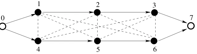
is based on ealier work done for scheduling problems by applying the ACO approach [10, 11, 18]. Basically, an instance of the JSSP in the ACO algorithm is represented as a graph where the nodes are connected by two kind of edges. The directed edges which represent the precedence between opera-tions for the same job and the undirected edges representing possible path to follow by the ants if the problem constraints are satisfied. The graph in Figure4represents a JSSP instance with✁

✁

jobs and✌

✁ ✂

machines. Each node represents an operation. Thus, node ☛

represents the first operation of job

☛

, node

✂

the second operation and so on. In general, node

✘ represents the ✄✙✘ mod ✄ ✌ ✷ ☛✖☛✚☛ -th operation of job ✄✙✘

div ✄

✌ ✷

☛✖☛✚☛

✷

☛

. Nodes ✭ and

✄

✁

✏

✌ ✷

☛✖☛

are dummy operations which repre-sent respectively the starting and final nodes in the path that each ant builds. Consequently each ant that tries to find a schedule for a JSS instance will start from node ✭ and then visit all nodes either

following dependencies edges (directed) or undirected edges (if the problem constraints are satisfied). For example, the sequence of operations✦

✁ ✄

✭

✞ ☛✥✞✖❈ ✞❊❉✢✞ ✂✢✞ ✞❄❋ ✞❊●✥☛

is a possible feasible solution for the instance in Figure4. Each ant builds a solution ”walking” from node ✭ to node

●

by visiting all nodes, i.e., scheduling each operation to complete the schedule. The decision about the path will depend on the values of the pheromone laid on the connections and the corresponding heuristic values. Thus, the variables✔ ✕✗

✄

✪

☛

denotating the intensity of pheromone on connection

✄✙✘✚✞✜✛✢☛

at time✪

are defined as

✔ ✕✗ ✄ ✪✽✷ ☛✖☛ ✁ ✄☞☛☛❍✽■✢☛ ✔ ✕✗ ✄ ✪ ☛ ✷☎❏ ✔ ✕✗ ✄ ✪ ☛ ✞ (1) where ✭✥❑ ■ ✌ ☛

is a coefficient representing pheromone evaporation. ❏ ✔ ✕✗

✄ ✪ ☛ ✁✥✣ ✧▲ ✟☛✡ ❏ ✔ ▲ ✕✗ ✄ ✪ ☛ ,

2 3

4 5 6

7 0

1

Figure 4: Instance of JSS represented as a graph.

where is the actual number of ants in the colony and❏ ✔

▲

✕✗

✄

✪

☛

is the quantity per unit of length of trail substance (pheromone for real ants) laid on connection

✄✙✘✚✞✜✛✢☛

by the ✁ -thant at time✪ and is given by

the following formula:

❏ ✔ ▲ ✕✗ ✄ ✪ ☛ ✁ ✂☎✄

✆✞✝ if e-thant uses edge (i,j) on its sequence of operations ✭ otherwise.

(2)

Here, ✟ is a constant and

✠

▲ the makespan found by the

✁ -th ant. For each edge, the intensity of

pheromone at time 0 (✔ ✕✗

✄

✭

☛

) is set to a very small value. An alternative way of getting❏ ✔ ✕✗

✄

✪

☛

is con-sidering only the best ant in the current cycle instead of all ants in the colony. By this elitist approach, only the connections involved in the best solution will be affected regarding the reinforcement of the pheromone level. In this case, ❏ ✔ ✕✗

✄ ✪ ☛ ✁ ❏ ✔ ▲ ✕✗ ✄ ✪ ☛

, where✁ ✾ ✂

☛✥✞✙✘✙✘✙✘ ✞

☎ is the index of the ant that

found the best solution in the current cycle of the algorithm.

While building a permutation of operations, the probability that ant ✁ schedules operation

✛

pro-vided that✘

was the last operation scheduled by ant ✁ is given by

☎ ▲ ✕✗ ✄ ✪ ☛ ✁✡✠ ☛☞ ✛✌✎✍✏✒✑✔✓✕ ☛✖ ✛✌✗✓✘ ✙✛✚✢✜✤✣ ✝✦✥✧✩★ ☛☞ ✛ ✚ ✍✏✒✑✔✓ ✕ ☛✖ ✛ ✚ ✓ ✘ ✞ if✛ ✾✫✪ ▲ ✄ ✪ ☛ ✭ ✞ otherwise, (3) where ✪ ▲ ✄ ✪ ☛

is the set of schedulable operation still not scheduled by ant ✁ at time ✪ , and ✣ ✕✗

✄

✪

☛

represents the visibility or local heuristic. There exist different priority rules that have been proposed in the literature, however none of then dominates all the others. Our heuristic value which is different from that considered in [10, 11, 18], is calculated as ✣ ✕✗

✄ ✪ ☛ ✁ ☛✭✬ ✄✝✆ ✪ ✘ ✌✮✁✡✗ ❍✰✯ ✪ ✘ ✌✮✁✡✗ ☛ . ✆ ✪ ✘ ✌✮✁✡✗ and ✯ ✪ ✘

✌✮✁✡✗ represent respectively the completion of operation

✛

and the period of time that a particular machine stays idle due to assignation of operation✛

. The rationale behind this heuristic value is that scheduleable operations that finish as early as possible and avoid idleness of a particular machine are preferable. Thus, the smaller

✆

✪

✘

✌✮✁ ✗ and

✯

✪

✘

✌✮✁✡✗ , the higher is the heuristic value associated to

operation✛

.

The parameters ✱ and ✲ control the relative importance of pheromone versus visibility (local

heuristic). Hence, the transition probability is a trade-off between visibility, which says that operations finishing earlier should be chosen with a higher probability, and trail intensity associated to connection

✄✙✘✚✞✜✛✢☛

representing the learned desirability of choosing operation✛

immediately after operation✘

. A data structure, called a tabu list, is associated to each ant in order to avoid that ants schedule operations already scheduled. This list✪✳✵✴✤✶

▲

✄

✪

☛

maintains a set of scheduled operations up to time ✪

for the ✁ -th ant. When a solution is completed, the list✪✳✵✴✤✶

▲ ✄ ✪ ☛☞✄ ✁ ✁✑☛✥✞✙✘✚✘✞ ☛

is emptied and every ant is free again to choose an alternative permutation of operations for the next cycle.

1. initialize

2.for✔✛✁ ✠ tonumber of cyclesdo

3. for ✁ ✠ to✁ do

4. ✘ ✁ ✩

✂

✭ / / The permutation starts with the dummy operation

5. ✄

▲

✁☎✄✝✆ ✞✆ is the first operation from each job✏

6. repeatuntil✄

▲ is empty

7. ✘ ✵☛✵ select operation☎ to be incorporated with prob. ✆

▲

✕✗ given by Eq. (3)

8. ✄

▲

✁✝✄

▲

✺ ✄✞☎ ✏✠✟☛✡ ✄✌☞ ✩ ✎✍✏☎ ✭

9. end 10. calculate✑

▲

, the cost of✘ (the generated solution)

11. save the best solution so far 12. end

13. updatethe trail levels✒

✕✗ on all paths according to Eq.(1)

14.end

15. print the best solution found

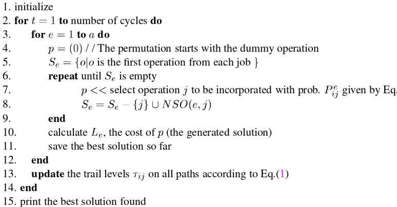
Figure 5: General outline of an Ant System for the Job Shop Scheduling Problem(AS-JSS).

the dummy operation. When all ants have completed a solution, the pheromone is deposited on the connections (off line approach). The ant algorithm iterates for a pre-determined number of cycles. Within each cycle, each ant builds a permutation of operations that represents the order in which the operations have to be scheduled. The index ✘

in line ●

represents the last operation scheduled, i.e., the last operation in the partial permutation being built. The operation

✛

is selected under the roulette wheel mechanism proportional to the probability ☎

▲

✕✗ .

✢✔✓✠✕ is a function returning a single set of

possibly the next schedulable operation or the empty set if no operation remains to be scheduled. Thus, each ant can be seen as a schedule builder where the decision concerning the selection of the next operation to be scheduled is based on the global information (amount of pheromone) and the heuristic value calculated with the help of

✆

✪

✘

✌✮✁ and

✯

✪

✘

✌✮✁ . It is interesting to note that working

in this way the colony represents several iterative schedule builder working in parallel and sharing some global information. The ants (schedule builder) build semi-active schedules due to the fact that all operations are scheduleable as long as they satisfy the problem constraints, however, no additional constraints are considered from which non-delay or active schedules could be obtained.

Our approach aims not at controlling the type of schedules that the ants obtain, instead, it aims at processing the solutions or permutation found in each cycle. The AS-JSS-✦ algorithm is similar

to AS-JSS (algorithm in Figure5) except that between lines✖ and

☛

✭ , the Hybrid Scheduler Builder

(HSB) described in Figure 3 is integrated aiming at the improvement of the solutions found so far. The application of✗✘✓✠✙ is biased according to a special parameter called✦ . Thus, any improvement

on some solution could influence the pheromone laid on the paths involved in the solution. ✗✘✓✠✙

receives a permutation obtained for a particular ant and then builds a new one by applying the steps described in Figure3.

5

Experiments and Results

We studied the performance of AS-JSS and AS-JSS-✦ applied to several instances of the Job Shop

Scheduling problem. The instances considered were taken from the OR Library [2]. They include a set of well known problems where some of them were considered here. The parameters for AS-JSS are ✱

✁ ☛

, ✲

✁ ❉

, ✁

✭ , and

■ ✁

✭

✘❉

. For AS-JSS-✦ the parameters are ✱

✁ ☛

, ✲

✁ ☛

, ✁

✭ , and ✦ ✾ ✂✑✭ ✭ ✭ ✭ ✭ ✭ ✖ ☎ . The number of cycles for both versions of the ant

system was set to ✭ ✭ ✭ . AS-JSS and AS-JSS-✦ were run

☛

✭ times using different random seeds for

each instance considered. For both algorithms,✟ (cf. Eq.2) was set to the best known value of the

respective instance.

The next section shows the influence of ✦ on the performance of AS-JSS-✦ . In section 5.2 we

make a comparison considering the best results from the application of AS-JSS and AS-JSS-✦ . Also,

some considerations are made with respect to the results obtained in the earlier applications of the ACO approach to JSS.

All tables express the results as the percentage error from the best known solution and the respec-tive average error over the

☛

✭ runs (between parenthesis).

5.1

Influence of parameter

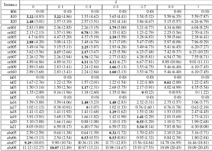
The influence of the parameter ✦ on the performance of the ant algorithm is sketched in Table 1

where the results from the different values of ✦ ✾ ✂✑✭

✞

✭

✘☛✥✞

✭

✘ ✞

✭

✘❉✢✞

✭

✘●✢✞

✭

✘

✖

✞ ☛

☎ are shown. Clearly, the

best (and most robust) performance of AS-JSS-✦ is in correspondence with ✦

✁

✭

✘

and ✦

✁

✭

✘❉

, except for ft10, ft20, orb04, and abz7 for which setting ✦

✁

✭ obtained the best results. Also, it is

important to note the tendency that the error increases as the value of✦ gets closer to

☛

. However, for some instances tested (la02, la04, la19, la20, la21) AS-JSS-✦ obtained the best results using✦

✁

✭

✘

✖ ,

✦

✁

✭

✘●

, ✦

✁

✭

✘●

, ✦

✁

✭

✘●

, and ✦

✁

✭

✘●

respectively. As we can observe, there is a strong evidence that✦

✁

✭

✘

and✭ ✘❉

builds a robust region of the search space.

Instance ✁

✂ ✂☎✄

✡

✂☎✄✆ ✂☎✄✝ ✂☎✄✞ ✂☎✄✟

✡

ft06 0 (0) 0 (0) 0 (0) 0 (0) 0 (0) 0 (0) 0 (0)

ft10 3.22(4.93) 3.22(4.86) 3.33 (4.62) 3.65 (4.41) 3.54 (5.32) 5.59 (6.35) 5.59 (7.87) ft20 2.48(3.01) 2.57 (3.10) 2.57 (3.51) 2.91 (4.14) 3.86 (4.67) 5.15 (5.57) 6.26 (6.79) orb01 2.83 (3.89) 2.36 (2.85) 2.26 (3.15) 1.79(3.00) 3.21 (4.77) 4.34 (6.00) 6.04 (8.25) orb02 2.13 (2.13) 1.57 (1.98) 0.78(1.38) 1.35 (1.82) 1.23 (2.79) 2.25 (3.56) 2.70 (4.15) orb03 4.7 (6.93) 4.47 (5.20) 4.37 (5.19) 2.18(3.59) 3.28 (4.83) 3.58 (5.66) 2.38 (6.41) orb04 2.88(4.20) 3.08 (4.12) 3.48 (4.74) 5.17 (7.05) 5.47 (7.05) 5.97 (8.08) 7.96 (9.29) orb05 3.49 (4.74) 3.15 (5.11) 2.25(3.87) 2.93 (4.28) 3.49 (4.73) 5.41 (6.45) 6.20 (7.27) orb06 3.62 (3.56) 2.17(2.66) 2.17(3.67) 4.25 (5.58) 6.23 (7.48) 7.42 (9.37) 6.23 (10.25) orb07 2.26 (2.79) 2.26 (2.94) 1.76(2.74) 2.77 (3.82) 4.28 (5.81) 6.54 (7.78) 7.55 (8.71) orb08 4.89 (6.86) 4.89 (6.31) 4.11(6.32) 4.11(6.27) 6.67 (7.81) 8.89 (10.86) 9.01 (11.11) orb09 2.89 (3.68) 2.83 (3.41) 2.24 (2.84) 1.66(3.13) 3.53 (4.75) 5.46 (6.40) 6.10 (7.45) orb10 2.89 (3.68) 2.83 (3.41) 2.24 (2.84) 1.60(3.13) 3.53 (4.75) 5.46 (6.40) 6.10 (7.45)

la01 0 (0) 0 (0) 0 (0) 0 (0) 0 (0) 0 (0) 0 (0)

la02 1.67 (2.76) 1.22 (2.70) 1.57 (2.01) 1.22 (1.54) 1.22 (1.80) 0.61(2.00) 1.22 (2.45) la03 1.50 (3.14) 1.50 (2.56) 1.17(2.31) 2.68 (3.75) 2.17 (3.91) 4.02 (4.99) 4.35 (5.54) la04 1.35 (2.00) 0.16 (1.96) 1.18 (2.60) 1.35 (1.96) 0(0.22) 0 (0.93) 0 ( 1.22)

la05 0 (0) 0 (0) 0 (0) 0 (0) 0 (0) 0 (0) 0 (0)

la16 3.59 (3.88) 3.59 (4.06) 1.48(3.23) 1.48(2.83) 2.32 (3.31) 2.75 (3.57) 3.06 (3.77) la17 1.02 (1.13) 0.38 (0.91) 0(1.07) 1.02 (1.33) 0.76 (1.60 ) 0.76 (1.78) 0.63 (2.19) la18 1.41 (1.42) 1.41 (1.92) 1.41 (1.68) 1.29(1.62) 1.53 (2.18) 1.53 (3.03) 2.47 (4.45) la19 3.91 (3.91) 3.68 (3.78) 1.66 (1.82) 1.42 (1.99) 1.41(2.29) 2.01 (3.69) 2.73 (4.21) la20 3.10 (3.88) 1.66 (1.66) 0.88 (1.08) 1.10 (1.15) 0.55(1.29) 1.10 (1.71) 1.99 (2.68) la21 8.03 (9.01) 6.59 (8.17) 6.40 (7.76) 6.59 (7.32) 5.54(8.14) 7.83 (8.56) 6.30 (8.08) abz05 2.59 (2.59) 0.64 (1.38) 0.64 (1.39) 0.32(1.72) 1.70 (2.43) 2.10 (3.24) 3.16 (3.71) abz06 2.96 (3.13) 2.54 (2.54) 0.53(0.53) 0.53(0.81) 0.95 (1.32) 0.84 (2.39) 1.80 (2.84) abz07 9.29(10.03) 9.90 (10.74) 10.36 (11.18) 11.73 (12.83) 13.56 (14.84) 14.78 (16.95) 16.46 (18.81) abz08 11.12 (12.27) 10.07(12.49) 10.97 (13.21) 13.98 (14.67) 15.93 (17.53) 19.09 (20.45) 19.09 (20.45)

Table 1: Results from AS-JSS-✦ by using different values of✦ .

Also, it is important to note that for some instances, the variation of the values of✦ does not affect

value was found in all cases. Clearly, a larger value of ✦ (e.g., ✭ , ✭ ✖ , and ) increases the search

space and for some instances the performance ofAS-JSS-✦ decays, however, for instances la02, la04,

and la19-21, a large value of ✦ let the algorithm obtain the best results. The worst performance of

AS-JSS-✦ was obtained on instances abz07 and abz08. Nevertheless, the qualitative difference of the

results is remarkable when the algorithm searches (or near) the set of non-delay schedules (✦

✁

✭

✞

✭

✘☛

) instead of the set of active schedules (✦✁

☛

).

5.2

Comparison between AS-JSS and

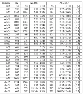
AS-JSS-In this section we compare the performance of AS-JSS-✦ and AS-JSS (the version of the ant system

that implicitly searches on the set of semi-active schedules). Table2shows four columns denoting the following: the instances tested, the best known value (BK) , and the results from AS-JSS and

AS-JSS-✦ respectively. For each version of the ant algorithm, the best found value and minimum error (with the

average minimum error) are displayed. Additionally, a third column for AS-JSS-✦ shows the setting

of the parameter✦ from which the best result was obtained. The set ✂

❍

☎ means that for all values of ✦ the same result was obtained (see ft06, la01, and la05). Regarding the search space considered by,

either AS-JSS or AS-JSS-✦ , it is worth remarking that for some instances, both algorithms were able

to find the same results (ft06, ft20, ob05, la01, la04, la05, and la19) or similar results (orb05, orb08, la02, la20, and abz06). For the first group, except for ft20, ob05, and la19, the algorithms found the best known values. Because the instances mentioned above are not the hardest, the algorithms converged to good quality solutions independently of the size of the search space considered (non-delay to semi-active). However, an important benefit was obtained when the size of the search space to be considered was controled through different values of✦ . See instances ft10, orb01-04, orb08-10,

la03, la16–la18, and la21. Also, abz07 and abz08 for which an important improvement on the quality of the results was obtained by bounding the search to the non-delay schedules. Finally, taking several runs into account, AS-JSS-✦ clearly offers a more robust behavior, except for ft06, la01, and la05.

6

Conclusions

In this paper we presented an approach to guide the ant system (AS-JJS-✦ ) to specific areas of the

search space in order to look for the optimal schedule. AS-JSS-✦ showed an improved perfomance in

comparison with AS-JSS on several test cases. Also it is important to note that AS-JSS and mainly AS-JSS-✦ performed better than the earlier versions of the ACO approach applied to JSS. According

to the results reported in [10,11], AS-JSS obtained a little bit higher value of the makespan only on the instance orb04. AS-JSS-✦ still generates semi-active schedules similarly to the earlier ant systems

for the JSS problem. The main difference is on the improving process applied to each solution found. This process changes the solution according to the parameter ✦ . The new solution found, if some

improvement is obtained, will influence the pheromone laid on the respective connections.

A proposal for a future work is considering the design of an Ant System which generates either, non-delay or active schedules controled by ✦ but during the construction phase. This could avoid an

Instance BK AS-JSS

AS-JSS-✁

ft06 55 55 0 (0) 55 0 (0) -✁

ft10 930 980 5.37 (6.23) 960 3.22 (4.93) 0✁

ft20 1165 1194 2.48 (3.37) 1194 2.48 (3.01) 0✁

orb01 1059 1095 3.39 (5.43) 1078 1.79 (3.00) 0.5✁

orb02 888 912 2.70 (3.20) 895 0.78 (1.38) 0.3✁

orb03 1005 1043 3.78 (6.20) 1027 2.18 (3.59) 0.5✁

orb04 1005 1088 8.25 (8.94) 1033 2.88 (4.20) 0✁

orb05 887 907 2.25 (5.42) 907 2.25 (3.87) 0.3✁

orb06 1010 1038 2.77 (3.87) 1032 2.17 (3.67) 0.3✁

orb07 397 409 3.02 (4.81) 404 1.76 (2.74) 0.3✁

orb08 899 944 5.00 (7.78) 936 4.11 (6.32) 0.3✁

orb09 934 978 4.71 (6.34) 949 1.60 (3.13) 0.5✁

orb10 944 982 4.02 (5.75) 962 1.90 (2.89) 0.3✁

la01 666 666 0 (0) 666 0 (0) -✁

la02 660 666 1.67 (1.67) 663 1.22 (1.54) 0.5✁

la03 597 634 6.19 (7.13) 604 1.17 (2.31) 0.3✁

la04 590 590 0 (1.93) 590 0 (0.22) 0.7✁

la05 593 593 0 (0) 593 0 (0) -✁

la16 945 979 3.59 (4.81) 959 1.48 (3.23) 0.3✁

la17 784 793 1.14 (1.98) 784 0 (1.07) 0.3✁

la18 848 868 2.35 (3.79) 859 1.29 (1.62) 0.5✁

la19 842 852 1.18 (1.91) 852 1.18 (2.29) 0.3✁

la20 902 911 0.99 (1.97) 907 0.55 91.29) 0.7✁

la21 1046 1127 7.74 (9.22) 1104 5.54 (8.14) 0.7✁

abz05 1234 1246 0.97 (1.81) 1238 0.32 (1.72) 0.5✁

abz06 943 954 1.37 (3.05) 948 0.53 (0.53) 0.3✁

abz07 656 775 18.14 (19.55) 717 9.29 (10.03) 0✁

abz08 665 787 18.34 (19.36) 732 10.07 (12.49) 0.3✁

Table 2: A comparison between the best values found byAS-JSS-✦ and AS-JSS.

References

[1] A. Bauer, B. Bullnheimer, R.F. Hartl, and C. Strauss. An ant colony optimization approach for the single machine total tardiness problem. InProceeding of the Congress on Evolutionary Computation, pages 1445–1450, 6-9 July, Whasington D.C., USA, 1999.

[2] J. E. Beasley. Or-library: distributing test problems by electronic mail.Journal of the Operations Research Society, pages 1069–1072, 1990.

[3] C. Bierwirth and D. Matffeld. Production scheduling and rescheduling with genetic algorithms.

Evolutionary Computation, 7(1):1–17, 1999.

[4] G. C. Leguizam´on and M. Sch¨utz. An ant system for the maximum independent set problem. InVII Congreso Argentino de Ciencias de la Computaci ´on, volume II, El Calafate, Santa Cruz, Argentina, 2001.

[5] M. Cena, M.L. Crespo, C. Kavka, and G. Leguizam´on. A Study of Performance of an Ant Colony System applied to Multiple Knapsack Problem. In E. Apayd, editor, Proceedings of EIS-98, pages 567–573. ICSC Academic, 1998.

[6] D. Cornea, M. Dorigo, and F. Glover, editors. New Ideas in Optimization. McGraw-Hill Inter-national, 1999.

[7] M. Dorigo, G. Di Caro, and L.M. Gambardella. Ant Algorithms for Discrete Optimization.

[8] M. Dorigo and L.M. Gambardella. Ant Colony System: A Cooperative Learning Approach to the Traveling Salesman Problem.IEEE Transactions on Evolutionary Computation, 1(1):53–66, 1997.

[9] M. Dorigo, V. Maniezzo, and A. Colorni. The Ant System Applied to the Quadratic Assignment Problem. Technical Report Technical Report IRIDIA 94/28, Universit´e Libre de Bruxelles, Belgium, 1994.

[10] M. Dorigo, V. Maniezzo, and A. Colorni. Ant System for thejob-shop scheduling. JORBEL -Belgian Journal of Operations Research, Statistics and Computer Science, pages 39–53, 1996.

[11] M. Dorigo, V. Maniezzo, and A. Colorni. The ant system: Optimization by a colony of cooper-ating agents. InIEEE Trasn. Systems, Man, and Cybernetics - Part B, pages 29–41, 1996.

[12] G. Leguizam´on and Z. Michalewicz. A New Version of Ant System for Subset Problems. In

Proceedings of the 1999 Congress on Evolutionary Computation, pages 1459–1464. IEEE Press, Piscataway, NJ, 1999.

[13] D. Merkle and M. Middendorf. An ant algorithm with a new pheromone evaluation rule for total tardiness problems. InProceeding of the EvoWorkshops 2000, number 1803 in Lectures Notes in Computer Science, pages 287–296. Springer Verlag, 2000.

[14] D. Merkle, M. Middendorf, and H. Schmeck. Ant colony optimization for resource constrained project scheduling. In D. Whiley et al., editor, Proceedings of the Genetic and Evolutionary Computation Conference (GECCO-2000), pages 893–900, Las Vegas, Nevada, USA, 10-12 July 2000. Morgan kaufmann.

[15] D. Merkle, M. Middendorf, and H. Schmeck. Pheromone evaluation in ant colony optimization, 2000. citeseer.nj.nec.com/merkle00pheromone.html.

[16] T. St¨utzle. An ant approach for the flow shop problem. In Proceedings of the 6th European Congress on Intelligent Techiniques & Soft Computing (EUFIT ’98), volume 3, pages 1560– 1564, Verlag, Aachen, 1998.

[17] T. St¨utzle, M.L. den Besten, and M. Dorigo. Ant colony optimization for the total weighted tardiness problem. In Parallel Problem Solving from Nature: 6th International Conference, volume 1917 of Lecture Notes in Computer Sciences, pages 611–620, Berlin, 2000. Springer Verlag.