THE GENDER WAGE GAP IN PERU 1986-2000:
EVIDENCE FROM A MATCHING COMPARISONS APPROACH1,2,3
HUGO ÑOPO 4
1.Introduction
Gender disparities in the Peruvian labor markets are pronounced. There are substantial gaps in participation and employment rates, in occupations, and in hourly wages and monthly earnings. While there are gender differences in these labor market outcomes, there are also gender disparities in individual characteristics. Males tend to have more years of education and longer tenure in higher paying occupations. The extent to which these differences in observable characteristics account for the gaps in labor market outcomes is a long-standing question. For the gender wage gap, the Blinder-Oaxaca decomposition has been the most popular approach in the labor market literature.5
The Blinder-Oaxaca decomposition is an algebraic manipulation of the differences between estimated Mincerian equations for males and females. It allows us to answer questions of the type: "What would the earnings of the average male (female) have been if his (her) observable characteristics had resembled those of the average female (male)?"
Ñopo (2004) develops a new methodology for the decompositions of wage gaps by introducing a matching comparisons approach. Matching males and females with the same observable individual characteristics generates synthetic samples of identical individuals. Then, the method allows us to answer questions of the type: "What would the earnings distribution of the sample of males (females) have been if their observable characteristics had resembled those of the sample of females (males)?" This extension garners immediate
1 JEL Classification: C14, D31, J16, O54.
Keywords: Matching, Non-parametric, Gender Wage Gap, Latin America.
2 Sections of this paper circulated previously under the title "Matching as a Tool to Decompose Wage
Gaps."
3 The advice of Chris Taber, Luojia Hu, and Dale Mortensen is deeply acknowledged. Sebastian Calónico,
Deidre Ciliento, Cristina Gomez and John Jessup provided valuable assistance in different stages of this project.
4 Inter-American Development Bank. Research Department. [email protected]
5
gains in information. Now, it is possible to explore not only the magnitude of the average gender wage gap, but also its distribution.
In this paper, I use the matching methodology in order to understand the distribution of the gender wage gap in Peru. The application of matching, instead of using the traditional Blinder-Oaxaca approach, is expected to be particularly beneficial in Peru due to its high occupational segregation.6 In addition, informality also plays a role in the Peruvian labor markets since an important fraction of the jobs tend to fail at least one of the formality conditions (formal contract or access to insurance). Formality of the working class affects males and females differently: while 55% of males have informal jobs, the analogous figure for females is 65%. These gender gaps are also associated to gender differences in observable characteristics of the working population, such as age and schooling. In turn, this would presumably imply a severe problem of gender differences in the supports of the distributions for these characteristics, an issue that matching can address directly.
Peru is one of the Latin American countries that experienced labor market reforms during the early 1990's.7 These reforms included dramatic reductions in firing costs, linked to reductions in formality, and a subsequent increase in turnover rates due to shorter durations of both employment and unemployment spells.8 The theoretical literature has no clear predictions as to how these changes in employment dynamics impact wage differentials. Therefore, I analyze how the gender wage gap evolved during this period. The results suggest a monotonic reduction of gender differences in participation and employment rates; however, they also denote a cyclical evolution of the gender gap in hourly wages. The combined effect of these three factors (participation, employment and hourly wages), measured by the share of monthly labor income generated in the economy by males and females, also shows a monotonic reduction during the fifteen year span that I analyze.
6Blau and Ferber (1992)
7The two waves of reform occurred in 1991 and 1995.
2. Gender Differences in Characteristics and the Gender Wage Gap in Peru: 1986-2000
The data for this study come from two Peruvian national surveys: the National Household Surveys (Encuestas Nacionales de Hogares) and the Specialized Employment Survey (Encuesta Especializada de Empleo) undertaken by the Peruvian Ministry of Labor and Social Promotion (MTPS) from 1986-1995 (not including 1988), and by the National Institute of Statistics and Informatics (INEI) from 1996-2000. For homogenizing purposes – and since almost one half of the Peruvian labor force works in Lima – only workers fourteen years or older in Metropolitan Lima have been considered for this study.
When explaining gender differences in earnings, it can be argued that the gender wage gap simply reflects gender differences in some observable characteristics of the individuals that are determinants of wages. To some extent, that is a valid argument as there are differences in age, education, occupational experience and occupations, among other characteristics. However, these differences only partially explain the wage gap. The purpose of this paper is to measure precisely the extent to which differences in characteristics explain differences in pay. Exploring some descriptive statistics showing these gender differences will elucidate this notion.
In terms of average age, working males are three years older than females. This is in contrast to the Peruvian population as a whole, where the average age for females is slightly higher than for males (due to females' higher life expectancy). The difference in the average age among workers may reflect females’ earlier entrance or earlier retirement into or from the labor market. Either circumstance is expected to have a negative impact on wages. The former is due to the fact that an early entrance into the labor market may imply fewer years of schooling and the latter is because early retirement implies shorter tenure.
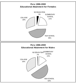
These average figures from 1986-2000 show an important evolution. The percentage of working females with a college or high school degree increased from 68% to 81%, while for their male peers the increase was from 78% to 84%.
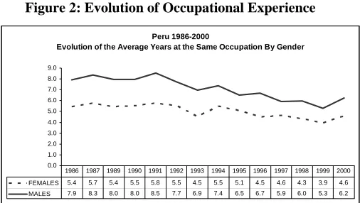
[image:4.595.171.423.344.622.2]The greatest gender difference is found in the working people's occupational experience, measured as years working in the same occupation (illustrated in Figure 2). For the period in consideration, on average, males have between 1.4 and 2.7 more years of occupational experience than females – between a 30% and a 50% difference. It should be noted, however, that these gender differences in average years of occupational experience have decreased substantially from 1986-2000.
Figure 1: Educational Attainment by Gender
Peru 1986-2000
Educational Attainment for Females
NO EDUCATION
3% ELEMENTARY SCHOOL
21% COLLEGE
30%
HGH SCHOOL 46%
Peru 1986-2000 Educational Attainment for M ales
NO EDUCATION 1%
ELEMENTARY SCHOOL
15%
HGH SCHOOL 50% COLLEGE
Figure 2: Evolution of Occupational Experience
Peru 1986-2000
Evolution of the Average Years at the Same Occupation By Gender
0.0 1.0 2.0 3.0 4.0 5.0 6.0 7.0 8.0 9.0
FEMALES 5.4 5.7 5.4 5.5 5.8 5.5 4.5 5.5 5.1 4.5 4.6 4.3 3.9 4.6
MALES 7.9 8.3 8.0 8.0 8.5 7.7 6.9 7.4 6.5 6.7 5.9 6.0 5.3 6.2
1986 1987 1989 1990 1991 1992 1993 1994 1995 1996 1997 1998 1999 2000
Regarding the differences in the supports highlighted by the matching methodology, I find that 30% of working females exhibit combinations of age, education, migratory condition9 and marital status that cannot be matched by any male in the sample. Likewise, 23% of working males report combinations of the same individual characteristics (age, education, migratory condition and marital status) that cannot be matched by any female in the sample. This 23% of working males report wages that are considerably higher than those reported by the rest of the working males.
As noted, there are gender differences in some observable characteristics that the labor market rewards. However, these gender differences have been narrowing during the period in consideration. The next section will explore the relationship between the characteristics previously shown and the hourly wage, partially explaining the gender wage gap and its evolution.
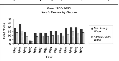
Wages evolved considerably during the period of analysis. After the rise in real wages that started in 1985 and continued until 1987, a significant fall in real wages at a time of hyperinflation followed. Real wages reached their minimum level in 1990 and subsequently improved. During the nineties, real wages increased steadily until the late years of the decade, when once again they began to decline. Figure 3 shows this evolution of the hourly wage for males and females. The hourly wages are measured in constant 1994 Peruvian Soles.
Figure 3: Hourly Wages by Gender (in 1994 Soles)
Peru 1986-2000 Hourly Wages by Gender
0 5 10 15 20 25 30
19 86
19 87
19 89
19 90
19 91
19 92
19 93
19 94
19 95
19 96
19 97
19 98
19 99
20 00
Year
1
994 S
o
le
s
Male Hourly Wage
Female Hourly Wage
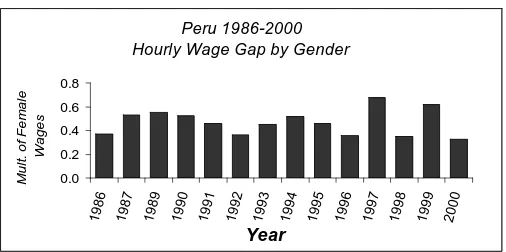
This graph shows the absolute values (in constant 1994 Soles) of the gender wage gap (represented by the difference between a pair of adjacent columns). Figure 4 shows the gap in relative terms (average hourly wage gap as multiples of average hourly female earnings).10 It can be found that the gender wage gap in hourly wages vacillated around an average value of 0.45 (that is, males earned an average of 45% more per hour than females). However, there are significant fluctuations around that average measure.
The measure of the gap that is reported in this section (multiples of average hourly wages for females) is crude data since it considers all males and females regardless of their differences in observable characteristics, and regardless of whether it is possible to compare them or not. It is necessary to make the appropriate adjustments to that gap in order to obtain a measure of unexplained differences in average earnings for comparable samples of males and females. That is the purpose of the next sub-section, but before starting that exercise let us explore how these gender differences in average hourly wages vary according to individual characteristics.
Regarding age, once the population has reached 30, the gender wage gap tends to increase and for people close to retirement, the age gap reaches 128%.11
10Note that the variable in which the gender gap is measured in this paper is hourly wage instead of using the
logarithm of the hourly wage as is commonplace in the literature. With matching, such transformation is no longer required.
11It is important to note that this basic computation of average wage gaps for different age groups mixes age
According to educational attainment, the gender wage gap exhibits non-monotonic behavior. There is a larger gap for people with only an elementary education and people with college degrees. The gap diminishes for the uneducated and high school populations.
Figure 4: Hourly Wage Gap by Gender (in 1994 Soles)
Peru 1986-2000 Hourly Wage Gap by Gender
0.0 0.2 0.4 0.6 0.8
19 86
19 87
19 89
19 90
19 91
19 92
19 93
19 94
19 95
19 96
19 97
19 98
19 99
20 00
Year
M
u
lt
. o
f F
e
m
a
le
Wa
g
e
s
Figure 5: Hourly Wages and Gender Wage Gap for Different Age Groups
PERU 1986-2000
HOURLY WAGES ACCORDING TO GENDER AND AGE
(In 1994 Soles)
Less Than 19 Years
20 to 29 30 to 44 45 to 60 60 or
more
FEMALES 5.58 10.03 12.97 12.45 10.17
MALES 7.62 11.99 17.11 20.32 23.16
[image:7.595.172.425.256.382.2]GAP 37% 20% 32% 63% 128%
Figure 6: Hourly Wages and Gender Wage Gap by Educational Attainment
PERU 1986-2000
HOURLY WAGES ACCORDING TO GENDER AND EDUCATION (In 1994 Soles)
NO EDUCATION
ELEMENTARY SCHOOL
HGH SCHOOL COLLEGE
FEMALES 6.52 6.83 9.56 16.32
MALES 7.79 10.22 11.86 23.81
The previous tables reveal substantial differences in the distribution of wages and the gender wage gap according to individual characteristics, each analyzed independently. Next, I will analyze the joint effects of these differences in characteristics on wages, using the matching and decomposition approach.
3. Explained and Unexplained Components of the Gender Wage Gap
3.1 Wage Gap Decomposition. The Matching Approach
Recalling from Ñopo (2004), the wage gap,
∆
,
can be expressed as:[
Y
|
M
] [
E
Y
|
F
]
M X 0 F.
E
−
=
∆
+
∆
+
∆
+
∆
=
∆
The average wage difference between males and females can be broken into four components. Three of them can be attributed to gender differences in observable individual characteristics
(
)
F X
M ∆ ∆
∆ , and and the fourth component to the existence of both non-observable gender differences in characteristics that determine wages and gender discrimination in pay
( )
:0
∆
X
∆
is explained by the fact that males and females tend to have individual characteristics that are distributed differently over their common support. For instance, in the Peruvian data sets it is possible to find both males and females with Masters or Ph.D. degrees, but the proportion of females under that category is substantially smaller than the proportion of males.X
∆ accounts for the expected decrease in male wages when their individual characteristics follow the distribution of female characteristics.
F
∆ is explained by the fact that there are some combinations of female characteristics for which there are no comparable males. For instance, in the Peruvian data sets there are some married females, migrants, with zero or only a few years of schooling and some years of occupational experience, but it is impossible to find males with those combinations of characteristics.
F
∆ measures the expected increase in wages that the average female will experience assuming all females achieve characteristics that are comparable to those of males.
M
find females with such characteristics.
M
∆ measures the expected increase in wages that the average female wages would have, if females achieve those individual characteristics of males that remain unreached by females.
0
∆ represents that which cannot be explained by these differences in observable characteristics. This can be explained as a combination of discrimination in pay and the existence of gender differences in unobservable characteristics that are related to productivity.
For additional details regarding the decomposition's derivation, see Sub-section 3.1 in Ñopo (2004).
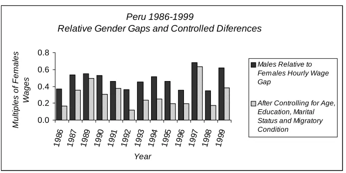
Figure 7 represents the evolution of the crude gender wage gap12 accompanied by the wage gap when controlling for age, education, marital status and migratory condition when matching. The chart is reporting the evolution of the crude data and controlled data (
∆
and0
[image:9.595.125.472.392.566.2]∆ respectively).13
Figure 7: Gender Wage Gap After Controlling for Observable Characteristics
Peru 1986-1999
Relative Gender Gaps and Controlled Diferences
0.0 0.2 0.4 0.6 0.8
19 86
19 87
19 89
19 90
19 91
19 92
19 93
19 94
19 95
19 96
19 97
19 98
19 99
Year
M
u
lt
ip
le
s o
f
F
e
m
a
le
s
W
ages
Males Relative to Females Hourly Wage Gap
After Controlling for Age, Education, Marital Status and Migratory Condition
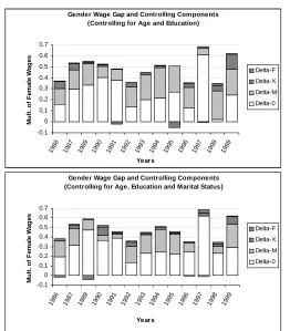
Figure 8 represents the wage gaps measured in relative terms (as multiples of female wages) and the decompositions in terms of the four components introduced above. The total height of each bar is proportional to the wage gap
12
The measure of wage gap that I am using is
−
1
F M
y
y .
13For this and the next decompositions, I omit the one that corresponds to the year 2000 due to a problem of
in the respective year. The height of each component is proportional to the value of the respective component, such that whenever a component has a negative value, it is illustrated below the zero line. The first set of decompositions reported below has been calculated using different combinations of explanatory variables such as age (measured in years), education (measured in years of schooling), marital status (a dichotomous variable that takes the value 0 for singles and 1 for married individuals) and migratory condition (a dichotomous variable that distinguishes individuals who were born in Lima from those who were born elsewhere).
Figure 8: Wage Gap Decompositions for Different Sets of Controls (1)
Gender Wage Gap and Controlling Com ponents (Controlling for Age and Education)
-0.1 0 0.1 0.2 0.3 0.4 0.5 0.6 0.7
198 6
198 7
198 9
199 0
199 1
199 2
199 3
199 4
199 5
199 6
199 7
199 8
199 9 Years M u lt . o f F e m a le W a g e s Delta-F Delta-X Delta-M Delta-0
Gender Wage Gap and Controlling Com ponents (Controlling for Age, Education and Marital Status)
Figure 9: Wage Gap Decompositions for Different Sets of Controls (2)
Gender Wage Gap and Controlling Com ponents (Controlling for Age, Education and Migratory Condition)
-0.1 0 0.1 0.2 0.3 0.4 0.5 0.6 0.7 19 86 19 87 19 89 19 90 19 91 19 92 19 93 19 94 19 95 19 96 19 97 19 98 19 99 Years M u lt
. of Fe
m a le W a ge s Delta-F Delta-X Delta-M Delta-0
Gender Wage Gap and Controlling Com ponents (Controlling for Age, Educ., Marit. Status and Mig. Cond.)
-0.1 0 0.1 0.2 0.3 0.4 0.5 0.6 0.7
198 6
198 7
198 9
199 0
199 1
199 2
199 3
199 4
199 5
199 6
199 7
199 8
199 9 Years M u lt . o f F e m a le W a g e s Delta-F Delta-X Delta-M Delta-0
While the gender wage gap without controlling for characteristics, has an average value of 45% during the period of analysis, the controlled gap,
0,
teeters around 28%.
,
∆
∆ 14Thus, the mixture between gender differences not considered in the analysis (which may comprise observable and unobservable differences) and discrimination account for a differential of 28% in hourly wages between males and females. These figures correspond to the particular set of variables specified above. This set does not include variables that are typically considered as being determined endogenously in the labor market. Combinations of these variables are considered for the following
14As will be shown later in the paper, a 99% confidence interval for the average unexplained gender
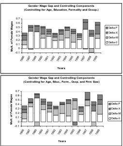
decompositions. For the decompositions in Figure 10, I consider different combinations of age, education, occupational experience (measured in years), informality (a dichotomous variable that distinguishes individuals with formal jobs from individuals with informal jobs15), occupation (that comprises seven occupational categories) and firm size (with five categories).
Figure 10: Wage Gap Decompositions for Different Sets of Controls (3)
Gender Wage Gap and Controlling Com ponents (Controlling for Age, Education and Form ality)
-0.1 0 0.1 0.2 0.3 0.4 0.5 0.6 0.7 19 86 19 87 19 89 19 90 19 91 19 92 19 93 19 94 19 95 19 96 19 97 19 98 19 99 Years Mu lt . o f F e m a le W a g e s Delta-F Delta-X Delta-M Delta-0
Gender Wage Gap and Controlling Com ponents (Controlling for Age, Education, Form . and Firm Size)
-0.1 0 0.1 0.2 0.3 0.4 0.5 0.6 0.7
198 6
198 7
198 9
199 0
199 1
199 2
199 3
199 4
199 5
199 6
199 7
199 8
199 9 Years M u lt . o f F e m a le W a g e s Delta-F Delta-X Delta-M Delta-0
15A job is considered formal if it satisfies at least one of the following requirements: being in the Public
Figure 11: Wage Gap Decompositions for Different Sets of Controls (4)
Gender Wage Gap and Controlling Com ponents (Controlling for Age, Education, Form ality and Occup.)
-0.1 0 0.1 0.2 0.3 0.4 0.5 0.6 0.7
198 6
198 7
198 9
199 0
199 1
199 2
199 3
199 4
199 5
199 6
199 7
199 8
199 9 Years M u lt . of Fe m a le W a ge s Delta-F Delta-X Delta-M Delta-0
Gender Wage Gap and Controlling Com ponents (Controlling for Age, Educ., Form ., Occp. and Firm Size)
-0.1 0 0.1 0.2 0.3 0.4 0.5 0.6 0.7
198 6
198 7
198 9
199 0
199 1
199 2
199 3
199 4
199 5
199 6
199 7
199 8
199 9 Years Mu lt . o f F e m a le W a g e s Delta-F Delta-X Delta-M Delta-0
The average unexplained gender wag gap
( )
0
∆
after controlling for these endogenous characteristics is around 25%, slightly below the average when they are not considered.16 Interestingly, for almost every combination of characteristics I considered in the previous exercises, the controlled gender wage gap shows two peaks: one at the end of the 1980's, during the period of hyperinflation, and another in the middle of the 1990's during the recession that followed the stabilization of 1990-1994. Also, the lower values for the gap are found around 1986 and 1993 – years that register significant Peruvian GDP growth.16A detailed spreadsheet with the results for all the decompositions showed here, as well as some other
In analyzing the role that the four delta components play in the decomposition, it is discovered that the components
0
∆
andM
∆ explain more than 80% of the wage gap during all years for almost all possible combinations of characteristics. As mentioned earlier in this section, both components of the gap may be regarded as noisy discrimination measures or unexplained differences. The first of them is determined in the labor market and the second determined outside of the labor market (in the acquisition of such valuable characteristics). While the former is linked to differences in pay, the latter is presumably linked to differences in access to particular combinations of characteristics that are rewarded in the labor market.
Next, I analyze the distribution of the unexplained gender differences in pay that can be obtained from the matching approach. I will compare the distribution of wages for females to the counterfactual distribution of wages for males when they are resampled in order to mimic the distribution of females' characteristics.
3.2 Differences in Hourly Wages Between Matched Samples17
A common critique of the Blinder-Oaxaca decomposition is that it is informative only in reference to the average gaps and not the distribution of these gaps. An alternative has been to use quantile regressions instead of O.L.S., decomposing gender wage gaps at different quantiles of the distribution of the error term of the earnings equations. This approach suffers from the same problem of the gender differences in the supports that the matching methodology addresses.
This sub-section is devoted to the analysis of the distribution of wages for males and females. The object of analysis will be the cumulative distribution functions of hourly wages for the original and matched samples of females and males.
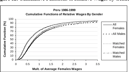
By plotting the cumulative functions, it is possible to verify that not only are average wages for males greater than average wages for females, but also the random variable wages for females is stochastically dominated by the random variable wages for males. The result is the same if the comparison is made between the resampled (by matching) versions of the same random variables. Even after controlling for age, schooling, marital status and migratory condition, there are gender differences in pay that favor males, as
seen in Figure 12. To better visualize these differences in the cumulative functions, Figure 13 shows an extract of Figure 12.
Figure 12: Cumulative Functions of Relative Wages by Gender
Peru 1986-1999
Cumulative Functions of Relative Wages By Gender
0 10 20 30 40 50 60 70 80 90 100
0 0.5 1 1.5 2 2.5 3 3.5
Mult. of Average Females Wages
C
u
m
u
la
ti
v
e
Func
ti
on (
%
)
All Females All Males
[image:15.595.166.428.391.528.2]Matched Females Matched Males
Figure 13: Cumulative Functions of Relative Wages by Gender (Extract)
Peru 1986-1999
Cumulative Functions of Relative Wages By Gender
40 50 60 70 80 90 100
0.5 1 1.5 2 2.5 3 3.5
Mult. of Average Females Wages
C
u
m
u
la
ti
v
e
Func
ti
on (
%
)
All Females All Males
Matched Females Matched Males
component of the gap is relatively small compared to the other components). For males, the situation is different. The cumulative distribution of hourly wages for all males differs from the distribution of only matched males (with the appropriate re-weighting that is required to mimic the empirical distribution of individual characteristics of females), especially at the upper extreme of the distribution.
[image:16.595.172.426.451.593.2]The previous plot inspires a quantile analysis since at any height (percentile) of the previous two graphs (the horizontal distance between the two cumulative functions obtained after matching) measures the unexplained gender wage gap at that respective percentile. Figure 14 shows these measures. The plot shows that for the first ninety percentiles of the distribution of hourly wages for males and females there are no major differences in hourly wages. The gap is slightly below 0.2 times the average wage for females. The highest differences are found in the top 10% of the distributions of hourly wages. At the 99th percentile the gap attains a maximum where the average wage of males is 2.2 times the average wage of females. The plot shows evidence that the gender differences in pay in the bottom percentiles of the distribution do not contribute considerably to the aggregate measure of gender differences in pay. The average gender wage gap in Peru is driven by gender differences in pay at the top percentiles of the wage distributions.
Figure 14: Absolute Gender Wage Gap by Percentiles
Peru 1986-1999
Absolute Gender Wage Gap (After Matching) by Percentiles
0 0.4 0.8 1.2 1.6 2 2.4
0 10 20 30 40 50 60 70 80 90 100 Percentile of Wage Distribution
M
u
lt
ip
le
s
o
f
A
v
e
ra
g
e
Wag
e
s
fo
r F
e
m
a
le
s
premium of 12% of average female wages compared to the 10th percentile female (approximately 1.40 1994 Peruvian Soles). However, this represents a difference of 60%. When the same comparison is made at the lowest percentile the differences are even more dramatic. The hourly wage gap in absolute terms is approximately 0.70 1994 Peruvian Soles, but that figure represents a difference of 94%. The poorest male earns almost twice as much as the poorest female. These percentage differences in hourly wages by percentiles of the wage distributions are shown in Figure 15.
Figure 15: Relative Gender Wage Gap by Percentiles
Peru 1986-1999
Relative Gender Wage Gap (After Matching) by Percentiles
0% 20% 40% 60% 80% 100%
0 10 20 30 40 50 60 70 80 90 100 Percentile of Wage Distribution
P
e
rcen
ta
g
e
The relative gender wage gap by wage percentiles shows a slight U-shape in which the minimum gap, 18%, is found among those individuals whose wages are between the 8th and 9th deciles. The maximum is found among the poor.
3.3 Confidence Intervals for Average Unexplained Gender Differences in Pay
The analysis of the distribution of unexplained gender differences in pay can also be done through the computation of confidence intervals. The
method
−
Figure 16: Standard Errors for the Average Unexplained Gender Wage Gap
Mean Std. Error
All 0.2803 0.0189
Marital Status
Single 0.2751 0.0242
Maried 0.2862 0.0289
Migratory Condition
Born in Lima 0.3067 0.0300
Born out of Lima 0.2840 0.0269
Peru 1986-1999
Unexplained Gender Wage Gap By Selected Characteristics (After Controlling for Age, Education, Marital Status and Migratory Condition)
The average unexplained gender wage gap of 28.03% has a standard error of 1.89%. This translates into a 99% confidence interval for the average unexplained differences in pay that ranges from 24.92% to 31.13% of average female wages. Concerning migratory condition, there is evidence that the unexplained differences in pay are smaller among migrants than among those who were born in Lima. Regarding marital status, although there is no clear evidence that the average unexplained gender differences in pay between married and single individuals are substantially different, there is more evidence of dispersion of such unexplained differences among the married than among the singles. The higher dispersion of unexplained wages could be explained in terms of other variables that are considered endogenous to a model of wage determination in the labor market, such as occupational experience, tenure, hours worked per week and occupation. It is more likely to observe higher dispersion in these variables among the married than among the single.
roughly correspond to the deciles of the age distribution of the employed labor force in Lima, Peru.
Figure 17: Confidence Intervals for the Unexplained Gender Wage Gap (1)
Unexplained Gender Wage Gap By Age
(After Controlling for Age, Education, Marital Status and Migratory Condition) Single Individuals -0.4 0 0.4 0.8 1.2
<20 >=20 &
<23 >=23 & <27 >=27 & <30 >=30 & <33 >=33 & <37 >=37 & <42 >=42 & <47 >=47 & <54 >=54 Age M u lt ip le o f F e m a le W a g e s
Figure 18: Confidence Intervals for the Unexplained Gender Wage Gap (2)
Unexplained Gender Wage Gap By Age
(After Controlling for Age, Education, Marital Status and Migratory Condition) Married Individuals -0.4 0 0.4 0.8 1.2
<20 >=20 &
<23 >=23 & <27 >=27 & <30 >=30 & <33 >=33 & <37 >=37 & <42 >=42 & <47 >=47 & <54 >=54 Age M u lt ip le o f F e m a le W a g e s
[image:19.595.173.422.446.621.2]some evidence of an increasing evolution of these unexplained differences over the life cycle, but that increase is not significant from decile to decile. However, while the unexplained differences in pay are positive for married individuals above the median age (33 years), these differences are not different than zero for those who are younger than the median. The dispersion of such unexplained differences increase over the singles' life cycles.
In analyzing unexplained gender differences in pay according to years of schooling there are more issues (Figures 19 and 20). These unexplained differences are positive and almost constant for individuals with less than a high school diploma (less than 11 years of schooling) – especially for single individuals. Also, for singles that attended between 4 and 11 years of schooling (which corresponds to 30% of the total employed labor force), there is smaller dispersion in the unexplained gender wage gap. Among high school graduates (those who completed 11 years of schooling and represent 35% of the total employed labor force), there is less evidence for unexplained gender differences in pay – especially among the married.
Figure 19: Confidence Intervals for the Unexplained Gender Wage Gap (3)
Unexplained Gender Wage Gap By Years of Schooling (After Controlling for Age, Education, Marital Status and Migratory Condition)
Single Individuals
-0.6 0 0.6 1.2 1.8 2.4 3
0 1 2 3 4 5 6 7 8 9 10 11 12 13 14 15 16 17
Years of Schooling
M
u
lt
ip
le
o
f F
e
m
a
le
W
a
g
e
s
Figure 20: Confidence Intervals for the Unexplained Gender Wage Gap (4)
Unexplained Gender Wage Gap By Years of Schooling (After Controlling for Age, Education, Marital Status and Migratory Condition)
Married Individuals
-0.6 0 0.6 1.2 1.8 2.4 3
0 1 2 3 4 5 6 7 8 9 10 11 12 13 14 15 16 17
Years of Schooling
M
u
lt
ip
le
o
f F
e
m
a
le
W
a
g
e
[image:21.595.171.425.413.587.2]4. Has there been a Decrease in the Gender Wage Gap?
According to the measure reported for unexplained gender differences in pay in the previous section, there is no evidence of a monotonic decrease of such differences. The hourly gender wage gap reached its lowest levels during 1992 and 1999 while it attained peaks during 1989 and 1997, evolving in a way that seems correlated with the cycle of the Peruvian economy. That measure of gender differences does not take into consideration either labor market participation effects or unemployment rates. There are changes in female participation and unemployment rates over the period of analysis, especially after the labor market reforms undertaken during the first half of the nineties.
While participation rates for males do not change dramatically over the period of analysis, participation rates among females slightly decreased at the beginning of the nineties and then increased towards the latter half of the decade – a decrease in the differences in participation rates from 28% to 21% over the entire period. Also, gender differences in unemployment rates decreased. While the male unemployment rate increased from 4% to 7% during the fifteen-year span, the female unemployment rate evolved with substantial ups and downs, reporting a slight increase from 8% to 9% during the whole period. The peaks reported in this evolution of female unemployment rates coincide with peaks in unexplained gender differences in hourly wages (one at the end of the eighties, another during the stabilization period from 1992-1994 and a third in 1997). These changes are correlated with the cycle of the economy. Higher gender differences in unemployment rates are linked to higher unexplained gender differences in pay.
unexplained differences that, as usual, can be regarded as a sign of the existence of both discrimination and unobservable characteristics determining participation (unemployment).
Figures 21 and 22 report the evolution of gender differences in participation and unemployment rates together with the controlled (by matching) versions of such rates for males, considering age, education, marital status and migratory condition as matching variables applied to the whole population. The results suggest that gender differences in age, education, marital status and migratory condition do not explain gender differences in participation or unemployment rates. If anything, the controlled unemployment rates for males are slightly smaller than the crude unemployment rates. There are other determinants of such differences, and discrimination may be one of those, but it also may be choice – it is impossible to decipher from the data.
Figure 21: Participation Rates by Gender
Urban Peru 1986-2000 Evolution of Participation Rates by Gender
40% 45% 50% 55% 60% 65% 70% 75% 80% 85%
198 6
198 7
198 9
1 99 0
199 1
199 2
199 3
199 4
199 5
199 6
199 7
199 8
199 9 2 00 0 Year P e rc e n tage Fermales Males
[image:23.595.169.427.369.601.2]Males after controlling for age, education, marital status and migratory condition
Figure 22: Unemployment Rates by Gender
Urban Peru 1986-2000 Evolution of Unemployment Rates by Gender
0% 2% 4% 6% 8% 10% 12% 14%
198 6
198 7
198 9
199 0
199 1
199 2
199 3
199 4
199 5
199 6
199 7
199 8
199 9
200 0 Year P e rc e n tage Fermales Males
Males after controlling for age, education, marital status and migratory condition
females worked 41 hours. This represents an approximate 16% difference in the average number of hours worked by men versus that of women. These differences have decreased over the period 1986-2000. While males worked 21% more hours than females in 1986, they worked for 13% more hours than females during 2000.
[image:24.595.167.427.352.454.2]Figure 23 shows the evolution of gender differences in the Peruvian labor market using a measure of earnings that incorporates participation at the intensive and extensive margins. For this purpose, the measure to analyze is the Fraction of Total Labor Income Generated by Males, computed individually. If there were no gender differences in participation, employment and pay in the labor markets, this measure would be valued at 50%. If only males generate labor income, this measure would be valued at 100%.
Figure 23: Fraction of Total Labor Income Generated by Males
Urban Peru 1986-2000
Fraction of Total Labor Income Generated by Males
50% 60% 70% 80%
1986 1987 1989 1990 1991 1992 1993 1994 1995 1996 1997 1998 1999 2000
Year
P
e
rcent
a
ge
Figure 24: Fraction of Total Labor Income Generated by Males (by Age Groups)
Urban Peru 1986-2000
Fraction of Total Labor Income Generated by Males for Different Age Groups
50% 60% 70% 80%
1986 1987 1989 1990 1991 1992 1993 1994 1995 1996 1997 1998 1999 2000
Year
P
e
rcent
a
g
e
Older People (33 years old and more)
Younger People (less than 33 years old)
As mentioned, this measure is crude in the sense that it does not take into account gender differences in the individual characteristics that determine participation, employment and wages. Again, the generation of a counterfactual is required in order to answer the question: What fraction of total labor income males would generate if their individual characteristics were distributed according to the empirical distribution of the individual characteristics of females?
The same matching algorithm previously applied to understand the differences in participation and unemployment rates can be applied here. Now, the measure that matters for the purpose of this new exercise is the total labor income generated by females and males in the matched sample. The variables considered for this matching exercise – age, education, marital status and migratory condition – are exogenous to the labor market.
Figure 25: Fraction of Total Labor Income Generated by Males (After Matching)
Peru 1986-2000
Fraction of Total Labor Income Generated by Males
60% 65% 70% 75% 80%
1986 1987 1989 1990 1991 1992 1993 1994 1995 1996 1997 1998 1999 2000
Year
Pe
rc
e
n
ta
g
e
Fraction of Total Labor Income
Fraction Af ter Controlling f or Age and Education Fraction Af ter Controlling f or Age, Education, Marital Status and Migratory Condition
[image:25.595.165.433.482.584.2]such differences in generation of labor income (among which we can consider discrimination). Moreover, for the last years of our analysis the controlled fraction exceeds the crude fraction. This is explained by an increase in years of education for females that is not accompanied by a corresponding increase in labor income. Females are acquiring more education but they are getting neither more jobs nor higher pay.
5. Conclusions
By using a matching comparisons approach, this paper raises new findings about gender differences in the Peruvian labor markets. Approximately one out of four workers in Peru exhibit individual characteristics that are not comparable to workers of the opposite sex. This form of gender differentiation in characteristics that the labor market depicts has a clear impact on the wage gap. Males who report observable characteristics that are unmatchable by females exhibit higher wages than the average worker, while females who report unmatchable observable characteristics exhibit lower wages than the average worker.
The most interesting finding is the wage gap that subsists after matching males and females with the same observable individual characteristics (age, education, marital status and migratory condition). Among comparable males and females the wage gap is approximately 28% of the female wages. Also, the matching approach allows us to explore the distribution of such average measure. The gender wage gap is not evenly distributed among the working population. It is in the lowest extreme of the distribution of wages where the gender wage gap is the biggest, attaining about 100%.
References
Blau, F. and Ferber, M. (1992), “The Economics of Women, Men and Work.” 2nd Ed. Englewood Cliffs, NJ: Prentice-Hall.
Blinder, A. (1973), “Wage Discrimination: Reduced Form and Structural Estimates.” The Journal of Human Resources, VII, 4, pp. 436-55.
Ñopo, H. (2004), Matching as a Tool to Decompose Wage Gaps. (January 2004). IZA Discussion Paper No. 981.
Oaxaca, R. (1973), Male-Female Wage Differentials in Urban Labor Market. International Economic Review, Vol.14, No.3, 693-709.
Saavedra, J. (2000), “La Flexibilización del Mercado Laboral.” In La Reforma
Incompleta: Rescatando los Noventa. Abusada, Roberto Ed. Universidad del
Pacífico, Lima, 379-428
Saavedra, J. and Torero, M. (2000), “Labor Market Reforms and Their Impact on Formal Labor Demand and Job Market Turnover: The Case of Peru.” Inter-American Development Bank, Research Department, Research Network
Working Paper #394. Washington D.C.
THE GENDER WAGE GAP IN PERU 1986-2000:
EVIDENCE FROM A MATCHING COMPARISONS APPROACH
HUGO ÑOPO
SUMMARY
JEL Classification: C14, D31, J16, O54.
Applying the methodology developed in Ñopo(2004), I analyze the evolution of the gender wage gap in Peru from 1986 to 2000. The advantage of such methodology is two-fold. First, it recognizes that the supports of observable characteristics distributions differ substantially. Second, it provides deeper insights regarding the distribution of the unexplained gender differences in earnings.
For the period under analysis, males earn on average 45% more than females. This wage gap is composed of three additive elements: 11% differences in supports, 6% differences in distributions of individual characteristics and 28% unexplainable differences. About half of these unexplainable differences occur in the highest quintile of the wage distribution.