Time series modeling and synchronization using neural networks

Time Series Modeling and Synchronization

using Neural Networks

A. S. Cofi˜no and J.M. Guti´errez

Dept. of Applied Mathematics, University of Cantabria, E-39005, Santander, Spain

[email protected], [email protected], WWW home page: http://ccaix3.unican.es/~gutierjm

Abstract

In the last few years, neural networks have found interesting applications in the field of time series modeling and forecasting. Some recent results show the ability of these models to approximate the dynamical behavior of nonlinear chaotic systems, leading to similar dimensions and Lyapunov exponents. In this paper we analyze further the dynamical properties of neural networks when comparted with chaotic systems. In particular, we show that the possibility of synchronizing chaotic systems gives a natural criterion for determining similar dynamical behavior between these systems and neural approximate models. In particular we show that a neural model obtained from an experimental scalar laser-intensity time series can be synchronized to the time series, indicating that it captures the dynamical behavior of the system underlying the data.

Keywords

1

Introduction

Time series analysis is an important discipline which deals with the modeling, control and forecast of real-world systems from a set of measured observations. Several methods for obtaining linear approximate models have been developed for this purpose, including the well-known ARMA models (see [1] for a introduction to linear time series analysis). The main goal of these methods is, first, fitting an appropriate model to the data and, then, using the obtained model for predicting the future, or for controlling the system’s state. These ideas have been applied in a great variety of domains, going from Economics to Physics or from Engineering to Social Sciences, resulting in the identification of linear deterministic models underlying many time series associated with interesting problems.

However, in the last two decades a great deal of attention has been focused in nonlin-ear systems, which can exhibit a complex seemingly stochastic behavior known as deter-ministic chaos. This interest was mainly motivated by the discovering of chaos in simple low-dimensional nonlinear models, and in a great variety of experimental time series (stock markets [2], electronic circuits [3], biology [4], etc.). Although at first sight a chaotic system may seem unpredictable and unmanageable, its deterministic low-dimensional nature allows distinguishing it from noise and makes feasible reconstructing its functional structure from a time series using appropriate nonlinear techniques.

In recent years new approaches for nonlinear time series modeling have emerged (local and global prediction [5], neural networks [6], delay reconstruction space [7], wavelets [8], functional networks [9], etc.), providing more powerful methods and giving new insight into the dynamics of these systems (see [10] and references therein for an updated survey of this topic). Among these techniques, artificial Neural Networks (NNs) have been successfully applied in many practical situations [11, 12, 13]. Moreover, it has been shown that under some circumstances a neural approximate model resemble the original system, in the sense that both the original and neural models can exhibit similar unstable periodic orbits [14], or even similar Lyapunov exponents or fractal dimension [15] (see [16] for more details about these topics).

However, there is no general quantitative criterion for deciding whether a reconstructed model can be considered a dynamical approximation of the original system. This problem is specially important when there is no knowledge about the functional form of the system and the only information available is a scalar time series sampled from the system (note that this is always the situation in many experimental problems). In most cases, the residual error between the predicted and real values is used as a quantitative criterion for this purpose. However, in some cases low-error models can be overfitted to the data, leading to a wrong reconstruction of the system dynamics.

Syn-chronization was also found to be robust to small perturbations on the system parameters, so slightly different systems could also be synchronized. Therefore, the robustness of chaotic synchronization can be used as a natural criterion for determining similar dynamical be-havior among different systems. In particular, this criterion can be applied to check the performance of different neural models obtained from a time series when compared with the underlying dynamical system. To illustrate the ideas presented in the paper, we shall analyze both computer-generated times series obtained by simulating simple deterministic dynamical systems (such as the Lorenz model), and an experimental scalar time series obtained from a

N H3 infrared laser.

This paper is structured as follows. In Section 2 we present some basic results about NNs and their application to time series modeling. In Section 3 we describe chaos synchroniza-tion and show the possibility of synchronizing neural models with chaotic systems; we also describe the application for characterizing similar dynamical behaviors. Finally, Section 4 describes a real-world application of the technique using an experimental scalar time series.

2

Modeling Chaotic Systems with Neural Networks

It is now generally recognized that seemingly random time series may be the result of some stochastic process, but they may also be produced by some simple nonlinear system. In either case, a long-term prediction is possible only in probabilistic terms. However, in the short term, low-dimensional chaotic systems can be predicted by fitting an appropriate functional model to the available data for reconstructing its underlying functional structure.

Suppose we are given a time series un, obtained from a dynamical system given by a

flow ˙u(t) = F(u(t)), sampled at equally spaced intervals tn = n τ, n = 0,1,2, . . .. We are

interested in approximating the functional model which characteries the short-term evolution of the time series, un+p =f(un), where f is given in terms of F, the sampling timeτ, and

the prediction horizon p.

To this aim we shall consider simple feed-forward NNs with sigmoidal σ(x) = 1 1+e−x and linear activation functions for hidden and output layers, respectively. This type of network has shown to be an universal approximator for continuous (one hidden layer) or arbitrary (more than one hidden layer) functions [18]. The training process is carried out by considering input–output couples of the form (un,un+p), where p is the prediction horizon.

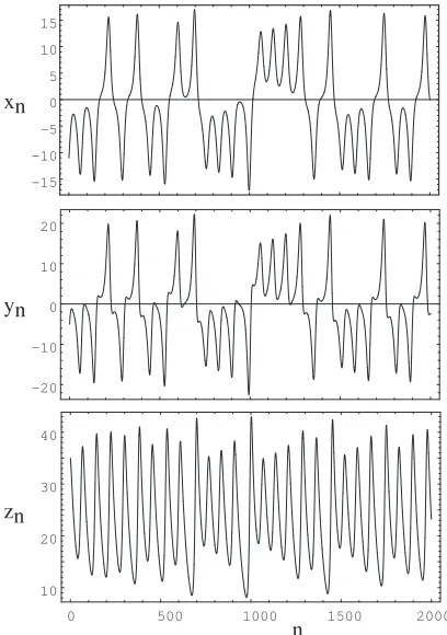
To illustrate the concepts we shall use the well known Lorenz model, given by the set of differential equations [19]:

( ˙x,y,˙ z˙) = (σ(y−x),−x z+r x−y, x y−b z) (1)

xn

n

-15 -10 -5 0 5 10 15

-20 -10 0 10 20

0 500 1000 1500 2000 10

20 30 40

yn

zn

set was divided in two parts; the first one was used for training whereas the second one was reserved for testing the models.

Figure 1: Time series of the Lorenz system obtained with a sample timeτ = 10−2.

Since we are dealing with a continuous system, we have considered different NNs with three input neurons (xn, yn, zn), three output neurons (xn+1, yn+1, zn+1), and a single hidden layer containing from one to twenty neurons (this type of architecture is usually referred to as a 3 :a: 3 feedforward network, wherea is the number of hidden neurons). For each of these network structures, ten experiments were performed with different initial network weighs, using the Levenberg-Marquardt method as training algorithm; the best solution in each case was considered as the representative neural approximate model. For instance, Figure 2(a) shows the errors obtained for predicting x variable with the best six hidden neurons NN obtained:

ˆ

xn+1 = −3768.18−

0.34

1 +e9.31+0.53xn−0.68yn−0.21zn +

0.92

1 +e7.64−0.121xn−0.149yn−0.13zn −

2.75

1 +e6.19+0.15xn+0.0451yn−0.09zn −

2.04

1 +e1.13+0.06xn+0.0119yn−0.06zn + (2)

7164.31

1 +e−0.12+0.00021xn−0.0002yn+0.000021zn −

63.52

1 +e−0.24+0.08xn−0.016yn+0.0049zn

200 400 600 800 1000 -0.015

0 0.015

-0.015 0 0.015

200 400 600 800 1000

-0.1 0 0.1

-0.1 0 0.1

(a)

(b)

x

n

-x

n

n

x

n

-x

n

Figure 2: Residuals xn−xˆn for two neural models with (a) six and (b) fifteen hidden units.

The neural nets are trained with the first 500 points and a cross validation is performed with the last 500 points. No overfitting can be appreciated in the models.

which gives a Root Mean Square Error (RMSE) 0.133 for the training process, that is less than 0.5% the range of the corresponding variable, and 0.149 for the test data. These results clearly indicate a good performance of the neural model, since no overfitting is detected.

However, although the above analysis indicates a good accuracy in one-step ahead pre-diction using a six neuron NN, it is not clear that the obtained neural model can reproduce the dynamics of the Lorenz system. Figure 3 illustrates this fact by showing the evolution of two different NNs; in the first case, the neural system converges to a periodic trajectory (Fig. 3(a)), whereas in the second case it converges to a fixed point (Fig. 3(b)), neither of them resembling the chaotic behavior of the lorenz model. As we have seen in this example, an interesting result obtained when training NNs with a low number of parameters is that the resulting orbits may not behave as the original chaotic system, but resemble some unstable periodic orbits embedded in the chaotic system. This fact may be caused by the simpler dynamics associated with unstable periodic orbits, and will be the scope of a future paper (see [16] for an introduction to unstable periodic orbits and their role in the topology of chaotic attractors).

-10 0 10 -20 -10 0 10 20 0 10 20 30 40 -10 0 10 -20 -10 0 10 20 -10 0 10 -20 -10 0 10 20 0 10 20 30 40 -10 0 10 -20 -10 0 10 20

z

x

y

z

x

y

(a)

(b)

Figure 3: Phase space of two different 3 : 6 : 3 neural models trained with the same method, but starting from different initial weight configurations. The shadow in the background corresponds to the original chaotic orbit and is shown for illustrative purposes.

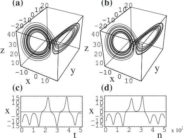
0.0237, respectively, which indicates that no overfitting occurs. Figure 4 shows the evolutions of the original and neural systems, starting at the same initial condition. The point where both systems start splitting away (≈t= 3) is approximately the threshold value imposed by the chaotic behavior in the numerical precision of the performed computations; therefore, it can be qualitatively stated that both systems behave similarly.

0 1 2 3 4 5

-15 -10 -50 5 10 15

0 1 2 3 4 5

-15 -10 -50 5 10 15 -10 0 10 -20 -10 0 10 20 10 20 30 40 -10 0 10 20 -10 0 10 20 -10 0 10 -20 -10 0 1020 10 20 30 40 -10 0 10 20 -10 0 1020

(a)

(b)

(c)

(d)

z

x

y

z

x

y

x

x

t

n

2

Figure 4: Phase and evolution spaces of (a) the Lorenz model and (b) an approximate neural model with 15 hidden neurons.

have seen that most of the times the neural models asymptotically diverge to infinity). As a conclusion, a commitment between error minimization and dynamical reconstruction leads to optimal neural models ranging from 10 to 20 hidden neurons.

From the above experiments we have seen that the residual training or test errors do not provide a general criterion for determining a similar dynamical behavior between a given dynamical system and a neural approximate model. In the following sections we shall give such a criterion based on chaos synchronization; in this case we do not compare the prediction error, but the synchronization error between the systems.

3

Chaos Synchronization

In their seminal contribution Pecora and Carroll [17] showed that chaotic systems can be synchronized by linking them with common signals. At first sight, this is not an obvious result, since these systems are very sensitive to small perturbations on the initial conditions and, therefore, close orbits of the system quickly become uncorrelated. They consider the situation of unidirectional driving in which one has a couple of master-slave systems, and synchronization is achieved by injecting a signal from the master system into the slave.

Given a couple of identical autonomous chaotic systems, ˙u₁ = f(u₁) and ˙u₂ = f(u₂), the basic idea of the Pecora-Carroll scheme is decomposing the first system (the master) into two subsystems,

˙

v1 =g(v1,w1)

˙

w1 =h(v1,w1)

)

master, (3)

where u = (v,w), and considering one of the decomposed subsystems as master signal, say v1, to be injected into the slave system. This reduces the dimensionality of the slave becoming

˙

w₂ =h(v₁,w₂)} response, (4)

where v1 is the set of connecting variables. Note that the system (3) is independent of the

response system, whereas (4) is driven byv1(t) (unidirectional driving). Then, the question is

whether or not the subsystemsu1 andu2 will synchronize, i.e., whetherku1(t)−u2(t)k →0,

ast→ ∞. The answer to this question is given by the Lyapunov exponents of the difference system, ˙δw=h(v1,w1)−h(v1,w2), since they indicate if small displacements of trajectories

are along stable or unstable directions. In the case of the Lorenz system these exponents are all negative when using x or y variables as driving signals, indicating that synchronization occurs.

0 200 400 600 800 1000 1200 1400 -0.2

-0.1 0 0.1 0.2

0 200 400 600 800 1000 1200 1400 -0.2

-0.1 0 0.1 0.2

0 200 400 600 800 1000 1200 1400 -0.2

-0.1 0 0.1 0.2 -15 -10 -5 0 5 10

15

(a)

n

s

n

(b)

(c)

(d)

m

n

s

n-m

n

s

n-m

n

s

n-m

n

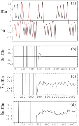
Figure 5: (a) Evolution ofxvariable for mastermnand slavesnsystems before and after

syn-chronization; (b) synchronization error with two identical systems; (c) synchronization error with a perturbed slave system ¯sn; and (d) synchronization error with a neural approximate

Pecora and Carroll also showed that synchronization is robust to small perturbations on the system parameters (this situation is usually referred to as inhomogeneous driving); in this case the trajectories do not exactly match each other, but there is a residual error associated with the differences between the systems’ parameters. For instance, Figure 5(c) shows the synchronization error resulting when considering a slave which is a slighted perturbed copy of the master system (the slave parameters have been randomly perturbed a 5% of their magnitude). From this figure we can see that the synchronization error is two orders of magnitude lower than the range of the corresponding x variable.

Finally, Figure 5(d) shows the synchronization error when considering as slave system the 15-neuron NN described in the previous section, obtained for approximating the dynamical behavior of the master system (1). The synchronization error is similar to the obtained in the previous case, when synchronizing the 5% perturbed slave system. Therefore, if we consider the residual synchronization error as a quantitative dynamic-similarity measure, we may argue that both the neural and perturbed systems are similar dynamical approximations of the original driving system.

4

Dealing with Experimental Time Series

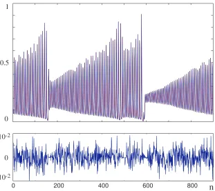
The above ideas can be applied in a great variety of domains where nonlinear time series associated with problems of interest are available. However, a common problem with many of these time series is that they only represent a single scalar measurement of the system. For instance, Figure 6 shows a time series corresponding to a single scalar measurement (the intensity) of a N H3 infrared laser (this time series was used in the Santa Fe time series prediction competition [20]).

When the time series is obtained by sampling a single coordinate, say x, one can still obtain a faithful phase-state representation of the dynamics by considering, for example, the delay reconstruction space method [7] and taking as new coordinates the values xi, xi−τ, xi−2τ, . . . , xi−d τ, where the parameters τ (the delay factor) and d (the dimension of

the delay embedding space) can be obtained from the time series. Using the mutual in-formation of the time series we obtained a value τ = 10 and applying the method of false neighbors we obtained a valued = 6. Therefore, we considered a NN with 6 input neurons, (xn−10, xn−20, . . . , xn−60), and a single output neuronxnfor approximating the dynamical

sys-tem underlying the time series. Figure 6 shows the training errors obtained with a 6 : 5 : 5 : 1 neural network.

0.5

0 1

0 200 400 600 800

_n

-10-2

10-2

0

0.5

0 1

800 1000 1200

_n

Laser

Neural

Figure 6: Time series corresponding to the intensity of aN H3 infrared laser (above); training errors for a 6 : 5 : 5 : 1 neural network (below).

Figure 7 shows the result obtained when applying the above algorithm using the laser time series as master system and the neural model as slave. This figure clearly shows that synchronization is quickly achieved, indicating that the neural model is a good approximation of the dynamical system underlying the data.

References

[1] Brillinger, D.R. (1981) Time Series. Data Analysis and Theory. McGraw-Hill.

[2] Lorenz, H.W. (1997) Nonlinear Dynamical Economics and Chaotic Motion. Springer-Verlag.

[3] Pecora, L. M., editor (1993) Chaos in communications SPIE Proceedings Vol. 2038.

[4] R.M. May (1987) Chaos and the dynamics of biological populations, Proceedings of the Royal Statistical Society, A413.

[5] Farmer, J.D. and Sidorowich, J.J. (1987) Physical Review Letters, 59, 845.

[6] Stern, H.S. (1996) Technometrics, 38(3), 205.

[7] Packard, N.H., Crutchfield, J.P., Farmer, J.D. and Shaw, R.S. (1980) Physical Review Letters, 45, 712.

[8] Meyer, Y. and Ryan, R.D. (1991) Wavelets. Algorithms and Applications.

[9] Castillo, E., and Guti´errez, J.M. (1998) Nonlinear time series modeling and prediction using functional networks. Extracting Information masked by chaos. Physics Letters A,

244, 71–84.

[10] Kantz, H. and Schreiber, T. (1997) Nonlinear Time Series Analysis. Cambridge Univer-sity Press.

[11] Nakendra, K.S., and Parthasaraty, K. (1992) Neural networks and dynamical systems. International Journal of Approximate Reasoning, 6, 109–131.

[12] Greenwood, G.W. (1997) Training Multiple-layer perceptron to recognize attractors. IEEE Transactions on Evolutionary Computation, 1, 244–248.

[13] Principe, J.C., Rathie, A., Kuo, J.M. (1992) Prediction of chaotic time series with neural networks and the issue of dynamic modeling. International Journal of Bifurcation and Chaos, 2, 989–996.

[15] Cheng, G., Cheng, Y., and Ogmen, H. (1997) Identifying chaotic systems via a Wiener-type cascade model. IEEE Control Systems, October, 29–35.

[16] Guti´errez, J. M. and lglesias, A. (1998) A Mathematica Package for the Analysis and Control of Chaos in Nonlinear Systems, Computers in Physics, 12(6), 608-619.

[17] Pecora, L.M. and Carroll, T.L. (1990) Physical Review Letters, 64, 821.

[18] Cybenko, G. (1989) Approximation by Supperpositions of a Sigmoidal Function. Math-ematics of Control, Signals, and Systems, 2, 303-314.

[19] Lorenz, E.N. (1963) Journal of Atmospheric Sciences, 20, 130.

[20] Weigend, A., Gershenfeld, N.A., editors (1993) Time Series Prediction: Forecasting the Future and Understanding the Past, Addison-Wesley.