Christoph Ortner Based on Lecture Notes by John Ball

(1)

Solid Mechanics

Christoph Ortner

Based on Lecture Notes by John Ball

ortner@maths.ox.ac.uk

Mathematical Institute, 24-29 St. Giles’, Oxford, OX1 3LB

(2)

1 Introduction

Solid mechanics is the branch of mechanics, physics and mathematics that concerns the behaviour of solid matter under external actions such as external forces, temper-ature changes, etc.. Typically, a solid body has a rest shape (the reference config-uration) and one studies the departure (the deformation) from this rest shape. For moderate applied loads most solids behave elastically, that is, after a load is removed it returns to its original shape. This deformation regime is described by the theory of elasticity, which is the backbone of solid mechanics and the main focus of this course. Phenomena beyond the theory of elasticity include plastic deformation and fracture and will only briefly be touched upon.

This course will focus on a careful and fairly rigorous (that is, a definition-theorem-proof style) derivation of the theory of elasticity from basic continuum me-chanics concepts. This will be followed by various illustrative examples, a derivation of linearised elasticity, incompressible elasiticty, and brittle fracture.

1.1 Literature & Acknowledgements

In preparing these lecture notes I have largely followed the structure of the course previously taught by John Ball and his lecture notes [Bal], but have modified/adapted specific parts following the books of Ciarlet [Cia88], Gurtin [Gur81a, Gur81b], and Gonzalez & Stuart [GS08]. In particular, most of the examples and exercises are taken (with only small variations) from [Bal].

Gurtin’s notes [Gur81b] will give a very concise introduction into the modelling of solids, but lack detail. The books of Gurtin [Gur81a] and Gonzalez & Stuart [GS08] provide unified introductions into continuum solid and fluid mechanics. I find that Gonzales & Stuart provide particularly clear motivations of many continuum mechanics concepts.

Ciarlet’s book [Cia88] focuses exclusively on solids and goes much deeper into the mathematical theory than any of the other references. It is highly recommended for further studies into the field of mathematical elasticity, but may be too dry and technical for a first course.

The material on incompressible elasticity is a subset of the presentation in [Bal]. The presentation of linear elasticity is standard and can be found in similar forms in many texts. Finally, the presentation of brittle fracture is a combination of a few classical ideas that are presented in similar form in various texts, together with a brief outline of the recent variational theory.

2 Prerequisites

(5)

2.1 Linear Algebra

The space of real n-vectors is denoted Rn_{, with canonical basis} _e

1, . . . , en. The space

of real m×n- matrices is denoted Mm×n_{. The identity matrix is denoted} ₁_{. The}

sets of orthogonal matrices and proper orthogonal matrices (rotations) are denoted, respectively, by

O(n) = Q∈Mn×n_:_QT_Q₌_QQT ₌₁ _, _and

SO(n) = Q∈O(n) : detQ= 1 .

The notation for volume and area is as follows: if A ⊂ Rn _{has a well-defined}

volume (i.e., Lebesgue measure), and ifB ⊂Rn _{is a surface with well-defined surface}

area (e.g., piecewise C1_{-hypersurface), then}

vol(A) =:|A| and area(B) =:|B|

denote, respectively, the volume of A and the area of A.

2.1.1 Norms and inner products

The Euclidean norm is denoted

|x|=

n

X

i=1

|xi|2

₁_/₂

for x∈Rn_.

The associated inner product is given by

hx, yi=xT_y₌Xn i=1

xiyi =xiyi for x, y ∈Rn.

The last form above uses the summation convention, which we will employ liberally whenever convenient.

The Frobenius norm of a matrix is

|T|=

m

X

i=1

n

X

α=1

|Tiα|2

₁_/₂

forT ∈Mm×n_.

The associated inner product is normally denoted

T :S =

m

X

i=1

n

X

α=1

TiαSiα =TiαSiα = tr(TTS) for S, T ∈Mm×n.

(6)

2.1.2 Tensor and cross product.

The tensor (or outer) product of two vectors a ∈ Rm_{, b} _∈ _Rn _{is the matrix} _a_⊗_b _∈

Mm×n_,

a⊗b=abT _{= (}_a

ibj)i=1,...,m j=1,...,n

It is sometimes better understood as the linear operator with the action (a⊗b)h = (b·h)a for h∈Rn_.

The cross product (or exterior product) of two vectors a, b ∈ R3 _{is the vectors}

a×b ∈R3_,

a×b=



 a_a2₃b_b₁3−₋a_a₁3_bb2₃ a1b2−a2b1

 

Two non-zero vectors a, b are parallel if and only if a×b = 0. If a and b are not parallel then, geometrically, a×b is the unique vector that is (i) orthogonal to a

and b; (ii) the three vectors a, b, a×b (in that order) form a right-handed coordinate system (possibly non-orthogonal); and (iii) |a×b| is the area of the parallelogram spanned by a, b.

(Remark: The × product is also denoted ∧, particularly its generalizations to

higher dimensions and in differential geometry.)

2.1.3 Eigenvalues and eigenvectors of symmetric matrices

If A ∈ Mn×n _{is symmetric then there exist} _n _eigenvalues _λ

i ∈ R with associated

normalized eigenvectors qi ∈Rn, |qi|= 1, i= 1, . . . , n, such that

Aqi =λiqi.

The eigenvectors form an orthonormal basis of Rn_{, that is,}

A=Xn

i=1

λiqi ⊗qi, or, equivalently, A=QΛQT,

where Λ = diag(λ1, . . . , λn) and Q= (q1, . . . , qn) is orthogonal.

2.1.4 The cofactor matrix

Let A ∈ Mn×n_{, and let} _A0

i,j be the submatrix of A in which the i-th row and j-th

column are removed. Then the cofactor matrix cofA is defined as cofAn_i,j₌₁ = (−1)i+j_det_A0

i,j

_n

i,j=1.

The cofactor matrix satisfies the relations

(7)

in particular, ifA is invertible, then

cofA= (detA)A−T_.

(Remark: Some authors prefer to introduce the adjugate adjA= (cofA)T _instead

of the cofactor matrix.)

2.1.5 The orientation tensor

The orientation tensor (or Kronecker symbol; or Levi-Civita symbol; . . . ) is the third-order tensor defined by

ijk =

  

1, if ijk is an even permutation of 123,

−1, if ijk is an odd permutation of 123,

0, otherwise.

=

  

1, if ijk ∈ {123,231,312},

−1, if ijk ∈ {321,213,231},

0, otherwise.

Amongst other things, it provides useful formulas for the cofactor and the determi-nant. Let A= (Aiα)3iα=1 ∈M3×3, then

(cofA)iα = 1₂ijkαβγAjβAkγ, and

detA= 1

6ijkαβγAiαAjβAkγ.

Moreover, the cross product of two vectors a, b∈R3 _{can be expressed as follows:}

(8)

2.2 Calculus

2.2.1 Differentiation

A connected open set U ⊂ Rn _{is called a domain. A function} _f _:_U _→_Rm _{is said to}

be (Fr´echet-)differentiable at a point x∈ U, if there exists a matrix ∇f(x)∈ Rm×n

(the Jacobi matrix) such that

f(x+h) = f(x) +∇f(x)h+o(|h|),

where o : [0,+∞) → [0,+∞) satisfies limt&0o(t)/t = 0. The components of ∇f(x)

are the partial derivatives

∇f(x) = ∂xjfi

i=1,...,m

j=1,...,n. (1)

(∇f is often denoted Df instead. Some texts will then define ∇f =DfT_{. Here, we}

will use the notation ∇f throughout and stress that in (1) i is the row index and j

the column index.)

When it is clear with respect to which variable the differentiation is understood then we will sometimes write

fi,j =∂xjfi,

that is, the comma separates the component index from the differentiation idex.

2.2.2 Divergence and divergence theorem

LetU be a domain with piecewise smooth boundary so that the outward unit normal

N is well-defined, and let f : U → Mm×n _{be continuous differentiable in} _U_{, and}

continuous on ¯U. Then the divergence theorem states that

Z

∂UfNdA =

Z

∂UfiαNαdA =

Z

U∂xαfiαdV =

Z

UDivfdV,

where

(Divf)i = n

X

α=1

∂xαfiα =∂xαfiα =fiα,α.

We note here, that dV denotes the volume element and dA denotes the area element. If we want to stress that the integration is performed with respect to the

x-variable, then we will write dVx or dAx instead.

2.2.3 Change of variables

Let U ⊂ Rn _{be a domain and let} _y _: _U _→ _R3 _{be continuously differentiable and}

bijective (a diffeomorphism), then

Z

Uf(x) dVx =

Z

Uy

(f ◦y−1₎₍_ϕ_)|(det∇_y−1₎₍_ϕ_)|_dV

(9)

where Uy _:=_y₍_U_{) denotes the “deformed domain”.}

If y is a deformation of a body Ω ⊂ R3_{, and} _E _{a part of Ω (cf. Section 3) then}

we normally write _Z

EfdV =

Z

Ey

f|det∇y−1_|_dv_. ₍₂₎

(10)

Part 1: Modelling 3D Elasticity

3 Kinematics

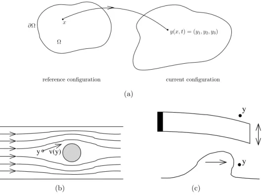
3.1 Reference and deformed configuration.

A body occupies a region in Euclidian space R3_{. Although it may occupy different}

regions at different times, it is convenient to fix one such region Ω, say, which we call

thereference configuration, and to identify the body with this region. We will assume

throughout that Ω is open and connected (i.e., a domain) with a sufficiently smooth boundary (i.e., the boundary can locally be described as the graph of a function that is at least Lipschitz continuous, but possibly smoother). Each point x∈ Ω is called

amaterial point. The assumption that Ω is open is made primarily for mathematical

convenience.

Mathematically, a body is deformed via a mapping y taking a material point x

to a point y(x) in space. Such a mapping should have the following properties, each of which we address in more detail below:

1. We assume that y is “sufficiently smooth”, normally at least differentiable. 2. No two material points may occupy the same position in space at the same

time, that is,y : Ω→R3 _{must be one-to-one. However, to allow contact, we do}

not require that y: ¯Ω→R3 _{is one-to-one. (see Figure 1)}

3. The map should be orientation preserving. We will return to this below, but note already now that, mathematically, this is expressed by the condition that det∇y(x)>0 (where ∇y(x) is the deformation gradient; see Sec. 3.2)

We call a “sufficiently smooth”, invertible and orientation preserving mapy : Ω→R3

a deformation. The set y(Ω) is called the deformed configuration. For notational

convenience we will usually denote it Ωy _:=_y_{(Ω). We will see in Section 3.3 that, if}

y is smooth and orientation preserving then Ωy _{is again a domain.}

Any subdomain E ⊂ Ω is called a part of Ω (or, of the body). Throughout, we will use the notation Ey ₌_y₍_E_{) to denote parts of the deformed body. Since parts}

of Ω and of Ωy _{are related one-to-one (cf. Sec. 3.3), this is not an abuse of notation.}

3.2 The deformation gradient.

One of the main (simplifying) features of continuum mechanics is that a body can be divided into arbitrarily small pieces. Thus, if a deformationyis smooth (normally at least differentiable) then it can be locally approximated by an affine map, that is,

(11)

by the solid at any time in a given motiony.

Notation. We use Greek indices for the coordinatesxαand Latin indices for the

coordinatesyi.

Thedeformation gradient is the differential ofywith respect tox, denoted

F =Dy; Fiα=yi,α= _∂x∂yi α.

Invertibility

To avoid interpenetration of matter, we require that for eacht,y(·, t) is invertible on Ω, with sufficiently smooth inversex(·, t). We also suppose that y(·, t) is orientation preserving; hence

J = detF(x, t)>0 forx∈Ω. (1)

By the inverse function theorem, (1) implies thaty(·, t) is locally invertible. Examples.

not on Ω

locally invertible but not globally invertible

y

y(·, t) invertible on Ω

y

Everting a sphere (Smale) can be done without violating local invertibility (see the videohttp://video.google.com/videoplay?docid=-6626464599825291409.

How can we verify thaty(·, t) is invertible? A useful result for the case when there is no self-contact is

4

(a) by the solid at any time in a given motiony.

Notation. We use Greek indices for the coordinatesxαand Latin indices for the

coordinatesyi.

Thedeformation gradientis the differential ofywith respect tox, denoted

F=Dy; Fiα=yi,α=_∂x∂yi α.

Invertibility

To avoid interpenetration of matter, we require that for eacht,y(·, t) is invertible on Ω, with sufficiently smooth inverse x(·, t). We also suppose thaty(·, t) is orientation preserving; hence

J= detF(x, t)>0 forx∈Ω. (1)

By the inverse function theorem, (1) implies thaty(·, t) is locally invertible.

Examples.

not on Ω

locally invertible but not globally invertible

y

y(·, t) invertible on Ω

y

Everting a sphere (Smale) can be done without violating local invertibility (see the videohttp://video.google.com/videoplay?docid=-6626464599825291409.

How can we verify thaty(·, t) is invertible? A useful result for the case when there is no self-contact is

4

(b)

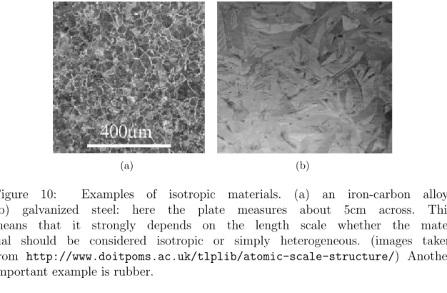
Figure 1: (a) A deformation that is locally invertible but not globally invertible. (b) A deformation that is invertible on Ω but not on ¯Ω (contact)

where the matrix field F : Ω→M3×3_,

F(x) = Dy(x) = ∂xαyi(x)

₃

i,α=1

is called thedeformation gradient. (In this notation,i is the row index whileα is the column index.)

The symbol o(t), t > 0 means that limt&0o(t)/t = 0. Thus, (3) is in fact the

definition of (Fr´echet-)differentiability of y.

A deformation is called homogeneous if F(x) is constant, that is, y(x) =a+F x

for some constants a∈R3 _and _F _∈_M3×3_.

The approximation (3) allows us, for many questions, to concentrate entirely on infinitesimal parts of the body where the deformation can be considered an affine map, that is, a homogeneous deformation. We will return to this point in Section 4.

3.3 Orientation preserving maps, invertibility.

(12)

(b)

A B

C D

A B

C D

D C

B A

(a)

Figure 2: Two deformations of a cube. (a) orientation preserving, det∇y > 0 (b) reversing the orientation, det∇y <0.

In general, we will always require that the deformationyisorientation-preserving, that is,

J(x) := detF(x)>0 ∀x∈Ω (4) An immediate consequence of (4) and the inverse function theorem Theorem 3.1 below is that such a map is locally invertible and open, that is, it maps open sets to open sets.

Theorem 3.1 (Inverse function theorem). Let A⊂Rn _{be open,} _f _∈_C1₍_A_;_Rn₎_,

and x0 ∈ A. If ∇f(x0) is invertible then there exists an open neighbourhood U of

x0 such that f(U) is open and f : U → f(U) is a diffeomorphism. Furthermore,

∇f−1₍_f₍_x

0)) = (∇f(x0))−1.

In addition to the condition that a deformation is orientation-preserving, we also require that it is invertible, that is, no two material points may occupy the same

point in space at the same time. While the condition J = detF > 0 ensures local

invertibility, it does not guarantee global invertibility (or, non-interpenetration); see Figure 1 to visualize the difference between local and global invertibility. One result that globalizes the inverse function theorem is the following.

Theorem 3.2 (A global inverse function theorem). Let Ω⊂Rn _{be a bounded}

domain with sufficiently smooth boundary and lety∈C1_(¯Ω;_R3₎_{so that}_det∇_y₍_x₎_>₀

for all x∈ ¯Ω and y|∂Ω is one-to-one. Then y is one-to-one on ¯Ω.

3.4 A note on Lagrangian and Eulerian variables

In continuum mechanics, typically one of two possible descriptions of mo-tion/deformation are used (see also Figure 3):

(i) The material (Lagrangian) description: In the material description, one fixes

(13)

ξ

v(ξ, t)

Different particles of the fluid pass throughξat different times. The Eulerian description is used mainly because in it the governing equations take a rela-tively simple form. However the description is awkward when there are free boundaries, since a pointξmay be occupied by fluid at some times, and not at others.

ξ ξ

wave on sea cavitation

For solids, it is more convenient to use theLagrangianormaterialdescription of motion, in which we fix attention on a given particle ormaterial point, of the solid (not to be confused with an atom) and study how it moves. In this description free boundaries are described automatically.

We label the material points by the positionsx= (x1, x2, x3) they occupy

in areference configuration, in which the solid occupies a region Ω⊂R3_{. We}

assume Ω is open and connected (adomain) with sufficiently smooth boundary

∂Ω. Usually we suppose Ω is bounded. Lety(x, t)∈R3_{be the position occupied}

by the material pointx∈Ω at timet.

y(x, t) = (y1, y2, y3)

Ω

∂Ω x

reference configuration current configuration

Thusy: Ω×(t1, t2)→R3, −∞!t1< t2!∞. We suppose thatyis

sufficiently smooth. Note that the reference configuration need not be occupied

3

(a)

y v(y)

(b)

y

(c)

Figure 3: Visualization of (a) the material (Lagrangian) description of motion and (b) the spatial (Eulerian) description of motion. (c) The problem of free boundaries in the spatial description.

(ii) The spatial (Eularian) description: In the spatial description of motion, we fix a

point y in space and study what occurs at that fixed point as time progresses, instead of tracking individual particles as they move through space. In fluid mechanics, this description is convenient, because the governing equations take a particularly simple form. However, it is more difficult to treat free boundaries, which is crucial in solid mechanics (see Figure 3(c). The variabley is called the

Eulerian variable.

If y is a deformation of a body Ω, then any material field, that is, a function defined on Ω can be transformed to the spatial description and vice versa, by the relation

f(x)↔f(y) = (f◦y−1₎₍_y₎_.

Here and throughout, we use the same symbols for a material field f and its corre-sponding spatial field f ◦y−1 _{(or, the spatial field} _f _{and its corresponding material}

fieldf◦y). Moreover, we use the same symbol for the deformationyand the Eulerian variable y. Even though this is a slight abuse of notation, it should always be clear from the context what we mean.

(14)

the same properties in the alternative configuration. As an example, we consider the transformation of the mass density.

Example 3.3 (Conservation of Mass). As a first simple example of relating the material and spatial descriptions, we define the notion of mass and mass density. In continuum mechanics it is typical to assume that the mass of any partE of Ω can be expressed as

mass(E) =

Z

Eρ(x) dV,

whereρ : Ω→R is called the mass density field. Theaxiom of conservation of mass

requires that, after a deformation y, the mass of the part E must remain the same, that is,

mass(y(E)) = mass(E). (5) Appealling to the change of variables formula for volume integrals (2) we obtain

Z

Eρ(x) dV =

Z

Ey

ρ◦y−1_J−1_dv_.

Hence, if we define the mass per unit volume in the deformed configuration

ρy _:=_J−1_ρ_◦_y−1 ₌_ρ/J,

then we obtain

mass(Ey_{) =}Z Ey

ρy_dv_.

(We use the superscript y in ρy _{to stress that} _ρy _{depends on the deformation} _y_{. We}

also stress that ρy ₆₌_ρ_◦_y−1_!)

3.5 Exercises

Exercise 3.1. The reference configuration of a body is given by the infinite slab

Ω = {−A < x1 < A}, whereA >0.

(a) Verify that the map

y(x) = x1+kx3, x2+kx3, x3−k(x1+x2),

where k >0, is a (homogeneous) deformation.

(b) Show that the displacement vectory(x)−x, is orthogonal to x, for anyx6= 0. (c) Show that the deformed body occupies another infinite slab, and that, as

k → ∞, the thickness of the slab tends to 2√2A, and that the angle between the normal to its faces and thex1-axis tends to π/4. Exercise 3.2. Use the global inverse function theorem to show that the map given by

(15)

e

y

(a)

e y

(b)

Figure 4: (a) A rigid body rotation about the axis e. (b) An extension, from 0, in direction e.

is a deformation (i.e., orientation preserving and invertible) of the domain

Ω = x1 >0, x2 >0,1< x1+x2 <2,0< x3 <1 .

Exercise 3.3. Letρbe the mass density in the reference configuration. LetG⊂R3 be open and bounded. Show that

ρ(x) = lim

r&0 R

x+rGρdV

r3_|_G_| .

Discuss briefly how one might use this identity to define or motivate the notion of mass density. Without being too rigorous, what kind of features does the map

E 7→mass(E) require so that the mass density is meaningful?

4 Analysis of Strain

The present section focuses on the analysis of homogeneous deformations. We begin by studying two important examples: rotations and extensions. We will then see that

all homogeneous deformations can be decomposed into deformations of these two types and translations.

(Remark: the termstrain is used for any object that measures, locally, the amount

of deformation, particularly the discrepancy from a rigid body motion. In the following we will use the term strain without further comments.)

Example 4.1 (Rotations). A deformation y(x) = Rx is a (rigid body) rotation if RT_R ₌₁ _{and det}_R _{= 1. We also call the deformation gradient} _R _{a rotation. The}

spectrum of F =R is given by

(16)

The valueθ is called theangleof the rotation and the eigenvector e=eR

correspond-ing to the eigenvalue 1 is called the axis of rotation (though this is only useful if R

is non-trivial, that is, if R6=1).

Thus, the real Jordan normal form of R (the representation in any orthonormal basis with eR as the third vector) is

R ∼



 cos(_sin(θ_θ)₎ −_cos(sin(θ_θ) 0_{) 0}

0 0 1

 

4.1 The Polar decomposition.

As announced above, all deformation gradients can be decomposed into rotations and (mutually orthogonal) extensions. This observation is based on two simple tools from linear algebra that we develop next.

Lemma 4.3 (Square roots of matrices). Let C ∈ Mn×n _{be a symmetric and}

positive definite (spd) matrix. Then there exists a unique spd matrix U such that

C =U2_,

and we write U =C1/2 ₌√_C_.

Proof. Since C is symmetric, it admits the spectral decomposition

C =Xn

i=1

λiqi⊗qi.

Setting

U =

n

X

i=1 p

λiqi⊗qi,

we obtain

U2_q

j =U(

p

λjqj) = (

p

λj)2qj =λjqj forj = 1, . . . , n.

(17)

To prove the uniqueness, let ˆU be any spd matrix such that ˆU2 ₌_C_{. Then}

ˆ

U2_q

i =Cqi =λiqi,

in particular, {q1, . . . , qn} is an eigenbasis for ˆU2. But this implies that it is also an

eigenbasis for ˆU. If ˆλi are the corresponding eigenvalues then it follows immediately

that ˆλ2

i =λi and since ˆU was spd, this means that ˆλi =√λi, that is, ˆU =U.

Remark 4.4. Taking the square root of a matrix commutes with taking its inverse. Thus, we will usually write (C1/2₎−1 _{= (}_C−1₎1/2 ₌_C−1/2_._(exercise)

Lemma 4.5 (Polar decomposition). Let F ∈Mn×n_, _det_{F >}₀_{, then there exist}

unique matrices U, V, R ∈ Mn×n _{such that} _U _and _V _{are spd and} _R _∈ _SO(_n₎_{, and}

such that

F =RU =V R.

Proof. Suppose such a decompositions exist, then

FT_F ₌_UT_RT_RU ₌_U2_, _{and similarly} _{F F}T ₌_V2_.

It is easy to see that FT_F _and _{F F}T _{are positive definite, and hence, by Lemma 4.3,}

U and V satisfying the above equations exist and are unique. Let R=F U−1_{, then}

RT_R ₌_U−1_FT_{F U}−1 ₌_U−1_U2_U−1 ₌₁_,

hence R is orthogonal. To show that detR >0, we note that 0<detF = detRdetU.

Since detU > 0, it follows that detR >0. Finally, we note that

F =RU = (RURT₎_R.

Since this representation is unique, it follows thatV =RURT_{, and in particular that}

F =V R.

4.2 The stretch tensors and the Cauchy–Green strain

ten-sors.

Let F = ∇y be a deformation gradient (either homogeneous or space-dependent), and letF =RU be its right polar decomposition. SinceU is symmetric, we can write it in the form

U =

3 X

i=1

(18)

where qi and λi are the eigenvectors and eigenvalues ofU, and

Ui =1+ (λi−1)qi⊗qi;

(the above identify is easily verified). Thus, the matrices U1, U2, U3 represent simple

extensions in mutually orthogonal directions, and we obtain, in summary,

F =RU3U2U1, (6)

which is the statement announced at the beginning of the section. It is also easy to see that the matricesUi commute, that is, the order in which the stretches are applied

does not matter. The eigenvalues λi are called the principal stretches. The matrices

U and V (whereF =RU =V R) are called the right and left stretch tensors.

We will later see that rotations do not affect material response, but only the stretch tensors are important. These are, however, difficult to compute in general and it is usually more convenient to work with the so-called right and left Cauchy– Green strain tensors

C =FT_F ₌_U2 _and _B ₌_{F F}T ₌_V2_,

Apart from the principal stretches, the principal invariants of U, V, C, B will also be important later on. These are introduced in the exercises in the following section.

4.3 Exercises

Exercise 4.1. Compute the positive square roots of the following matrices:

(i)

5 0 0 15

(ii)

3 −1 −1 3

(iii)



 ₋₄5 −4₆ ₋₄1

1 −4 5



_.

Exercise 4.2. Find the left and right polar decompositions of the following matri-ces:

(i)

2 −3 1 6

and (ii)

 

√

2 −1 1 √

2 1 −1

0 1 1



_.

Exercise 4.3. LetF =RU be the (right) polar decomposition ofF ∈M3×3. Show that |R−F| <|Q−F| for all Q ∈SO(3), Q6=R. (Hint: Consider the case when F

is diagonal and positive.)

Exercise 4.4. LetS ∈M3×3 then det(S−ω1) admits the representation det(S−ω1) =−ω3₊_I

(19)

where IS, IIS, IIIS are the principal invariants of S.

(a) If S is symmetric with eigenvalues λ1, λ2, λ3, prove that

IS =λ1+λ2+λ2, IIS =λ1λ2+λ2λ3+λ3λ1, and IIIS =λ1λ2λ3.

Show also that this relation between eigenvalues and principal invariants is invertible. (b) Deduce that

IS = trS, IIS = 1₂(trS)2−tr(S2) = tr(cofS), and IIIS = detS.

(c) If S =C is the right Cauchy–Green strain tensor, show that

IC =|F|2, IIC =|cofF|2, and IIIC = (detF)2.

(d) Show that IC = IB, IIC = IIB, and IIIC = IIIB, where B is the left Cauchy–

Green strain tensor.

Exercise 4.5. A homogeneous deformation of the form

y(x) = x1+γx2, x2, x3

is called a pure shear (or simple shear).

(a) Calculate the principal stretches and show that the right polar decomposition of F =∇y is given by

F =RU =



 ₋cos_sinψ_ψ _cossinψ_ψ 0₀

0 0 1

 



 cos_sinψ_ψ 1+sinsin2ψ_ψ 0

cosψ 0

0 0 1

 _,

where tanψ = 1

2γ. Also find the left polar decomposition.

(b) Let ei denote the canonical basis vectors. Show that, as γ → 0+, the

eigen-vectors of U and V tend to

1 √

2(e1+e2), √12(e1−e2), and e3.

Hence, visualize the infinitesimal displacement as γ →0+.

5 The Stress Principle of Euler and Cauchy

(20)

5.1 Forces

The interaction between parts of a body, or the body and the outside world, is described by forces. In this section, we will describe the different types of forces acting on (parts of) a body.

5.1.1 Body forces

External body forces are defined by a vector field

by _{: Ω}y _→_R3_,

called thedensity of applied force per unit mass in the deformed configuration. If Ey

is a part of Ωy _{then the resultant force acting on} _Ey _{due to the body force field is}

Z

Ey

by₍_y₎_ρy₍_y_{) dv}

The resultant torque on Ey_{, about a point}_z_{, is}

Z

Ey(y−z)×b

y₍_y₎_ρy₍_y_{) dv}_.

The prototypical example of a body force is the gravity fieldby₍_y_{) =} ₋_ge

3, where

g is the gravitational constant. Other examples are magnetic or electric forces.

5.1.2 Surface forces

The forces arising due to physical contact between bodies are called surface forces. This includes the forces due to contact between the body Ω and an external body

(external surface forces), but also the forces acting between parts of Ω (internal

surface forces).

Let Ey _{be a (smooth) part of Ω with outward unit normal} _n _at _∂Ey_{. Then the}

force per unit area, exterted by the material on the “outside” of Ey _{on the material}

upon the “inside” is a functionsEy :∂Ey →R3, called thetraction fieldor thesurface

force field for∂Ey_.

The resultant force due to a traction field on the surface ∂Ey _is

Z

∂EysE

y(y) da, and the resultant torque, about a point z, is

Z

∂Ey

(y−z)×sEy(y) da.

As indicated above, we will consider two types of traction fields: internal and external. The external traction field is defined on ∂Ωy _{and is denoted}

(21)

This describes the traction on a body produced by an external body that is in contact. Note that, so far, the internal traction field for a given surface, may depend on this surface in any possible fashion. The stress principle of Euler and Cauchy postulates a very concrete form for the traction field due to the internal forces.

Axiom 5.1 (Stress principle of Euler and Cauchy). Let y be a deformation of

Ω. Then there exists a vector field s : ¯Ωy _×_S

1 → R3 (the Cauchy stress) such that,

for any smooth part Ey _⊂ _Ωy _{with outer unit normal} _n_, _s₍_{y, n}₎ _{is the traction field}

for the surface ∂Ey _{due to the internal forces, i.e.,} _s

Ey(y) =s(y, n) on ∂Ey.

Remark 5.2. The stress principle of Euler and Cauchy is a simplifying assumption on the nature of traction on a surface. It not only postulates that traction is a local

property, but also that it depends only on the unit normal to a surface, and not, for example, on the curvature, and so forth. It is not obvious that this assumption is always justified. It relies, in essence, on the short interaction range of the forces acting between the atoms (or other building blocks) of a body, and on the assumption that the surfaces under consideration are smooth, which means that, locally at the microscopic level, they can be considered affine. However, if the orientation of a sur-face varies rapidly in relation to the atomic scale (for example) then this assumption

must be considered inaccurate.

By an approximation argument, whereby parts with piecewise smooth boundaries (e.g., polyhedra) are approximated by smooth sets, the Cauchy stress is also defined for piecewise smooth partsEy_{. In that case, the outward unit normal is not defined in}

all points of ∂Ey_{, but in all points except the edges or corners between the smomoth}

portions of the boundary.

In view of the previous remark, we might argue that edges and corners are neg-ligible in comparison to surfaces and hence, for sufficiently large parts Ey _(relative

to the microscopic structure) the stress principle of Euler and Cauchy should still apply.

From here on, we will always implicitly assume that the domain Ω, the deformed domain Ωy _{and their parts are piecewise smooth. Moreover, we will implicitly always}

exclude the edges and corners where normals are not defined.

5.1.3 Balance of forces

The deformed body (or, the deformation y) is a static equilibrium if the total force and the total torque are balanced for each part of Ωy_:

(i) Balance of force: For all partsEy _⊂_Ωy_,

Z

Ey

by₍_y₎_ρy₍_y_{) dv +}Z ∂Ey

s(y, n) da = 0 (8)

(ii) Balance of torque: For all parts Ey _⊂_Ωy_,

Z

Ey

y×by₍_y₎_ρy₍_y_{) dv +}Z ∂Ey

(22)

Remark 5.3. The dynamic version of (8) isconservation of linear momentum and the dynamic version of (9) is conservation of angular momentum; see also exercise

5.1.

The postulates of force and torque balance will provide equilibrium conditions in the interior of the body. On the boundary, the only condition we have available is that the Cauchy stress must match the external traction field (law of action and reaction), that is,

s(y, n) = gy₍_y₎ _∀_y_∈_∂_Ω_. ₍₁₀₎

5.2 The Cauchy stress tensor.

The following central result of continuum mechanics summarizes the consequences of the force balance axioms (8) and (9).

Theorem 5.4 (Cauchy’s Theorem). Let y be a deformation of Ω which is in

static equilibrium, and suppose also thatby_, _ρy_, _gy_{, and}_s _{are continuous. Then there}

exists a continuous tensor (or matrix) fieldS: Ωy _→_M3×3 _(the_{Cauchy tensor}_{), such}

that

s(y, n) =S(y)n ∀y∈Ω ∀n ∈S1, (11)

S(y)T ₌_S₍_y₎ _∀_y_∈_Ω_, ₍₁₂₎

Ifs(·, n)is continuously differentiable for any n, thenS is continuously differentiable,

and

divS+by_ρy _{= 0}_, _in _Ωy_. ₍₁₃₎

Proof. The proof is divided into three steps: 1. existence of the Cauchy tensor (11) (a

consequence of force balance); 2. balance of force (13); and symmetry of the Cauchy tensor (12) (a consequence of torque balance).

For simplicity, we defined ˜b=by_ρy_{, which is also continuous.}

1. Proof of (11). Fix z0 ∈ Ωy, and let G ⊂ R3 be a bounded open set with

piecewise smooth boundary, then, for ε sufficiently small, the set Ey ₌ _z

0 +εG in

contained in Ωy_{. Hence, the balance of forces (8) reads}

Z

Ey

by_ρy_{dv +}Z ∂Ey

s(y, n) da

Since ˜b was assumed to be continuous, and since |Ey_|₌_O₍_ε3_{) as} _ε_→_{0, we have}

Z

∂Eys(y, n) da

(23)

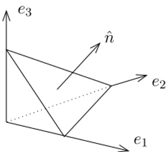
e1

e2

e3

ˆ n

1

Figure 5: The tetrahedron used in the proof of Theorem 5.4. The face opposite ej

is denoted Fj, the face opposite 0 is denoted F0. The normal to the faces Fj is −ej,

while the normal to F0 is N.

We now change variables on the left-hand side. Lety =z0+εz, then Z

∂Eys(y, n) day =ε 2Z

∂Gs(z0+εz, n) daz,

wheren now denotes the outward unit normal to∂G.(Strictly speaking we have not talked about transforming surface integrals yet, but for this uniform linear transform the transformation rule is obvious; see also Exercise 6.2.)

Dividing by ε2_{, and letting} _ε_→_{0, we arrive at} Z

∂Gs(z0, n) daz = 0.

We will obtain (11) by a judicious choice of the set G. Fix some unit vector ˆn ∈ S1

with components ˆni >0,i= 1,2,3, and letGbe the tetrahedron displayed in Figure

5. Thus, we obtain that

|F0|s(z0,nˆ) + 3 X

i=1

|Fi|s(z0,−ei) = 0.

If G is scaled to that |F0| = 1 then it is a simple exercise to show that the area of

the remaining faces is|Fi|= ˆni. Hence, we have

s(z0,nˆ) =− 3 X

i=1

s(z0,−ei)ˆni.

Letting ˆn→ej, we find that

s(z0, ej) = −s(z0,−ej), j = 1,2,3, (14)

and in particular,

s(z0,nˆ) = 3 X

i=1

(24)

where S(z0) = (s(z0, e1),s(z0, e2),s(z0, e3)).

This proves (11) for the case ˆni >0,i= 1,2,3. The argument can now be repeated

for any unit vector, always using (14) to arrive at the final form (15). Thus, we have shown (11) for all y∈Ωy _{and all}_n _∈_S

1.

Step 2: Proof of (13). In step 1, we have found that

S(y) = s(y, e1),s(y, e2),s(y, e3).

Clearly, if s is continuous then S is continuous. Moreover, if s(y, n) is continuously differentiable with respect to the y component, for fixed n, then S is continuously differentiable. Again, let Ey _⊂_Ωy_{, then the balance of force in terms of the Cauchy}

tensor S reads Z

Ey

˜_b₍_y_{) dv +}Z

∂Ey

S(y)nda = 0.

Integration by parts on the second term on the left-hand side yields

Z

Ey

_˜

b+ divSdv = 0.

Since ˜b and divS are continuous, we can divide by|Ey_| _{and let the volume shrink to}

zero to obtain (13).

Step 3: Proof of (12). For simplicity, we assume that Sis differentiable. Again,

let Ey _{be a part of Ω}y_{, so that the condition of torque balance, using the results of}

steps 1 and 2, reads

Z

Ey

y×(divS) dv =

Z

∂Ey

y×(Sn) da,

or, in index notation,

Z

Eyijkyj∂y`(S)k`dv =

Z

∂Eyijkyj(S)k`n`da. Integrating by parts on the right-hand side we obtain

Z

Ey

ijkyj∂`(S)k`−∂`(yj(S)k`)dv =−

Z

Ey

ijk∂`yj(S)k`dv = 0.

Upon letting|Ey_| _{shrink to a point, and since} _∂

`yj =δj`, this holds if and only if

ijk(S)kj = 0 in Ω.

This is, however, equivalent to S=ST_.

Taken together, (10), (12), and (13) constitute theequations of equilibrium in the

deformed configuration:

−divS= by_ρy_, _{in Ω}y_,

ST ₌ _S, _{in Ω}y_, _and

Sn= gy_, _on_∂_Ωy_.

(25)

Remark 5.5. The stress measures force per area. Hence, the SI unit for stress is 1 pascal (Pa), which is equivalent to newton (N) per square meter. This is the same

unit as that of pressure.

5.3 Exercises

Exercise 5.1. Let Ω be a domain and lett₀ < t₁. A motion is a mapy: Ω×[t₀, t₁], “sufficiently smooth” in both variables, such that y(·, t) is a deformation for every fixedt.

Formulate the balance of linear and angular momentum, taking into account kinetic energy, and derive the equations of motion in the spatial description. (There is no need to repeat the entire proof of Cauchy’s theorem, but indicate which changes

are needed.)

Exercise 5.2. Show that the first and third line of (16) are formally equivalent to

the principle of virtual work,

Z

Ωy

S:∇yθdv =

Z

Ωy

(by_ρy₎_·_θ_{dv +}Z ∂Ωy

gy _·_θ_da _∀_θ _∈_C1_(¯Ω;_R3₎_.

What advantage might this variational (or, weak) formulation have over the strong

form (16)?

Exercise 5.3. Suppose that the surface traction vanishes on∂Ωy (the boundary is

free). Show that at any point y∈ ∂Ωy_{, the stress vector on any plane perpendicular}

to∂Ωy _{is tangent to the boundary.}

6 The Piola–Kirchhoff Stress Tensor

Our final objective is to determine the deformation field (and possibly other quantities that depend on it, such as the Cauchy stress tensor) that arise due to the application of external forces on a body. To this end, the equations of equilibrium in the deformed configuration are not very useful, since they are expressed in terms of the unknown (Eulerian) variable y. In the present section, we will rewrite these equations in the reference configuration, that is, in the Lagrangian variable x.

6.1 Transformation of surface area

The Piola transform is the basic tool for transforming the Cauchy stress vector and the Cauchy tress tensor, while preserving the structure of the equations of equilib-rium. We begin by stating a prerequisite known as Piola’s identity.

Lemma 6.1 (Piola’s Identity). Let y∈C2_(Ω;_R3₎_{, then}

(26)

Proof. We recall the formula

(cofF)iα = 1₂ijkαβγFjβFkγ,

where is the Kronecker symbol, from which we obtain (Div(cof∇y))i = 1₂∂xαijkαβγyj,βyk,γ

= 1

2ijkαβγ yj,βyk,αγ+yj,αβyk,γ

.

The result now follows from the observation that

αβγyk,αγ =αβγyj,αβ = 0.

Lemma 6.2 (Transformation of the area element). Let y ∈ C2_(Ω;_R3₎ _{be a}

deformation, then, for any piecewise smooth part E ⊂Ω and for any ψ ∈C( ¯E;R3₎_,

Z

∂Ey

ψ(y)·nda =

Z

∂Eψ(x)·(cofF N) dA =

Z

∂E((cofF)

T_ψ₎_·_N_dA_,

where N is the outward unit normal to ∂E andn is the outward unit normal to ∂Ey_.

In short, nda = cofF NdA.

Proof. For any smooth partE ⊂Ω and any continuous vector fieldψ, the divergence

theorem gives

Z

∂Ey

ψ·nda =

Z

y(E)∂yiψidv = Z

E(∂yiψi)◦yJdV

Using the fact that ∇xψ =∇yψF, we obtain

Z

∂Eyψ·nda =

Z

E∂xαψiF

−1

α,iJdV =

Z

E∂xαψi(cofF)iαdV.

By Piola’s identity, we have

Div(ψT_cof_F_{) =}_ψT_Div(cof_F_{) +}_∇_ψ _:_F ₌ _∂

xαψi(cofF)iα

₃

iα=1,

and hence, we can conclude that

Z

∂Eyψ·nda =

Z

EDiv(ψ

T_cof_F_{) dV =}Z

∂E((cofF)

T_ψ₎_·_N_dA_.

The proof of the following corollary is left as an exercise.

Corollary 6.3. Lemma 6.2 implies

n= F−T_N/_|_F−T_N_|_{= cof}_{F N/}_|cof_{F N}_|_, _and

da = J|F−T_N_|_{dA =}_|cof_{F N}_|_dA_.

(27)

6.2 Piola transform and equations of equilibrium

Using Corollary 6.3 we can transform surface tractions from the deformed to the reference configuration as follows. LetE be a part of Ω (and Ey ₌_y₍_E_{)) then}

Z

∂Eysda =

Z

∂E|cofF N|sdA,

Hence, if we define the (first) Piola–Kirchhoff stress vectort: Ω→R3 _by

t(x, N) :=|cofF N|s(y, n),

then we obtain Z

∂Ey

sda =

Z

∂EtdA.

Inserting the formula for n in terms ofN, and the definition of s in terms of the Cauchy stress tensor S, we obtain

t(x, N) = ScofF N =:TN,

where

T=ScofF

is called the (first) Piola–Kirchhoff stress tensor.

Lemma 6.5. If y ∈ C2_(Ω;_R3₎ _{then the first Piola–Kirchhoff stress tensor belongs}

to C1_(Ω;_M3×3₎ _{and satisfies}

DivT=JdivS.

Proof. The first statement is trivial. To prove the second statement, let E be a part

of Ω, then

Z

EDivTdV =

Z

∂ETNdA =

Z

∂EySnda =

Z

EydivSdv.

ChoosingE as a neighbourhood of a pointx, dividing the equation by|E|and letting the volume shrink to zero, we obtain

DivT(x) = lim |E|→0

|Ey_|

|E| divS(y(x)) =J(x)divS(y(x)). From the previous lemma, we deduce that

DivT=JdivS=J(−by_ρy_{) =}₋_by_ρ.

(28)

We want to transform the traction field so that (10) becomes

t(x, N) =g for x∈∂Ω.

To this end, we recall the definition of t, which gives

t=|cofF N|s=|cofF N|gy _on _∂_Ωy_.

Hence, we define

g(x) := |cofF(x)N(x)|gy _y₍_x₎ _for _x_∈_∂_Ω_.

The resulting equations of equilibrium in the reference configuration are −DivT= bρ in Ω

T∇yT ₌ _∇_y_T, _{in Ω}_, _and

TN = g on∂Ω.

(17)

6.3 Exercises

Exercise 6.1. Lety be a deformation with deformation gradient

F(x) = λ(x)A,

where λ: Ω→R, and detA >0. Prove that λ is a positive constant.

Exercise 6.2. By considering how a linear mapping transforms planes, prove the formulae

n = _|cofcofF N_{F N}_|, da =|cofF|dA, and nda = cofF NdA,

relating the deformed and undeformed normals and surface elements, directly without

using the Piola identity.

Exercise 6.3. Following up from Exercise 5.2, derive the principle of virtual work

in the reference configuration.

Exercise 6.4. Following up from Exercise 5.1, derive the (dynamic) equations of

motion in the reference configuration.

Exercise 6.5. An applied surface force is a pressure load if the densitygy is of the form

gy₍_y_{) =} ₋_πn₍_y₎_, _y_∈_∂_Ωy_.

where π is a constant (the pressure). Hence, show that the corresponding boundary condition in the reference configuration takes the form

(29)

7 Constitutive Models for Elastic Solids

7.1 The stress-strain relation

The equilibrium equations (17) (ignoring the boundary condition) provide 6 equations for 12 unknowns (yi, i = 1,2,3 Tiα, i, α = 1,2,3). In order to complete the model

we need to specify further how the (Piola–Kirchhoff) stress tensor depends on the deformation. A reasonable starting point is to assume that the stress-strain relation

is local, that is, T(x) depends only onx, y(x),∇y(x),∇2_y₍_x_{), and so forth,}

T(x) = Tˆ x, y(x),∇y(x),∇2_y₍_x₎_{, . . .}_.

The function Tˆ is called theresponse function.

To reduce the complexity of the response function, we first note that it is not difficult to show (cf. Exercise 7.1) that, if the stress is independent of the frame of reference of an observer thenTˆ must be independent of y.

Second, the higher derivative terms essentially allow us to import more informa-tion about the local deformainforma-tion, and thus higher accuracy of the model, into the response function Tˆ. For simplicity, we will consider only response functions that depend exclusively on x and F:

ˆ

T(x) = Tˆ(x, F(x)). (18)

In this case,T=Tˆ(x, F) is also called thestress-strain relation. It is generally found that models of this type are sufficiently accurate for a wide range of applications. As a matter of fact, most texts (e.g., all of the texts in the bibliography) take (18) as

the definition of an elastic material.

Thexdependence in (18) allows to model heterogeneous materials, that is, bodies where different materials (e.g., plywood, fiberglass, etc.) occupy different parts. For simplicity, we will not consider this possibility and assume from now on that the materials is homogeneous elastic:

T(x) = Tˆ(F(x)). (19)

It is normally also assumed that

ˆ

T(F)FT ₌_F_T_ˆ₍_F₎T _∀_F _∈_M3×3

+ , (20)

so that the balance of torque is automatically satisfied.

7.1.1 Notes on applied forces

Examples of applied forces were discussed in Sections 5.1 and 6. While this is by now means the most general situation possible, we will assume in the following that bρ

and g are of the form

(30)

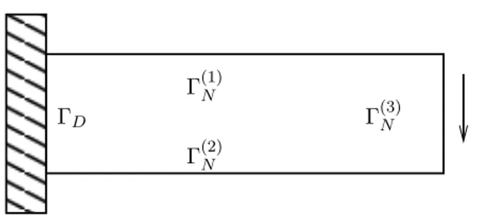
ΓD

Γ(1)_N

Γ(2)_N

Γ(3)_N

1

Figure 6: Illustration of a mixed Dirichlet, Neumann boundary value problem. The external surface forces might, for example, be g = 0 on Γ(1)_N ,Γ(2)_N and g = −e3 on

Γ(3)_N . (In that case we would say that Γ(1)_N and Γ(2)_N are free.) The Dirichlet boundary condition would be imposed in the form y(x) = yD(x) =x on ΓD.

These forms are slightly more general than the examples previously discussed and are sufficient for most applications. (Note: The force f(x) = ˆf(x, y(x)) is the force

per unit volume in the reference configuration, as opposed to b(x) which is the force

per unit mass in the reference configuration. We call ˆf and ˆg the forcing functions.

A forcing function ˆf or ˆg is called a dead load if it depends only on x, but not on the deformation itself. Gravity (in the approximation where one of the bodies (the earth) is much larger) is the prototypical example of a dead load. Dead loads represent primarily a simplification from the mathematical point of view and rarely occur in realistic models.

7.2 The boundary value problem

We will, in later sections, reduce the task of determiningTˆ further. For the time being, we accept the general form (19), satisfying also (20), and turn to the boundary value problem of (nonlinear) elasticity.

Under these conditions, the equations of equilibrium (17) become the pure Neu-mann problem (or, pure traction problem):

−DivTˆ(∇y) = ˆf, in Ω, (21a)

ˆ

T(∇y)N = ˆg, on∂Ω. (21b)

(31)

problem:

−DivTˆ(∇y) = ˆf, in Ω, (22a)

ˆ

T(∇y)N = ˆg, on ΓN, (22b)

y= yD, on ΓD. (22c)

If ΓD =∅, then (22) reduces to (21); if ΓD =∂Ω, then (22) is called thepure Dirichlet

problem.

Other, more complicated situations are also possible. For example, a flat side of a body might be clamped only in thex3 direction. In that case, part of the boundary

has both Dirichlet and Neumann conditions. For simplicity, we do not consider this possibility at the moment.

Example 7.1 (A generic solution). We seek an equilibrium solution of the form

y(x) =F x+c,

where F ∈M3×3

+ and x∈R3 are constants. In that casex7→Tˆ(∇y) is constant and

hence (22a) is automatically satisfied. If we consider a pure Dirichlet problem with

yD(x) =F x+c, then y(x) is a solution of (22).

Example 7.2 (Physical examples of non-uniqueness). The classic notion of well-posedness of a boundary value problem such as (22) is existenceand unique-ness of solutions (understood in an appropriate sense). The question of existence is particularly difficult and goes deep into the theory of partial differential equations and the calculus of variations (see for example [Cia88, Ch. 6, 7]). This is well beyond the scope of this course. What we can study at a fairly informal level is the question of uniqueness. In the following we will discuss four simple example that demonstrate conclusively that we cannot expect unique solutions to the equilibrium system (22). The letters in the following list correspond to the letters in Figure

(a) Torsion of a cylinder: Consider a cylinder of a very flexible material

(e.g., rubber) in a stress free state. Then this state solves the BVP (22) with no-displacement boundary condition at each end (all external forces are zero). Now keep one end of the cylinder fixed and rotate the other end by 360 degrees. Keeping the end fixed again, we obtain a second solution to the BVP (22) with the same boundary conditions. In principle, this process can be repeated and one can obtain a countable ste of equilibrium solutions.

(b) Buckling of a rod: Consider again a cylinder (or rod) or a very flexible

(32)

1. INTRODUCTION 5

Figure 1.1: Two stable equilibria of an elastic body with the same boundary conditions. Modified from [30, p. 247].

The aim of the present section is to discuss this somewhat controversial postulate. For example, in [90] Tartar states: ‘I like to call ultra-science-fiction elastic materials those. . . inexistent materials which instantaneously discover a minimum of their po-tential energy. . . ’. Tartar’s statement is intended to criticise, first, the fact that the evolution is entirely neglected (cf. [90, p.7], ‘I do not think there is much Physics in a model where there is no time.’ ), and second, that the material is assumed to attain a

globalenergy minimum.

In fact, for many mechanical systems simple counterexamples to the principle of global energy minimiation may be constructed. A well known counterexample from the theory of elasticity is the elastic rod shown in Figure 1.1. If the deformation is held fixed at both ends then the energy minimum is the undeformed state shown at the top of Figure 1.1. If the left-hand end is still held fixed, but the right-hand end is twisted by 360 degrees and then fixed in the same position as before, we obtain a newstable equilibriumunder the same boundary conditions. Since, by allowing the right-hand face to deform freely, the elastic rod would return to its reference state, the twisted deformation must have a higher energy than the undeformed state and is therefore notglobally stable. By iterating the process, it can be seen that the elastic energy has infinitely manystable equilibria.

While, based on these arguments, we may decide not to accept the principle of global energy minimization without a great degree of suspicion, we may still be interested in static equilibria only. It would seem a waste of resources to use dynamics to find a stable equilibrium of the system. Nevertheless, the stability of an equilibrium is inherently related to the evolution equation that is satisfied by the system as well as the perturbations from equilibrium which it is subjected to.

What is meant by a stable equilibrium (or meta-stable state) has to be decided in each particular case. Any general definition such as ‘local energy minima’ (with respect to a specific metric) is unlikely to be sufficiently strong for applications. Throughout

(a) (b)

y(x) =xon∂Ω

Multiple solutions of the equilibrium equations are expected corresponding to rotations of the inner cylinder through integer multiples of 2π. In the figure the image of the dotted line in the reference configuration is shown when the rotation is through 2π.

Other examples of non-uniqueness occur in pure dead-load traction prob-lems. B! Ω A B A! B! C! D! D C A! C! D!

The figure shows a circular cylinder with tangential equal forces applied to its boundary. We expect a deformation as shown in which the dead loads point radially outwards (so thatAmoves toA!_{etc), but also another (unstable) one}

in which the loads point radially inwards.

There are examples for pure zero traction boundary conditions also.

29 (c)

y(x) =xon∂Ω

Multiple solutions of the equilibrium equations are expected corresponding to rotations of the inner cylinder through integer multiples of 2π. In the figure the image of the dotted line in the reference configuration is shown when the rotation is through 2π.

Other examples of non-uniqueness occur in pure dead-load traction prob-lems. B! Ω A B A! B! C! D! D C A! C! D!

The figure shows a circular cylinder with tangential equal forces applied to its boundary. We expect a deformation as shown in which the dead loads point radially outwards (so thatAmoves toA!_{etc), but also another (unstable) one} in which the loads point radially inwards.

There are examples for pure zero traction boundary conditions also.

29

(d)

Figure 7: Several physical examples of nonuniqueness in the boundary value problem of elasticity (22); cf. Example 7.2.

(c) Pure Neumann problem. In example (c), we apply surface forces in a way

so that two equlibria exist. If we turn the reference configuration clockwise in the direction of the forces, then we end up in a stable equilibrium (whereC0_{is left and}_A0 is right). If we turn the reference configuration counterclockwise against the direction of the forces, then we end up in an unstable equilibrium (with A0 _{on the left and}

C0 _{on the right). This problem can be understood either as a 2D example or as an} axisymmetric 3D example.

(d) Pure Dirichlet problem. Next, we consider a pure Dirichlet problem, which

is easiest to discuss in 2D. By fixing the inner edge and rotating the outer edge of the annulus by 360 degress, then fixing the body in that position, we end up with an equilibrium that satisfies the pure Dirichlet condition y(x) = xon ∂Ω. A similar 3D example is quickly constructed, for example, by deforming a thick shell in a similar way.

(e) Zero traction problem. The final example is not contained in Figure 7. If

we take a thick rubber sphere (for example, a tennis ball) and cut a sufficiently large hole in it, then we can push the ball through the hole (i.e., evert it). This new state

(33)

7.3 Hyperelasticity and conservative forces

A homogeneous elastic material is called hyperelastic if there exists a stored energy

function (or, strain energy density) W :M3×3

+ →Rsuch that

ˆ

T(F) = DW(F) ∀F ∈M3×3

+ . (23)

If a material is hyperelastic, then it can be easily shown that the total work done by external forces in a closed quasistatic process is zero. A map y: Ω×(t1, t2)→R3

is called a motion if it is “smooth” (at least C1 _{in both variables) and} _y_(·_{, t}_{) is a}

deformation for each fixed t. The motion is called a quasistatic process if y(·, t) is in static equilibrium for some external forces ˆf,gˆthat may now also depend on t.

The work done by the external forces on a part E of the body is

work[y;E] =

Z _t₂

t1 ( Z

∂E(TN)·∂tydA +

Z

E(bρ)·∂tydV

)

dt.

Integration by parts (the divergence theorem) gives

work[y;E] =

Z _t2

t1 ( Z

E DivT+bρ

·∂tydV +

Z

ET:∂tF dV

)

dt

=

Z _t₂

t1 Z

E

ˆ

T(F) :∂tF dV dt

=

Z _t2

t1 ∂t

Z

EW(F) dV dt.

Hence, ifyis aclosedprocess (i.e.,y(·, t1) = y(·, t2)) then the work is zero. Employing

standard ideas of calculus, it can be seen that this condition is also sufficient. In fact, we have the following stronger result:

Theorem 7.3. A material is hyperelastic if and only ifwork[y; Ω] ≥0for all closed

quasistatic processes y.

Sketch of the proof. We have shown above that hyperelasticity is sufficient that the

total work is zero. Thus, it only remains to show that, if the work is non-negative then (23) holds.

A complete proof of this statement is slightly complex, but the main ideas can be quickly sketched out. What we will ignore in this sketch are a few somewhat subtle smoothness requirements on the paths that we use.

Step 1.To begin with, we concentrate only on trajectories of homogeneous

defor-mations, i.e.,∇xy(x, t) =F(t). In that case, bρ= 0, and we simply obtain

Z ₁

0 Z

∂Ω(

ˆ

(34)

F

F(t)

(F+εH)(t)

F+tεH

F+εH M3+×3

1

Figure 8: Cartoon of step 3 in the proof of Theorem 7.3.

Integrating by parts gives us

Z

∂Ω(

ˆ

T(F)N)·∂tydA =

Z

Ω

ˆ

T(F) : ˙F dV =|Ω|Tˆ(F) : ˙F ,

that is, _Z

1

0

ˆ

T(F) : ˙F dt≥0

for all closed trajectories F(t) in M3×3 + .

Step 2: work = 0.LetF(t) be a closed trajectory inM3×3

+ , then the time-reversed

trajectory F∗₍_t_{) =}_F₍₁₋_t_{) is also closed and hence}

0≤

Z ₁

0

ˆ

T(F∗_{) ˙}_F∗_d_t ₌₋Z 1 0

ˆ

T(F(1−t))( ˙F)(1−t) dt =

Z ₁

0

ˆ

T(F(τ)) ˙F(τ) dτ.

Thus, we have shown that _Z

1

0

ˆ

T(F) ˙F dt= 0

for all closed trajectories F(t) in M3×3 + .

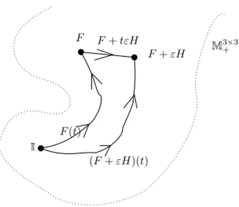
Step 3. The final step in the proof is a standard argument from calculus, and we

will therefore be brief. Since M3×3

+ is connected, we can take a path (F(t))t∈[0,1] from

any arbitrary fixed matrix, say, 1 to F and define

W(F) =

Z ₁

0

ˆ

T(F(t)) ˙F(t) dt.

The main point here is that, due to step 2, this integral is independent of the path chosen.

LetH ∈M3×3 _{and let}_ε_{be sufficiently small so that}_F₊_tεH _∈_M3×3

+ fort∈[0,1].

(35)

Figure 8)

W(F +εH)−W(F) =

Z ₁

0

ˆ

T(F +tεH) : (εH) dt.

Dividing by ε and letting ε→0, we obtain

DW(F) :H =Tˆ(F) :H ∀H ∈M3×3_.

This concludes the (sketch of the) proof.

We will assume from now on that the material is hyperelastic, i.e., that the stress-strain relation satisfies (23).

An interpretation of W can be obtained as follows: the functional

Eel(y) := Z

ΩW(∇y) dV

is the elastic energy stored by the body under the deformation y. With this interpretation in mind, it is reasonable to assume that

W(F)→+∞ as detF →0+, (24)

so that infinite energy is required to compress a body to zero volume.

7.3.1 Conservative forces

An applied body force is said to be conservative if there exists a potential φb :

Ω×R3 _→ _R _(the _{potential of the applied body force}_{), differentiable in the second}

component, such that ˆ

f(x, y) =Dyφb(x, y) ∀x∈Ω ∀y∈R3.

A similar definition can be made for the surface force ˆg if it only depends on

x, y but not on ∇y. However, the∇y-dependence is required in important cases (cf. Example 6.5), and these require a more general treatment (cf. Example 7.2).

All dead loads are conservative and the associated potentials are

φb(x, y) = ˆf(x)·y and φs(x, y) = ˆg(x)·y.

7.3.2 The variational problem

The following principle will also work in the case of conservative applied forces, but for the sake of simplicity, we assume that all forces are dead loads. In that case, we can define the total energy

I(y) =

Z

Ω

W(∇y)−fˆ·ydV−

Z

ΓN ˆ