(will be inserted by the editor)
Dynamic collective bargaining and labor adjustment
costs
Francisco Cabo · Angel Mart´ın-Rom´an
the date of receipt and acceptance should be inserted later
Dynamic collective bargaining and labor adjustment costs
Abstract Collective bargaining between a trade union and a firm is analyzed within the framework of a monopoly union model as a dynamic Stackelberg game. Adjustment costs for the firm are comprised of the standard symmet-ric convex costs plus a wage-dependent element. Indeed, hiring costs can turn into benefits assuming wage discrimination against new entrants. The union also bears increasing marginal costs in the number of layoff workers and de-creasing marginal benefits in the number of new entrants. Starting from a baseline scenario with instantaneous adjustment, we characterize the condi-tions under which the adjustment costs for the firm, or for the union, lead to higher employment and lower wages or vice versa. More generally, these adjustment costs, when they affect both the union and the firm, are generally detrimental to employment. However, the standard symmetric element of the adjustment costs for the firm positively affects employment, even with lower wages. Finally, if hiring and firing costs are defined separately, then hiring and firing could take place simultaneously if the wage discrimination towards new entrants is strong, because the firm would agree to pay the costs of firing incumbent employees, in order to enjoy wage savings from new entrants.
JEL Codes: J5, J23, C73, C61.
Keywords: Dynamic labor demand, collective wage bargaining, monopoly union model, adjustment costs, Stackelberg differential game.
Francisco Cabo
IMUVa, Universidad de Valladolid, Spain. E-mail: [email protected]
Angel Mart´ın-Rom´an
1 Introduction
The process of collective bargaining between a representative firm and a trade union is analyzed from a dynamic perspective. In a dynamic labor market, our attention is centered on the progressive expansion or contraction of the set of workers employed within the firm and the evolution of the wage they earn. The dynamic aspects of the interaction between the firm and the union are based on the existence of adjustment costs, that is, on how the firm’s profits and the union’s welfare are affected when new employees are hired or existing workers are fired. We use the termadjustment costsin concordance with the literature. However, these costs will be positive when firing occurs but will be typically negative when hiring occurs. Adjustment costs are crucial in determining the speed of convergence, as well as determining the steady-state equilibrium of both employment and wages.
We introduce two considerations which drive the dynamics of the collec-tive bargaining process and which, to the best of our knowledge, have not been previously addressed by the literature. First, on the firm’s side, the con-ventional adjustment costs, exclusively dependent on the number of hired or fired employees, are extended by assuming that these costs also depend on the prevailing wage. Thus, we define a two-part adjustment cost for the firm. Second, we also assume that the entrance of new employees and the layoff of current employees also affect the union’s welfare and its behavior. We model a full-coverage industrial relations system in which all workers are affected by the union’s decisions about wage.1Thus, workers benefit from the union’s achievements regardless of whether they are members or not. Or put differ-ently, the union represents members and non-members identically. These are habitual industrial/labor relations in some countries in Continental Europe.2 The model developed in this paper could be included within the insider-outsider literature from a broad perspective. Some previous works model col-lective bargaining within an insider-outsider theoretical setting from a static standpoint. An excellent example of this literature is Holden (1990). Our work, on the other hand, contributes to the dynamic insider-outsider literature which can be dated back to Solow (1985), and which has produced interesting theo-retical models such as Drazen and Gottfries (1990), Huizinga and Schiantarelli (1992), Fukuda and Owen (2008) and, more recently, Gal´ı (2016), for example. The four central assumptions on which an insider-outsider model rests, (Lind-beck and Snower 2001) are fulfilled: “(1) Firms face labor turnover costs that they cannot entirely pass on to their employees. (2) Insiders have some market
1 The notion of a union’s “influence” nowadays seems to be more important than a union’s “presence” (see Boeri and VanOurs, 2013 p.64). The concept of “excess coverage” (i.e. col-lective bargaining coverage rate minus union density rate) appears to be central to under-standing industrial and labor relations currently. A proof of this statement is that coverage is usually higher (specially relevant in cases like France, Austria or Spain) than union density in most of the countries (Boeri and VanOurs, 2013 p.65).
2 For instance, Cahuc et al. (2014, p. 404) point out: “(. . . ) in France and Spain collective
power. (3) If entrants remain with a firm long enough, they become associated with the same labor turnover costs as the insiders, and have an opportunity to renegotiate their wage. (4) Employment decisions are made unilaterally by the firms.” The bargaining process presented in this work shares these four main characteristics of insider-outsider models and seeks to describe the functioning of several European labor markets with large rates of union coverage.
In summary, in this paper we model the bargaining process between a trade union and a representative firm in a dynamic labor market. The dynamics stem from the adjustment costs for the firm and the trade union associated with hiring and firing decisions. The equilibrium concept considered in the paper is a partial steady-state equilibrium in which aggregate supply-side forces (i.e. labor supply and labor demand interactions) drive the allocations of wages and employment.3
The rest of the paper is organized as follows: The second section discusses and introduces, in an informal way, the adjustment costs for the firm and the union that we claim play an important role in the bargaining process, and places them within the existing literature on collective bargaining. The formal model is built in the third section. The fourth section analyzes the baseline scenario with instantaneous adjustment, and two intermediate scenarios with adjustment costs only for the union or only for the firm. The general Stackel-berg game with adjustment costs for both players is solved in the fifth section, which also presents a sensitivity analysis of the main parameters describing these costs. The sixth section presents a broader approach in which hiring and firing decisions are taken separately, which opens up the possibility that hiring and firing occur simultaneously. Conclusions are presented in the seventh and final section.
2 Adjustment costs for the firms and the union
2.1 Dynamic labor demand
The literature on dynamic labor demand has frequently considered symmetric adjustment costs in hiring and firing.4These adjustment costs are usually rep-resented by a strictly convex function, or sometimes a piecewise linear function in hiring and firing (see, for example, Nickell 1987). This formulation does not distinguish between hiring and firing costs, even though the empirical liter-ature has frequently stressed that these differences do exist. It is generally admitted that hiring costs are higher than firing costs in countries like the United States (see Hamermesh 1996, for a review of some studies), whereas
3 We analyze the steady-state equilibria, although considering the capital stock as an exogenous constant. Thus, only the employment level adjusts, and not the capital stock and therefore we do not characterize a long-run equilibrium.
the opposite is true for continental Europe (e.g. Abowd and Kramarz 2003; Goux et al. 2001, for French data).
For this reason, some authors departed from the assumption of symmet-ric quadratic adjustment costs in the late 1980s and early 1990s, introduc-ing asymmetries (two excellent surveys on this literature are Hamermesh and Pfann 1996 and, more recently, Hamermesh 2017). Within the category of convex yet asymmetric costs, we can highlight Pfann and Palm (1993), Chang and Stefanou (1988), and Jaramillo et al. (1993). Some authors consider a piecewise linear specification of the adjustment cost for labor, with a constant marginal cost which diverges between hiring and firing (see the seminal works by Bentolila and Bertola 1990, Bertola 1990, Bentolila and Saint-Paul 1994, and Bertola and Rogerson 1997). Finally, some authors have addressed the existence of lump-sum costs, such as the search costs for certain categories of personnel (hiring), or the administrative costs of collective dismissals in many European countries (firing). These costs are independent, to a certain extent, of the number of employees hired or laid off. These fixed costs explain why, under certain circumstances, firms have an interest in hiring and firing in groups. Some representative works of this strand of literature are Hamermesh (1995), Abowd and Kramarz (2003), Hall (2004), Varej˜ao and Portugal (2007) and Kramarz and Michaud (2010).
Within the context of asymmetric labor adjustment costs, we focus on the case in which firing costs are more important than hiring costs. This is typically the case in continental Europe and particularly in Southern Europe.5Although hiring is associated with costs like recruiting and training, it also represents an opportunity for wage savings, if new entrants are paid a lower wage than senior workers. Newly-hired workers (whom the union is less concerned about) are outsiders and for that reason receive an initial lower wage while they become insiders.6 The net effect of hiring on the firm’s accounts would depend on the relative size of the hiring costs versus the wage savings from the salary gap of new entrants. The first term exclusively depends on the number of hired workers, while the second is also crucially dependent on the prevailing wage: if the wage discount to new entrants is a fix percentage of the prevailing wage, then the greater this wage, the greater the wage savings from hiring.
On the other hand, the firing costs clearly grow with the number of fired employees. Moreover, we additionally assume a positive relationship with wages,
5 Cahuc et al. (2014, p.120) stated that: “(...) in countries where strong legal measures
are in place to enhance job security, the costs of separation outstrip recruitment costs”.A well-documented example of this empirical regularity is France (Abowd and Kramarz 2003; Goux et al. 2001). This is also true for other Southern European countries. Boeri and van Ours (2013, p. 278) shows how France (3.0), Greece (3.0), Portugal (3.2), Italy (2.6), and Spain (3.1) exhibit extremely high levels in the overall employment protection legislation index. By contrast, English-speaking countries like Australia (1.4), Canada (1.0), Ireland (1.4), New Zealand (1.2), the United Kingdom (1.1), and the United States (0.9) tend to show the lowest levels for this index.
as legislation in many countries typically links severance packages to the wages of the laid off workers.
Thus, the adjustment costs of hiring and firing are defined in two parts. A first part, exclusively dependent on the number of hired or fired employees, collects the standard assumption of symmetric convex costs. The second part is a wage-dependent component that increases firing costs but conversely reduces hiring costs, indeed turning hiring costs into net benefits. It is due to this component that the adjustment costs are asymmetric.
Finally, we formulate the hypothesis that countries with higher firing costs (in weeks of wages) also show a wider salary gap. This assumption is made for tractability, although it is not far from the reality as shown by empirical data in Dias da Silva and Turrini (2015). These authors point out that there is a direct relationship between the cost of firing (measured through various dimensions of the employment protection legislation index) and the permanent versus temporary wage gap across countries. The justification for this relies on the different bargaining power of workers with an open-ended contract versus those with a fixed-term contract. In other words, stronger employment protection for the permanent workers allows them, at the same time, to obtain a higher wage differential with respect to their temporary counterparts. If we consider that the newcomers are typically hired with a fixed-term contract, the previous argument and the empirical evidence attached to it give credit to our hypothesis. This hypothesis will be relaxed in the sixth section, allowing for differences between the marginal firing costs and the wage gap of new entrants.
2.2 Dynamic collective bargaining
The dynamic interaction between the firm and the union7 can be studied by introducing the adjustment costs of hiring and firing for the firm into the collective bargaining process. A pioneer work in this literature is Lockwood and Manning (1989), who analyze a dynamic model that takes into account quadratic adjustment costs for the firm in a discrete setting and considers a right-to-manage framework. The wage is jointly settled by the firm and the trade union (according to their bargaining power), and then the firm unilater-ally determines employment. In this setting, convergence to the steady state is faster than in the competitive equilibrium case. This type of adjustment costs is also studied by Modesto and Tomas (2001) within the framework of a monopoly union model, in which the firm chooses the optimal employment level, and the union determines the optimal wage rate knowing the labor
mand fixed by the firm. The non-cooperative equilibrium is confronted with the equilibrium under the cooperative or dynamically efficient bargaining model.8
Alternatively, dynamics can be introduced by assuming that employment follows a stock adjustment principle, where an “exogenous” constant fraction of the gap between the desired and the actual number of workers is closed at each instant of time. This was first explored in Booth and Schiantarelli (1987) for a monopoly union model. However, the most fruitful strand of research from a dynamic perspective has been the analysis of union membership. Two influ-ential papers in this literature are Kidd and Oswald (1987) and Jones (1987), who consider endogenous membership and analyze a monopolistic trade union that cares about current and future members. The hiring decisions of the firm have an effect on the union, under the assumption of full-coverage, or alterna-tively, if new recruits immediately join the union. Correspondingly, the layoff of current employees induces welfare losses to the union.9
The analysis of union membership is relevant when members have privi-leges over non-members. The union membership models usually capture some stylized facts of the industrial relations systems of English-speaking countries. As already pointed out, in France and Spain practically all workers are cov-ered under a collective bargaining agreement, independently of whether they are union members or not. Moreover, in Nordic countries (and more gener-ally in those countries under the Ghent system) the incentives to become a union member are rather different from those described in the canonical union membership model. Under the assumption of full-coverage, the union nego-tiates on behalf of all employees (members or not members). In this setting, the relevant distinction is not between members and non-members, but be-tween incumbents and new entrants. The union focuses mainly on incumbent or insider privileged employees,10while outsider workers will face less favorable employment conditions when hired (in particular, an initial lower wage). Thus, we deviate from the literature on union membership. By contrast, the dynamic aspect associated with the union will be the existence of firing disutilities and hiring benefits also.
Next, we describe the adjustment costs for the union. It is assumed that firings reduce the union’s welfare at an increasing rate. This is corroborated by the strong opposition of the trade unions to reductions of large numbers of employees at once, but much softer resistance when firings occur gradually and are restricted to a few employees. Correspondingly, the union welcomes the
re-8 Both the right-to-manage model and the monopoly union model are studied in Koba (2003), who analyzes the effect of deregulation on employment and wages.
9 Some interesting works in this strand of research are Chang and Lai (1997) and, more recently, Dittrich and Schirwitz (2011a), Dittrich and Schirwitz (2011b), or Kazanas and Miaouli (2014).
cruitment of new employees, although at a decreasing rate.11This assumption can be based on organizational aspects; the arrival of new employees can give rise to a number of problems such as managerial problems in the union. Like-wise, we could also resort to the Agency Theory that considers the union as the agent and the collective of workers as the principal, (see Faith and Reid, 1987). Under this view, hiring enhances the union’s utility at a decreasing rate due to the organizational problems for the agent. Indeed, if the hiring rate becomes disproportionately high, congestion problems might make fur-ther hirings unattractive. This decay in the marginal hiring gains would be amplified if the principal was composed of the insiders (in an insider-outsider framework). Then, the gains for the principal would also decrease with the number of new entrants, who could, for example, threaten their future social status. This specification of the adjustment costs indicates that the union is strongly concerned about current employees (insiders), whose dismissal would reduce the union’s welfare, but is also partially worried about unemployed workers (outsiders) as they would be welcomed if hired.
The aim of the paper is to analyze a partial equilibrium focusing on the supply-side forces that drive the allocations of wages and employment. We do not analyze long-run aspects like the process of investment and capital accumulation. A seminal work in this literature is van der Ploeg (1987), who studies the implication of long-term wage contract for a neoclassical firm. More recently Chang et al. (2007) studies the effect on endogenous growth of the internal conflicts faced by a political trade union.
3 The two actors in the collective bargaining process
Collective bargaining in a monopoly union model involves two agents: a firm, which acts as the follower, and a monopolistic trade union, which takes the role of the leader. The former has to determine the recruitment of new employees (or the layoff of current employees) at each instant of time. The latter, given its monopolistic role, determines wages optimally, knowing the firm’s demand for new employees.
Employment, L(t), is not considered as a decision variable but as a stock variable. Therefore, the level of employment at time t, can be defined as the initial stock of workers within the firm,L0, plus the accumulated flow of em-ployees recruited and not fired, and minus the accumulated flow of emem-ployees who voluntarily quit the firm from the start and up to the current time:
L(t) =L0+
Z t
0
h(τ)dτ−
Z t
0
δL(τ)dτ, L0≥0,
with δ >0 being the voluntary quit rate, assumed constant for tractability. The flow variable, h(t), can be positive, implying new recruits, or negative,
representing firings. Meanwhile, employment should not take a negative value,
L(t) ≥ 0. The evolution of employment can be alternatively defined by the differential equation:
˙
L(t) =h(t)−δL(t), L(0) =L0≥0. (1)
According to this specification, the firm optimally adjusts the level of employ-ment.
3.1 The employer
The main interest of this paper is to analyze to what extent the adjustment effects or frictions in the labor market can affect the employment level and the wage rate at the equilibrium, and the speed of convergence towards this equilibrium. The installed capital stock is taken as a given constant, hence production is only dependent on the total amount of labor Y(L(t)), charac-terized by a labor productivity which decreases in the employment level. For tractability, the specification considered here is a linear quadratic function in the level of employment,L(t):
Y(L(t)) =aL(t)−L 2(t)
2 , L(t)∈[0, a],
12 (2)
with a > 0 the highest possible labor productivity (attained for L(t) = 0). This parameter collects, among other factors, the installed capital stock and the level of technology, both assumed to be time-invariant.
Under the unit price hypothesis, with no adjustment costs of hiring or firing, the profits of the firm would be defined as total output minus the wage bill paid to employees,Y(L(t))−w(t)L(t), withw(t) the identical wage rate for all employees regardless of their seniority. The firm’s finances are also affected by the frictions from the hiring or firing of employees. Hence, the firm cannot bring forth the desired employment level instantaneously and at no cost, but must develop it gradually. Focusing on hiring, denoted by
h+(t) ≥ 0, the adjustment costs are defined as the addition of two terms. First, the standard convex adjustment costs,13 AC(h+), (AC0(h+) >0 and
AC00(h+)≥0)14, which encompasses the cost of advertising and interviewing plus the training cost. Additionally, a second term considers the dependence on the prevailing wage. Total employees at any point in time can be divided between the insiders, or incumbent employees, and the new entrants,h+. New entrants face less favorable working conditions, reflected by a salary,wn, below the wage obtained by insiders,w. The wage savings define the second part of
12 A level of employment aboveais not feasible as it would imply lower output and higher labor costs.
13 This standard assumption is not exempt from criticism. Nickell (1987) states that for low levels of hiring it is hard to think of good reasons why hiring costs should increase at the margin.
the adjustment costs from hiring: (w−wn)h+, which actually represents a profit or a negative adjustment cost for the firm.
If, conversely, we focus on firing, denoted byh−≥0, the adjustment costs are again defined by the same standard convex adjustment costs, AC(h−), plus a second term dependent on the wage rate. This term is defined as a percentage,β, of the current wage times the number of fired employees, and it is based on the fact that the severance package paid to layoff employees, in many countries, is defined as a percentage of their wage at work.
Furthermore, we also assume that the wage gap remains constant in relative terms and indeed equal toβ: (w(t)−wn(t))/w(t) =β∈(0,1). This assumption implies that a higher wage increases the marginal costs of firing by the same amount as the marginal profits from hiring.15 Under these assumptions, it is possible to merge hiring and firing decisions in a single variable,h, which takes a positive value when the firm hires employees, and a negative value when it fires current workers. Thus, the adjustment cost from hiring,AC(h+)−(w−
wn)h+, or firingAC(h−)+βwh−can both be represented by the same function:
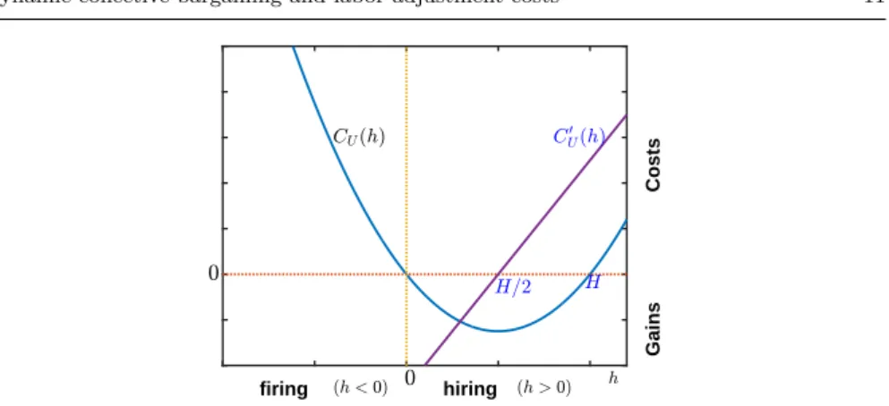
CF(h, w) =c h2
2 −βwh, c, β >0, (3)
where a quadratic specification for the standard convex costs, AC(h), is as-sumed. This representation implicitly assumes that the firm either hires or fires employees (h+ and h− can not be strictly positive at the same time). From expression (3) it follows that hiring h+ > 0 and firing h− > 0 would imply adjustment costs ofCF(h
+, w) +C
F(−h
−, w). By contrast, hiring a net amount ofh+−h−(or firing if negative) is associated with adjustment costs of
CF(h+−h−, w). From expression (3), it follows thatCF(h+, w)+CF(−h−, w)> CF(|h+−h−|, w). As a result, our assumption that hiring and firing cannot
occur simultaneously holds for the specification in (3).
Moreover, notice that expression (3) does not imply symmetric hiring and firing costs, unless β = 0. As Figure 3.1 shows, the wage-dependent term increases the adjustment costs when firing, but decreases these costs when hiring. In fact, a firm which hires workers enjoys net gains if the number of new recruits is not too large. For hiring rates below the upper bound, 2βw/c, wage savings from new entrants more than offset standard hiring costs. It is worth noticing that, at the steady-state equilibrium, the firm necessarily ends up hiring exactly the fraction of employees that quit voluntarily. Because of that, from the double interpretation ofβ, what matters at the equilibrium is its role as a measure of the wage discrimination or wage gap between incumbent employees and newcomers. The interpretation of β as the wage-dependent part of the firing costs may be relevant for short-term adjustment, under an initial situation of excessive employment, at which the firm has to fire some workers within an initial finite period. However, this interpretation is only valid temporally because, even in that situation, firings will stop at some point and,
h
hiring (h >0)
firing (h <0) 0
0
CF(h)
AC(h) ch
2
2!-wh
Costs
Gains
Fig. 1 Adjustment costs for the firm
as the steady state approaches, the firm hires workers to replace those who voluntarily quit.
The profits of the firm are defined by the income from production, Y(L), minus the wage bill and the adjustment costs associated with hiring and firing:
WF(h, w, L) =Y(L)−wL−CF(h, w),
with the production function given in (2) and the adjustment costs in (3).
3.2 The trade union
Under the assumption of full coverage, the union represents all laborers (em-ployed or unem(em-ployed). Taking into account an expected utility approach and normalizing the total population to one, the instantaneous union’s utility reads: WU(w, L) = Lu(w) + (1−L)u(B), with B the unemployment
bene-fit, andu(·) a concave utility function. Thus, the union is concerned about the excess utility from the insiders wage above the unemployment benefit as well as the utility of unemployed workers. Moreover, it is also affected by the hiring and firing decisions of the firm. This subsection describes how the (positive) adjustment costs of firing and the (negative) adjustment costs of hiring affect the union’s objective function.
h
hiring (h >0)
firing (h <0) 0 0
CU(h) CU0(h)
H=2 H
Costs
Gains
Fig. 2 Adjustment costs for the union
or organizational problem for the union can be more clearly seen considering a principal-agent problem, with the union as the agent and the insider employees as the principal.
The hypotheses of increasing marginal costs from firing and decreasing marginal gains from hiring can both be encompassed by a single function describing the adjustment costs of hiring and firing for the union:
CU(h) =d
h(h−H)
2 , d >0, (4)
wheredmeasures the relative importance of the adjustment costs with respect to the utilitarian part of the union’s welfare. This linear-quadratic function al-lows analytical tractability and satisfies the fundamental requirement that the marginal gains from new entrants decrease with the number of hired employ-ees. Moreover, as depicted in Figure 3.2, when hsurpasses H/2 hiring stops being attractive for the union, i.e.C0
U(h) becomes negative, and an additional
employee is no longer welcome. We believe that this implication is not unreal-istic, based on organizational problems for the union. Nonetheless, given that the population has been normalized to one, this possibility could be easily dropped by assumingH ≥2.
Finally, adding the adjustment cost to the union’s welfare and assuming risk-neutral laborers (i.e. a one-to-one utility function), the objective function for the union would read
WU(h, w, L) =Lw+ (1−L)B−CU(h).
4 The role of adjustment costs on collective bargaining
this section characterizes the labor market equilibrium in successive stages. In the first stage we obtain the wage and the employment level when neither firm’s profits nor union’s welfare are influenced by hiring or firing decisions. With no adjustment costs associated with hiring or firing the stock of employees (and correspondingly the wage) adapts instantaneously, and hence, the collective bargaining is a simple static monopoly union model. In a second stage, we introduce the adjustment costs only for one of the players, the firm or the union. In either case interaction becomes a dynamic process and employment progressively adapts to its steady-state value. By comparing the steady-state equilibrium for these models to the equilibrium with instantaneous adjustment, it is possible to follow the trail of how the wage and the level of employment are affected by the adjustment costs faced by either the firm or the union. In the last stage, the final subsection analyzes the differential game when the firm and the union are both affected by adjustment costs associated with hiring and firing.
4.1 A game with no adjustment costs
With no adjustment costs and no restriction on the number of hired or fired employees, the firm can instantaneously adapt the current level of employment to its desired level. This is a purely static model, presented here for the purpose of contrasting it with the dynamic solutions.
The firm would choose the level of employment to solve:
max
L {Y(L)−wL},
and would replace indefinitely, at no cost, the δLemployees who voluntarily quit. As a result, the optimization problem without adjustment costs is equiv-alent to a static maximization problem. The firm would fix the optimal level of employment at which labor productivity equates wages,Y0(L) =w, which defines the static labor demand,16Lˆs(w) =a−w. Likewise, the monopolistic union faces no adjustment cost and hence, knowing the static labor demand, settles the optimal wage to maximize:
max w
n
wLˆs(w) + (1−Lˆs(w))Bo≡max
w {w(a−w) + (1−a+w)B}.
The wage and the employment level at this static equilibrium are
ws=a+B
2 , L
s=a−B
2 (5)
The wage,ws, can be understood as a convex combination (the mean value) be-tween the maximum labor productivity,a, and the unemployment benefit,B.
That is, between the maximum and the minimum possible competitive wages. The employment level at the equilibrium, Ls, depends on the gap between these two wages. And likewise, it is a convex combination between the zero de-mand at the maximum wage,a, and the maximum demand,a−B, that would occur at the lowest possible wage, B. Since we have normalized total popu-lation to one, the equilibrium is feasible only under condition a∈[B,2 +B], assumed henceforth. In this static setting, the outcome is that a higher labor productivity,a, would increase wages and employment, while a more generous unemployment benefit would raise wages and reduce employment.
4.2 A game with adjustment costs only for the union (c=β = 0)
Facing no adjustment costs, the firm would determine the level of employment by again equating the marginal productivity of labor to wages, hence setting the labor demand function17 LˆAU(w) =a−w. By contrast, in this subsection
firing costs and hiring gains come into the union’s welfare. Given this demand function, it is clear for a monopoly union that changes in wages will be trans-formed into opposite changes in employment levels: ˙w =−L˙. This equation, together with the employment dynamics in (1), allows us to define the dynamic problem for the monopoly union considering the wage as a state variable and replacing the level of employment by the known labor demand function:
max h
Z ∞
0
w(a−w) + (1−a+w)B−dhh−H
2
e−ρtdt,
s.t.: ˙w=δa−h−δw, w(0) =a−L0.
This optimal control problem has a unique solution:18
LAU(t) = (L
0−L¯AU)eφ
AUt
+ ¯LAU, L¯AU =a−B+d(ρ+δ)
H 2 2 +dδ(ρ+δ) ,
wAU(t) =a−LAU(t), w¯AU =a+B+d(ρ+δ)
aδ−H 2
2 +dδ(ρ+δ) ,
hAU(t) =δL¯AU+ (δ+φAU)(L
0−L¯AU)eφ
AUt
, ¯hAU=δL¯AU.
which converges towards the steady-state equilibrium at the speed|φAU|, with
φAU= 1
2
(
ρ−
r
(ρ+ 2δ)2+8
d
)
<0.
By comparing this steady-state with the equilibrium in the scenario with instantaneous adjustment, we observe that:
¯
LAU
RLs⇔w¯AU
Qws⇔hs≡δa−B
2 Q
H
2. (6)
From expression (6) it becomes immediately clear that the existence of ad-justment costs for the union does not necessarily lead to greater wages and unemployment rates. This would be the case only if the size of these adjust-ment costs as measured by H/2 (the range of h compatible with marginal gains from hirings), is small enough in comparison with the voluntary quit rate with no adjustment costs,19hs≡δLs. Therefore, a monopoly union that welcomes the entrance of new employees might fix a lower wage, thereby in-ducing a higher level of employment, and hence a higher voluntary quit rate, than a union only concerned about excess utility if i) the range of newly hired employees that raises union’s welfare, H, is large; ii) the salary gap between the maximum feasible wage and the unemployment benefit,a−B, is small; or iii) the voluntary quit rate is low. Conversely, if these conditions are not met, wages and unemployment would be higher.
4.3 A game with adjustment costs only for the firm (d= 0)
In a monopoly union model, if the firm, which acts as the follower, faces adjustment costs, it would hire in order to solve the dynamic problem:
max h
Z ∞
0
[Y(L)−wL−CF(h, w)]e
−ρtdt, (7)
s.t.: ˙L=h−δL, L(0) =L0≥0. (8)
Given the quadratic structure of the optimization problem, a linear-quadratic value function is conjectured20 VAF
F (L) = a AF F L
2/2 +bAF F L+c
AF F ,
with aAF F , b
AF F and c
AF
F the unknowns to be determined. The firm would fix
recruits up to the point when the marginal effect of an additional employee being hired or fired equates the marginal value of this additional employee for the firm, (VAF
F )
0(L). This optimality condition determines a hiring/firing function dependent on the wage rate and the employment level:
ˆ
hAF(w, L) =wβ+ (V AF F )
0(L)
c . (9)
Note that the marginal effect of hiring is composed of the standard linear marginal adjustment costs,ch, minus the marginal benefits from the wage dis-count to new entrants, given by the fraction, β, of the incumbents’ wage,w. The greater the wage rate, the greater the wage savings from hiring new em-ployees, and therefore the stronger the firm’s incentive to hire, which explains the positive direct effect of wages on hirings.
19 In general, one might presume that the firm welcomes new entrants no matter how large their number. By assumingH/2>1 we could drop the possibility that the marginal benefit for the union from additional hirings can become negative. Then, the adjustment costs for the union would always lead to lower wages and unemployment rates.
The trade union acts as the leader aware of the firm’s hiring policy in (9). It must determine wages in order to maximize its stream of discounted welfare, which assuming no adjustment costs would read
max w
Z ∞
0
[wL+ (1−L)B]e−ρtdt, (10)
s.t.: ˙L= ˆhAF(w, L)−δL, L(0) =L
0≥0. (11)
This linear optimization problem leads to a bang-bang solution for the union of the form
wAF(L) =
wmax≡a ifL+
β c(V
AF U )
0(L)>0,
w∈[B, a] ifL+β
c(V AF U )
0(L) = 0,
wmin≡B ifL+
β c(V
AF U )
0(L)<0,
(12)
where the marginal value of an additional employee for the union, (VAF U )
0(L), remains to be determined.
We consider here that the minimum possible wage fixed by the union is given by the unemployment benefit,B, and the maximum wage by the max-imum productivity of labor, a. Because the union faces a linear problem we guess a linear value function,VAF
U (L) =b AF U L+c
AF
U . Thus, the marginal value
that the union assigns to employment is an unknown constant (independent of the actual level of employment,L), (VAF
U )
0(L) =bAF U .
Because the union faces a linear state optimization problem, the optimal wage fixed by this player is constant, denoted by ¯w. This constant can refer to the minumum wage,B, (if L(t)<−βbAF
U /c for anyt ≥0), the maximum
wage, a, (ifL(t)>−βbAF
U /c for anyt ≥0), or any constant wage ¯w∈[B, a]
(under a singular ray withL(t) =−βbAF
U /cfor anyt≥0).
21Under a constant optimal wage, ¯w, the analytical solution can be found, with22
aAF F =
c(ρ+ 2δ)−√∆AF
2 <0, ∆
AF=c2(ρ+ 2δ)2+ 4c. (13)
bAF F ( ¯w) =
c(a−w¯) +βaAF F w¯ c(ρ+δ)−aAF
F
, bAF U ( ¯w) =
c( ¯w−B)
c(ρ+δ)−aAF F
>0. (14)
From (8), (9) and the expression of aAF
F , the optimal path of employment
reads:
LAF(t) = (L
0−L¯AF( ¯w))eφ
AFt
+ ¯LAF( ¯w), L¯AF( ¯w) = a−[1−β(ρ+δ)] ¯w
1 +cδ(ρ+δ) , (15)
21 We will show that the former is always true and thuswAF(L) =w
max=afor anyt≥0. See the Appendix for more details.
22 The highly cumbersome expressions forcAF
F ( ¯w) andc AF
U ( ¯w) are not relevant and, hence,
which converges to the steady-state equilibrium at the speed|φAF|, with
φAF= 1
2
(
ρ−
r
(ρ+ 2δ)2+4
c
)
<0.
Given that the marginal value of an additional employee for the union, (VAF
U )
0(L) = bAF
U ( ¯w) is non-negative for any feasible value of ¯w, and that L(t) also remains non-negative for allt≥0 (as one can see from (8) and (9)), then LAF(t) +β(VAF
U )
0(L)/c≥ 0, for all t ≥0. If this expression is positive, then from equation (12), it follows thatwAF(L) =a,∀t≥0 satisfies the
opti-mality conditions. Therefore, this is the solution analyzed here. Conversely, if
LAF(t) +β(VAF U )
0(L)/c= 0 for allt≥0, a singular solution could exist. This solution would requireL(t) = 0 for allt≥0, hence it cannot be efficient and can be ruled out, as explained in the Appendix. In this Appendix we also ex-plain why we drop other possible solutions, with jumps from ¯w=ato ¯w=B
or vice versa.
At wagewAF(L) =a, the employment at the steady-state is given by:
¯
LAF(a) = βa(ρ+δ)
1 +cδ(ρ+δ) >0. (16)
And the optimal hiring and firing decisions is obtained by evaluating the hiring rate in (9), ˆhAF(a, LAF(t)).
For this optimal solution, the present value of the ongoing wages paid to an additional worker hired today (who is not fired) and who can voluntarily quit at a rateδ, is given bya/(ρ+δ). Correspondingly, the instantaneous benefit from the hiring of this additional worker is given by the savings from his/her lower wage,βa. From now on, we assume that current savings from hiring do not exceed the ongoing wage costs (otherwise it would be beneficial to hire unproductive workers), as is stated in the next condition.
Condition 1
β < 1
ρ+δ (17)
Since β ∈ (0,1), if we further make the realistic assumption that ρ+δ <1, then Condition 1 always holds.
Although wages are higher than in the case with no adjustment costs, this does not necessarily lead to lower employment levels. Next, we compare employment levels with and without adjustment costs for the firm.
Proposition 1 If hs ≡ δLs > βws/c then, the introduction of adjustment
costs for the firm implies a higher wage and a lower steady-state employment,
¯
LAF(a)< Ls. The opposite is not necessarily true.
Proof See Appendix
The wage savings from hiring new employees induce a direct effect on hirings which can be positive, ifhs< βws/c, or negativehs> βws/c. However, adjustment costs for the firm also induce an indirect negative net23 effect on hirings due to a higher wage. Under condition hs > βws/c the direct and indirect effects are both negative and, as highlighted in Proposition 1 steady-state employment decreases if adjustment costs for the firm are introduced. However, ifhs< βws/cthe comparison between ¯LAF(a) andLsis unclear.
To have better insight into the effect of the adjustment costs on the equi-librium level of employment, in what follows we focus on parameterc, which defines the relative importance of the standard adjustment cost for the firm, and on parameterβ, which represents both the effect that wages have on the firing costs and, more importantly, the wage savings from new recruits. Here and henceforth, we assume that ρ+δ <1, and hence Condition 1 is satisfied for allβ∈(0,1). From (5) and (15), the equation ¯LAF(a) =Lscan be written
as the affine function:
φ(c) =φ0+φ1c=
a−B
2a +
(a−B)(ρ+δ)δ
2a c,
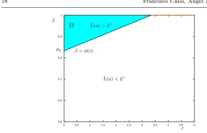
which divides the area [0,+∞]×[0,1] in the cβ-plane into two separated regions at which the existence of adjustment costs for the firm implies a greater ( ¯LAF(a)> Ls) or a lower ( ¯LAF(a)< Ls) employment at the steady state. These regions are depicted in Figure 3, which shows that the adjustment costs for the firm increase employment in region Ω, where the wage savings from new recruits,β, is sufficiently large. This region is nonempty if and only ifφ0<1 provided thatφ1>0.
The area in regionΩcan be interpreted as a measure of the likelihood that the adjustment costs for the firm increase the level of employment. The greater this area, the wider the range of values for parameters β andc at which the existence of adjustment costs for the firm raises employment. This area reads
Ω=
Z ˜c
0
1−φ(c)dc=[B−a(1−2(ρ+δ))] 2
4a(a−B)δ(ρ+δ)2 . (18)
The area in regionΩshrinks with the wage gap between employed and unem-ployed workers,a−B, and widens with the degree of impatience,ρ.
23 A higher wage has a twofold effect on hirings. A positive effect as it represents higher wage savings for the firm. And a negative effect as the marginal valuation of employment by the employer decreases. The partial derivative of ˆhAF(w, L) in (9) w.r.t.wis negative under
0 0.5 1 1.5 2 2.5 3 3.5 4 4.5 5 0.5
0.6 0.7 0.8 0.9 1
-c + L(a)7 > Ls
7 L(a)< Ls -=?(c)
?0
Fig. 3 Comparison ¯LAF(a) vs.Ls
5 A Stackelberg differential game
5.1 A game with adjustment costs for the firm and the union
This section takes into account that firings reduce the firm’s profits and the union’s welfare at an increasing rate. By contrast, new recruits enhance the firm’s profits and the union’s welfare at a decreasing rate.
The monopoly union model analyzed in this section is a Stackelberg dif-ferential game, and the solution concept considered in this dynamic game is the stagewise feedback Stackelberg solution (as it is called in Ba¸sar and Olsder 1982). This type of solution considers a stagewise first-mover advantage for the trade union. Thus, at each time, the union announces the wage to the firm, which then fixes recruitment. Knowing the recruitment decision of the firm for every wage rate, the union determines the optimal wage. For this type of solution, the leader only has an instantaneous first-mover advantage, instead of an inter-temporal advantage as in the global Stackelberg solution. In this latter situation, the decisions made at the start of the game by the individu-als initially running the union should be honored by all future representatives of the union. This can create a credibility problem on the decisions made by the union. By contrast, the stagewise feedback solution is time consistent and therefore credible, with no need of a commitment mechanism.
the corresponding Hamilton-Jacobi-Bellman equation is
ρVF(L) = max
h
aL−L 2
2 −wL−c
h2
2 +βwh+V 0
F(L)(h−δL)
.
From the first order conditions one gets:
VF0(L) =ch−βw
≡ ∂CF ∂h (h, w)
.
The firm hires workers up to the point when the marginal adjustment costs equate to the marginal value of additional employees for the firm. A very large hiring rateh > wβ/ccorresponds to a firm that positively values the entrance of new employees. Conversely, positive firing rates or low hiring rates imply a negative marginal valuation of employees by the firm. Thus, the reaction function for the firm reads
ˆ
h(w, L) =wβ+V 0
F(L)
c , (19)
which is identical to the case where there are adjustment costs only for the firm (as seen in (9)). However, the only differences are the coefficients of the quadratic value function, which can now be defined as24 V
F(L) = aFL
2/2 +
bFL+cF.
Knowing the recruitment policy of the firm, the monopolistic union deter-mines the wage rate in order to maximize:
max w
Z ∞
0
"
wL+ (1−L)B−dˆh(w, L) ˆ
h(w, L)−H
2
#
e−ρtdt,
˙
L= ˆh(w, L)−δL, L(0) =L0.
The Hamilton-Jacobi-Bellman equation for this problem reads
ρVU(L) = max
w
(
wL+ (1−L)B−dˆh(w, L) ˆ
h(w, L)−H
2 +V
0
U(L)(ˆh(w, L)−δL)
)
.
And from the optimality conditions for this problem it must hold that:
L=∂ ˆ
h(w, L)
∂w
h
CU0(ˆh(w, L))−VU0(L)i=β
c
d
ˆ
h(w, L)−H 2
−aUL−bU
. (20)
whereVU(L) =aUL
2/2 +b
UL+cUis the quadratic value function of the union.
A marginal increment in wages increases the wage gains of the collective of employees (at rateL). It also widens the wage gap to new entrants, and hence, the firm’s incentive to hire, ∂ˆh(w, L)/∂w=β/c >0. And more hirings affect the adjustment costs and the marginal valuation of employment by the firm. The optimal wage balances the direct effect of higher wages and the indirect
effect associated with more hirings. From the first order condition (20), and the reaction function for the firm in (19) the feedback strategies for the union and the firm follow:
φw(L) =φ0w+φ 1 wL=
cbU−dbF dβ +
c β
H
2 +
c(βaU+c)−dβaF
dβ2 L, (21)
φh(L) =φ0h+φ 1 hL=
bU d +
H
2 +
βaU+c
βd L. (22)
Note that the optimal recruitment decision of the firm φh(L), paradoxically does not depend on the marginal value of an additional employee for the firm
VF0(L). This occurs because the union settles wages so as to oblige the firm to hire at the rate which balances (20). If the marginal valuation of employment for the firm rises,VF0(L), increasing the firm’s willingness to hire (as shown in (19)), the union will correspondingly reduce wages to lower the wage savings that the firm obtains from new entrants, and hence, to reduce the incentive to hire for the firm. The two effects cancel one another out and hiring and firing decisions of the firm, which is a Stackelberg follower, depend only on the value function of the Stackelberg leader trade union.
Plugging these optimal strategies into the Hamilton-Jacobi-Bellman equa-tions we obtain a system of 6 Riccati equaequa-tions in the unknowns aF, bF, cF, aU, bU, cU. Two sets of solutions for the coefficients of the value functions are
found analytically.25
Proposition 2 A solution for this system of Riccati equations with a concave value function,VU(L), i.e. satisfyingaU <0, is found under Condition 1 and
sufficient condition c≤d(assumed henceforth).
Proof See Appendix
Although no condition is found to characterize the sign ofaF, the numerical
simulations26carried out for different parameters’ values support the hypoth-esis of a positive coefficientaF.
Proposition 3 Under Condition 1, and sufficient condition c≤d,φ0h(L) =
φ1
h<0. Furthermore, ifaF>0(numerically shown) then φ 0
w(L) =φ1w<0.
Proof See Appendix.
To have a better intuition of the results presented in Proposition 3, notice that an additional employee (a higher L) affects the optimal wage decision made by the monopoly union in three ways:
25 The solutions are obtained with the help of Mathematica. Since the analytical expres-sions for these coefficient are highly cumbersome and hence not relevant, we do not present them here.
26 We have computed the coefficients of the value functions for parameters’ values:c= 0.1, ρ= 0.05, δ= 0.15, d= 1, B= 0.1, H= 0.1, a= 0.77588, L0 = 0, β= 0.3. For these parameters’ values, the value functions read:VF(L) = 0.09L2/2−0.17L+ 0.39,VU(L) =
i) It directly increases the marginal gains from higher wages, hence increasing the union’s willingness to rise wages.
ii) Since aU < 0, a greater employment level reduces the union’s marginal
valuation of employment,VU0(L). This makes the union less willing to accept
a rise in hirings, and pushes it to reduce wages in order to induce the firm to reduce hirings.
iii) Since (numerically)aF>0, a greater employment level increases the firm’s
marginal valuation of employment, VF0(L). Knowing the firm’s higher will-ingness to hire, the union will be inclined to reduce wages in order to reduce the incentive to hire for the firm with lower wage savings to newcomers.
Proposition 3 proves that the unique positive effect i) is weaker than the neg-ative effect ii). Therefore, the wage decreases as employment grows,φ0w(L) =
φ1 w<0.
To give an interpretation to the effect of employment on the optimal hiring decisions of the firm, recall that this decision is independent of the marginal value that the firm gives to employment. This is equivalent to saying that the positive effect that a greater employment has on the firm’s marginal value of employment and hence on its willingness to hire, is exactly counterbalanced by a monopolistic trade union setting lower wages as stated in effect iii). As a result, growing employment reduces hirings through the reduction in wages and the consequent decay in wage savings from the wage discount to new entrants, exclusively explained by effects i) and ii).
Remark 1 Under Condition 1, and conditionc≤d, from equation (1) it follows that the employment converges towards its steady-state value following the path:
L(t) = (L0−L¯)eφt+ ¯L, L¯ =β
bU+d
H 2
βdδ−(βaU+c)
. (23)
And the speed of convergence is given by|φ|, with
φ=βaU+c
dβ −δ <0. (24)
If we assume an initial level of employment below its steady-state value,
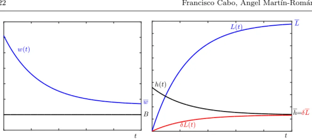
L0 <L¯, employment will increase steadily towards ¯L, as displayed in Figure 4 (right), at the speed|φ|in (24). Correspondingly, as employment grows, the wage determined by the union decays towards a steady-state value greater than the unemployment benefit,B, as shown in Figure 4 (left). Likewise, the firm will hire fewer and fewer employees, while the number of employees who voluntarily quit the firm increases with the level of employment. The reverse holds27 forL0>L¯.
As Figure 4 (right) shows, the two quantities converge, and so employment remains constant at the steady state. An opposite behavior of decreasing em-ployment and increasing wages and recruitment rates would be observed if the
t w(t)
w
B
t h(t)
h=
L(t) L
/L(t)
/L
Fig. 4 Optimal time path for wages (left); hirings and employment (right)
initial level of employment is above the steady state, L0 > L¯. In fact, if L0 is well above ¯L the optimal solution would show an initial period at which the firm fires workers because it needs to reduce employment rapidly. This is followed by a period with positive hiring rates but below the voluntary quit rate (withh(t) converging towardsδL(t) from below).28
The parameters’ values affect the steady-state wages and unemployment rates, as well as the speed of convergence towards the equilibrium, as collected in Table 1. Here we briefly present an example of the effect of the standard symmetric adjustment costs for the firm,c.
Consider the parameters’ values in footnote 26, and assume that the econ-omy is at the steady state, (¯h,w¯) = (.123, .333) with ¯L=.88. At that point, parameterc rises from 0.1 toc0 = 0.15. As a direct effect, the best reaction function for the firm becomes less responsive to wages: ˆh(w,L¯) changes from 3w+ 10(VF)0(.88) to 2w+ 6.66(VF)0(.88). This gives the union an incentive to
raise wages in order to induce more hirings. But this is not the only effect. The marginal valuation of employment rises for the firm and decreases for the union: (VF)
0(.88)−(V
F)
0|
c=c0(.88) =.016, (VU)0(.88)−(VU)0|c=c0(.88) =−.096.
This gives the union the opposite incentive to reduce wages in order to in-duce less hirings. The net effect is a net reduction in wagesw0 =.325< .334, but an increase in hirings, h0 = .183 > .123 and hence ˙L = .051 > 0. The optimal feedback strategies for firm and union (φh(L) = .623−.94L and
φw(L) =.879−.51L) are downward sloping in L. Therefore, as the employ-ment grows, hiring rates and wages decrease towards the new steady state equilibrium (¯h0,w¯0) = (.446, .283) with ¯L=.964. This equilibrium is charac-terized by a lower wage and a higher hiring rate and employment level.
¯
w L¯ |φ|
↑ d ↑ w ↓ L ↓
↑ B ↑ w ↓ L ↔
↑ β ↑ w ↓ L ↑
↑ c ↓ w ↑ L ↓
Table 1 Sensitivity analysis
6 Simultaneous hiring and firing
Up until this point we have assumed that at a given point in time the firm either hires new entrants or fires current workers. In this section we explore the possibility of an equilibrium with some workers being fired and others being recruited at the same time. Such an equilibrium could appear if the benefits associated with the new entrants exceed the adjustment cost linked with the layoff of current employees. To study this possibility, the game between the firm and the union is redefined allowing the firm to determine the number of workers to hire, h+ ≥0, separately from the number of current employees to fire,h− ≥0. The adjustment costs of hiring and firing reflect the same ideas that gave rise to expression (3). The only (but important) difference is that they are defined separately by expressions:29
CF(h
+, w) =c(h+)2
2 −βwh
+, C˜
F(h
−, w) = ˜c(h−)2 2 + ˜βwh
−, c, β,c,˜β >˜ 0.
(25) Parameterβ again represents the relative wage gap, (w(t)−wn(t))/w(t), (as-sumed constant), although it does not necessarily match parameter ˜β, which collects the effect of wages on firing costs. Likewise, c and ˜c can diverge. In order to find a solution in which the firm accepts to pay the cost of firing incumbent workers in exchange for the greater wage savings from the new entrants, we assumeβ >β˜.
Given the adjustment cost functions in (25), the dynamic problem of the firm can be re-written as:
max h+,h−
Z ∞
0
h
Y(L)−wL−CF(h
+, w)−C˜
F(h
−, w)ie−ρtdt, (26)
s.t.:h+≥0, h− ≥0, (27)
s.t.: ˙L=h+−h−−δL, L(0) =L0≥0. (28)
This dynamic problem is subject to algebraic constraints of non-negative con-trol variables in (27), together with the dynamic evolution of the state variable in (28), which now distinguishes between the entrance of new employees and the layoff of current workers.
Following the same reasoning as in Subsection 5.1, the reaction functions of the firm for hiring and firing would be:
ˆ
h+(w, L) = wβ+ (V ±
F )
0(L)
c ,
ˆ
h−(w, L) =−wβ˜+ (V ±
F )
0(L)
˜
c , (29)
withVF±(L) the value function of the firm, conjectured lineal quadratic. Hiring and firing will simultaneously occur if the marginal (positive) value for the firm of reducing employment,−(VF±)0(L), surpasses the marginal firing cost linked with wages, wβ˜. And at the same time, the marginal (negative) value of an additional employee for the firm, (VF±)0(L), does not overcome the profit from the lower wage paid to this new entrant.
Regarding the union, and following the same reasoning that led to the adjustment cost function in (4), now the adjustment cost of hiring and firing is defined by two distinct functions:
CU(h
+) =dh
+(h+−H)
2 ,
˜
CU(h
−) = ˜dh−(h−+ ˜H)
2 ,
˜
d, d >0, (30)
withdandH possibly different from ˜dand ˜H.
The trade union, knowing the firm’s recruitment and layoff policies in (30), solves the dynamic problem:
max w
Z ∞
0
h
wL+ (1−L)B−CU(ˆh
+(w, L))−C˜
U(ˆh
−(w, L))ie−ρtdt, (31)
s.t.: ˙L= ˆh+(w, L)−hˆ−(w, L)−δL, L(0) =L0. (32)
0.69 0.7 0.71 0.72 0.73 0.74 0.75 0.76
t L(t)
0.05 0.0505 0.051 0.0515 0.052 0.0525 0.053
t w(t)
0.28 0.3 0.32 0.34 0.36 0.38 0.4 0.42
t h+(t)
0.07 0.08 0.09 0.1 0.11 0.12 0.13 0.14 0.15 0.16 0.17
t h!(t)
Fig. 5 Time paths with hiring and firing
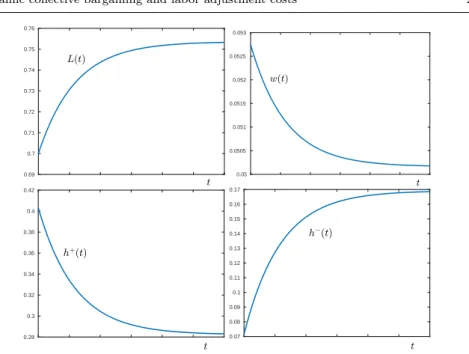
than the influence of wages on firing costs,β >β˜. Thus, the firm has an incen-tive to accelerate the normal turnover implied by those who voluntarily quit in the amounth− >0, in order to increase the number of hired employees h+
above the number of those who voluntarily quit,δL. As Figures 5 show, this is true not only at the steady state, but also along the optimal path. Consider-ing an initially low employment level, the firm hires strongly at the beginnConsider-ing to rise the stock of workers within the firm. Simultaneously, it fires a small number of employees. As the stock of employment approaches its steady-state level, the hiring of new entrants slows down, while the firing of incumbent workers accelerates. At the steady state some workers are fired, ¯h− = 0.12, increasing the amount of workers who can be hired above the amount of those who voluntarily quit, δL¯± = 0.11, to a total hiring rate equal to ¯h+ = 0.23. This example illustrates that hiring and firing can occur simultaneously at the steady state and at any time along the optimal trajectory.
7 Conclusions
Adjustment costs for the firm can be split into the standard symmetric ad-justment costs, plus a wage dependent term. Firing costs are positively affected by the prevailing wage, while hiring actually represents a benefit for the firm under the assumption of wage discrimination to new entrants. Likewise, the union also suffers increasing welfare losses from firings and decreasing welfare gains from hirings.
The baseline scenario considers no adjustment costs for the firm or the union, or equivalently, assumes instantaneous adjustment. Starting from this point, the existence, on the one hand, of adjustment costs for the union would enhance employment while reducing wages if the union strongly welcome new entrants (a marginal rise in hiring above the voluntary quit rate without ad-justment costs increases the union’s welfare). Conversely, if the union very rapidly resents the entrance of new workers, employment would drop while wages rise. On the other hand, the introduction of adjustment costs for the firm could also lead to a reduction in employment, if the benefits from the wage savings associated with the wage gap to new entrants are soft (a marginal rise in hiring above the voluntary quit rate without adjustment costs reduces the firm’s benefits). Conversely, with a strong wage discrimination and a moderate standard part of the hiring costs, employment would conversely augment.
Adding together adjustment costs for the firm and the union allows us to study a richer model. For this game, the sensitivity analysis concludes that employment decreases (and wages augment) with the size of the adjustment costs for the union, and with the unemployment benefits. However, when fo-cusing on the adjustment costs for the firm, a dual conclusion is obtained. A wider wage gap against new entrants reduces employment (and raises wages), while stronger standard symmetric costs increases employment (and reduces wages).
Previous results are obtained considering that the firm either hires or fires workers at a given time. In the final section we allow the firm to take hiring and firing decisions separately. When the benefits for the firm from wage savings are strong with respect to the effect of wages on firing costs, we observe that a solution with simultaneous hiring and firing becomes possible. The firm would agree to pay the firing costs because this would allow an increment in the number of new entrants and, with it, strong gains associated with wage savings.
Appendix
Solutions with adjustment costs only for the firm
– Feedback solution under the assumption w= ¯w, for all t≥0.
Under the assumption ofw= ¯w, and taking into account from (9) that
ˆ
hAF( ¯w, L) = wβ¯ + (V AF F )
0(L)
c ,
the feedback solution to problems (7)-(8) and (10)-(11) is obtained by solving the Hamilton-Jacobi-Bellman equations:
ρVAF
U (L) = ¯wL+ (1−L)B+ (V AF U )
0(L)(ˆhAF( ¯w, L)−δL),
ρVAF
F (L) =aL− L2
2 −wL¯ −c ˆ
h2( ¯w, L) 2 +βw¯
ˆ
h( ¯w, L)
+(VAF F )
0(L)(ˆh( ¯w, L)−δL).
Or equivalently,
ρ(bAF U L+c
AF
U ) = ¯wL+ (1−L)B+b AF U
wβ¯ + (aAF
F L+b AF F )
c −δL
, ρ aAF F L2
2 +b
AF F L+c
AF F
=aL−L 2
2 −wL¯ −
c
2
wβ¯ + (aAF
F L+b AF F ) c
+βw¯wβ¯ + (a
AF F L+b
AF F )
c + (a
AF F L+b
AF F )
¯
wβ+ (aAF F L+b
AF F )
c −δL
.
Identifying quadratic coefficients, linear coefficients and constant terms, in the LHS and the RHS one gets a system of 2+3 algebraic Ricatti equa-tions. The solution to this system of equations is obtained with the help of Mathematica and it is presented in (13) and (14) for the quadratic and the linear coefficients.
– Alternative solutions.
The maximization problem for the union in (10)-(11) with
ˆ
hAF(w, L) = wβ+a AF F L+b
AF F
c ,
is a linear state optimization problem. Therefore, the optimal strategy settled on by the union is assumed constant,w= ¯w for all t≥0. Consequently, for this specific structure of the game, a solution that switches from a to B or vice versa is not feasible.
In Section 4.3 it is proven that the solution ¯w=afor any t≥0 satisfies the necessary conditions for optimality. Conversely, it can be shown that a solution with ¯w=B for anyt≥0 is not optimal. For this solution, expression (14) would implybAF
bywmin =B, unless L(t) remained equal to 0 forever. This solution cannot be optimal because it would imply zero production forever.
A constant wage ¯w∈[B, a] could also appear in a singular path. This type of solution should satisfy:
L(t) =−β
cb AF
U ( ¯w). (33)
From the expressions of aAF F and b
AF
U ( ¯w) in (13) and (14), it immediately
follows that:
bAF U = 2
¯
w−B
ρ+p(ρ+ 2δ)2+ 4/c ≥0 ∀w¯ ∈[B, a].
Thus, from (33), employment should remain constant and either negative or zero along the whole time path, [0,∞). A solution with negative employment is not feasible and a solution with no employment cannot be optimal. Hence, a singular path is not feasible.
Proof of Proposition 1
From (5) and (15) it follows that ¯LAF(ws)< Ls if and only ifβ(a+B)<
δc(a−B), or equivalently, if and only if:
hs≡δLs> βw
s
c .
Moreover, from (15)
( ¯LAF)0(w) =−1−β(ρ+δ)
1 +cδ(ρ+δ) <0.
SincewAF=a > wsthen under condition aboveLs<L¯AF(ws)<L¯AF(a).
Proof of Proposition 2
The expression foraU reads
aU=
−[4c2−dβΦΘ]−√∆
2βΘ ,
withΦ=ρ+ 2δ,Θ= 2(c+d)−dβΦand
∆= [4c2−dβΦΘ]2−4Θ
c2(2c−2d−dβΦ)−2d2β2
.
Under Condition 1,Θ >0, and hence a sufficient condition foraU <0 would
be ∆ > [4c2−dβΦΘ]2, which can be guaranteed under sufficient condition
c≤d.
From the optimal feedback strategies in (21) and (22), one gets
φ1w= c(βaU+c)−dβaF
dβ2 , φ 1 h=
βaU+c dβ .
We have numerically seen that aF >0. Therefore, a necessary condition for φ1
w <0, and a necessary and sufficient condition for φ1h<0, is βaU+c <0.
This expression can be written as
βaU+c=
−4c2+dβΦΘ+ 2cΘ−√∆
2βΘ <0.
Since Θ > 0, a sufficient condition for a negative sign of this expression is −4c2+dβΦΘ+ 2cΘ <0, or equivalently, after some rearrangements
−(dβΦ)2+ 2d(dβΦ) + 4cd <0. (34)
The LHS of this inequality can be interpreted as a second order polyno-mial in dβΦ, with roots: d±√d2+cd. The inequation (34) holds true if
dβΦ < d+√d2+cd. And this condition immediately holds under Condition 1.
Numerical analysis in Section 6
The optimization problem in (26)-(28) is a dynamic problem, subject to the dynamic evolution of the state variable in (28). Furthermore, it is also subject to (algebraic) non-negativity control constraints in (27). To fully characterize the solution one should define a Lagrangian appending the non-negativity constraints to the objective function with their corresponding multipliers, and then derive the necessary conditions including Kuhn-Tucker conditions. Our approach has been to solve the problem (with the help of Mathematica) for the parameters’ values specified, ignoring the non-negativity constraints, and once the solution is found check whether these conditions are indeed satisfied. The Hamilton-Jacobi-Bellman equation associated with problem (26)-(28) is:
ρVF±(L) = max h+,h−
aL−L 2
2 −wL−c (h+)2
2 +βwh
+−c˜(h−)2 2 + ˜βwh
−+
(VF±)0(L)(h+−h−−δL) .
From this equation, the reaction functions in (29) immediately follow. Plugging these policies into the union’s maximization problem, the dynamic problem (31)-(32) is obtained. The Hamilton-Jacobi-Bellman equation for this problem is:
ρVU±(L) = max w
(
wL+ (1−L)B−d
ˆ
h+(w, L)(ˆh+(w, L)−H)
2 −
˜
d
ˆ
h−(w, L)(ˆh−(w, L) + ˜H)
2 + (V
±
U )
0(L)(ˆh+(w, L)−hˆ−(w, L)−δL)
)