Degeneracy in carbon nanotubes
under transverse magnetic
δ
-fields
S¸. Kuru∗1
, J. Negro †2
, and S. Tristao‡2 1
Department of Physics, Faculty of Science, Ankara University. 06100 Ankara, Turkey
2
Departamento de F´ısica Te´orica, At´omica y ´Optica, and IMUVA (Instituto de Matem´aticas), Universidad de Valladolid. E-47011 Valladolid, Spain
Abstract
The aim of this paper is to study the degeneracy of the energy spectrum in a nanotube under a transverse magnetic field. The massless Dirac-Weyl equation has been used to describe the low energy states of this system. The particular case of a singular magnetic field approximated by Dirac delta distributions is considered. It is shown that, under general symmetry conditions, there is a degeneracy corresponding to periodic solutions with a null axial momentumkz= 0. Besides, there may be present
a kind of sporadic degeneracy for non-vanishing values of kz, which are explicitly
computed in the present example. The proof of these properties is obtained by means of the supersymmetric structure of the Dirac-Weyl Hamiltonian.
Keywords: Massless Dirac-Weyl equation, nanotube, spectrum degeneracy, super-symmetry.
1
Introduction
Single walled carbon nanotubes (CN) can be considered as a sheet of graphene rolled up to form a cylinder. Depending on the angle of the graphene lattice and the cylinder axis, the nanotube will inherit a metallic or semiconducting character [1–4].
The application of magnetic fields to a nanotube can have two kinds of effects. If the field is longitudinal (in the direction of the nanotube axis) it may interchange metallic and semiconducting behaviors by opening (or reducing) a gap in the band center. On the other
∗email:
†email:
hand, transverse magnetic fields in general will increase the metallic character by reducing the initial gap [4–9].
The description of the low energy states of nanotubes, near each of the two Fermi points, can be done in the continuous limit of a tight binding model by means of the massless Dirac-Weyl equation, provided the circumference length L= 2πρ0 is much larger than the C-C
distance a [4]. In the presence of a magnetic field of intensity B, the interaction can be described by the minimal coupling rule in the Dirac equation if qB~c is much larger than
aρ0, in order to avoid lattice effects [7]. The different types of nanotubes can be taken into
account in the continuum limit by means of certain quasi-periodic conditions [4].
In this paper we will make use of this picture of low energy states to study the interaction of a nanotube with a singular transverse magnetic field that can be approximated by a Dirac delta. We want to address the question of the degeneracy of the energy spectrum. There are many references dealing with the electronic properties of nanotubes in transverse magnetic fields, but in general the problem of degeneracy has not been fully explained. For instance, in [7] it is given a discussion on this point in order to show a quantum Hall effect in nanotubes, but this is done on a rather qualitative ground. We want to deduce the degeneracy properties just from the symmetries of the periodic Dirac-Weyl equation. The natural way to get a satisfactory answer to this problem is by making use of supersymmetry arguments. Each component of the Dirac spinor satisfies an effective Schr¨odinger equation of a supersymmetric couple [10]. The connection of the symmetry properties of these two effective equations will lead us to a global symmetry explaining the degeneracy.
2
Nanotube in external magnetic fields
We will start with the general formalism to describe the quasi-particles of a nanotube in a magnetic field at low energies. In principle, the magnetic field at each point of the nanotube surface can be decomposed into transverse B⊥ (perpendicular to the surface)
and parallel Bk (tangent to the surface) components. As the Lorentz force produced
by the magnetic field is perpendicular to the motion of the charged particles, only the perpendicular component is effective in this situation. The other components, specially the longitudinal component along the nanotube axis, may have another kind of influence that will not be considered here [5, 6, 9, 11].
Let us take cylindrical coordinates (ρ, φ, z), where thez-axis is along the nanotube axis. Since the magnetic fieldB produced by the vector potentialA=Aρnρ+Aφnφ+Aznz is
B=∇ ×A=
1
ρ∂φAz−∂zAφ
nρ+ (∂zAρ−∂ρAz)nφ+
∂ρAφ−∂φAρ+
Aφ
ρ
nz (1)
then, the effective magnetic field perpendicular to the nanotube surface at ρ=ρ0 will be
given by
B⊥=
1
ρ0
∂φAz−∂zAφ
nρ. (2)
This effective field can be described by a vector potential tangent to the surface of the nanotube,
A=Aφ(φ, z)nφ+Az(φ, z)nz. (3)
In the low energy limit, a quasi-particle interacting with the effective magnetic fieldB⊥ is
described by the massless Dirac-Weyl equation [4, 11] via the minimal coupling with the vector potential (3),
−σ2
i∂z+
q c~Az
+σ1
i ρ0
∂φ+
q c~Aφ
ˆ
Ψ(z, φ) =ǫΨ(ˆ z, φ), (4)
whereǫ= E
vF~. Now, the wave functions ˆΨ(z, φ) that we are looking for are subject to the
boundary condition
ˆ
Ψ(z,2π) =ei2πδΨ(ˆ z,0), (5) where−1/2 < δ≤1/2 is the phase shift after a period of the angular variable. Since the values δ and −δ are related by a complex conjugation in (5), hereafter we will restrict to positive values 0≤δ ≤1/2. The concrete value of δ to be considered will depend on the properties of the nanotube: it is related to the particular way a piece of planar graphene is rolled in order to construct the nanotube or to other longitudinal magnetic fields [4].
Here, we will deal with the case whereB⊥ does not depend on zbut it is a function of
φ. This situation can be described by the potential
(Aφ= 0, Az =Az(φ)) =⇒ B⊥(φ) =
1
ρ0
Due to the symmetry under translation in thez-direction, the stationary equation (4) can be separated by taking the wave function in the form
ˆ
Ψ(z, φ) =eikzzΨ(φ), Ψ(φ) =
ψ1 (φ) ψ2 (φ) . (7)
Thus, we get a one dimensional stationary equation depending on the constant momentum
pz =~kz of the particle in thez-direction,
h
iσ1∂φ+
ρ0kz−
ρ0q
c~ Az(φ)
σ2
i
Ψ(φ) =ρ0ǫΨ(φ), (8)
together with the boundary condition
Ψ(φ+ 2π) =ei2πδΨ(φ), 0≤δ≤1/2. (9)
Equation (8) represents two coupled, first-order differential equations for the spin-up and down componentsψ1
(φ) and ψ2
(φ), respectively. Let us introduce the operators
A† = ∂φ+W(φ), A=−∂φ+W(φ), (10)
where
W(φ) =−ρ0kz+
ρ0q
c~Az(φ). (11)
In terms of these operators, equation (8) can be cast in a more appealing form:
HΨ(φ) =
0 iA†
−iA 0
Ψ(φ) = ˜ǫΨ(φ), ˜ǫ=ρ0ǫ . (12)
This equation can be decoupled by applying H to the left, so that we obtain a diagonal second order HamiltonianH2,
H2Ψ(φ)≡
H1 0
0 H2
Ψ(φ) =
A†A 0
0 AA†
Ψ(φ) = ˜ǫ2Ψ(φ) (13)
where
H1≡A†A=−∂φ2+W2(φ) +
dW(φ)
dφ , H2≡AA
†=−∂2
φ+W
2
(φ)−dW(φ)
dφ . (14)
Therefore, the upper (ψ1
) and lower (ψ2
) components of Ψ(φ) must be eigenfunctions of the effective Schr¨odinger Hamiltonians H1 and H2, respectively, with the same effective
energy ˜ǫ = ρ2 0ǫ
2
. If the eigenvalue is nonzero, according to (12) these components are related by means of the operators (10),
ψ1 = i ˜
ǫA †ψ2
, ψ2=−i
˜
ǫAψ
1
The zero modes Ψ0 = (ψ01, ψ 2
0)T of the HamiltonianHcan be found by solving the following
equations
A†ψ02 = 0, Aψ01= 0. (16)
Only when the solutions to these 1st order equations satisfy the boundary conditions, they give rise, respectively, to the zero energy solutions
Ψ↑0 =
ψ1 0
0
, Ψ↓0 =
0
ψ2 0
. (17)
In the frame of supersymmetric quantum mechanics, we say that the Hamiltonians H1
and H2 are supersymmetric partners, the operators A,A† are intertwining operators and
the functionW(φ) is the superpotential. The spectral problem for the matrix Hamiltonian (12) is equivalent to that of the common spectrum of the scalar HamiltoniansH1 and H2
given in (14). The effective potentials of these scalar Hamiltonians are given, according to (14), by
V1(φ) =W2(φ) +
dW(φ)
dφ , V2(φ) =W
2
(φ)−dW(φ)
dφ . (18)
These scalar potentials will help us to interpret the behavior of the componentsψ1
(φ) and
ψ2
(φ) in the original matrix equation (12). The boundary conditions on the eigenfunctions
ψ1,2(φ) of the scalar Hamiltonians are the same as in (9),
ψ1,2
(φ+ 2π) =ei2πδψ1,2
(φ), 0≤δ≤1/2. (19)
3
Transverse magnetic
δ
-fields
We will consider a magnetic field that enters in the nanotube near the pointφ=π/2 with a singular intensity given in terms of the Dirac delta distribution, and leaves the nanotube at the opposite point φ = −π/2 with the same intensity. This field is described by the magnetic potential
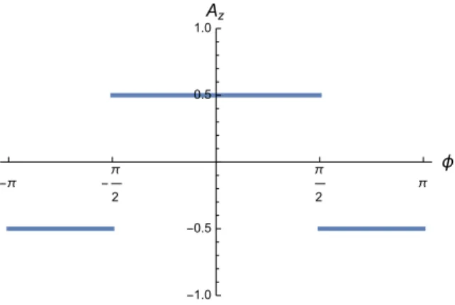
Az(φ) =A0 [H(φ+π/2) +H(−φ+π/2)−3/2], −π≤φ≤π , (20)
where H(φ) is the Heaviside function (see Fig. 1). Then, according to (6), the magnetic field has the expression
B⊥= A0
ρ0
δ(φ+π/2)−δ(φ−π/2)
nρ≡B(φ)nρ. (21)
There are two important aspects of the potential function to be remarked.
(i) Asφis an angular variable, the potentialAz(φ) in (20) can be extended to a periodic
Figure 1: The potentialAz(φ) given in (20) forA0= 1.
(ii) The integral of Az(φ) along a period vanishes:
R2π
0 Az(φ)dφ= 0 .
The next step is replacing this magnetic potential in the eigenvalue equation (26) for the effective Hamiltonians H1 and H2 with effective potentials (18). It will be useful to
introduce the following constants
α=ρ0kz, β =
ρ0q
c~ (22)
so that
W(φ) =−α+β Az(φ). (23)
Notice that, once fixed the radius of the nanotube, the parameter αis proportional to the momentumkz in thez–direction. Then, the explicit form of the effective potentials is (see
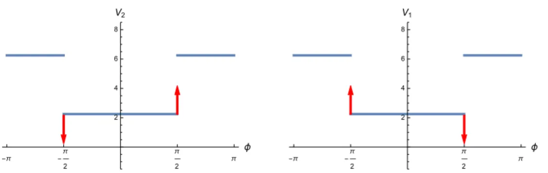
Fig. 2)
V1(φ) =α2+
β2
A2 0
4 −2βαAz(φ) +βρ0B(φ) =V0(φ) +βρ0B(φ), (24)
V2(φ) =α2+
β2
A2 0
4 −2βαAz(φ)−βρ0B(φ) =V0(φ)−βρ0B(φ). (25) Thus, the effective potentials include two terms:
(i) A common term,V0(φ), with a part proportional to the magnetic potential,−2βαAz(φ),
plus a constantM ≡α2
+β
2
A2 0
4 (depending onkz andρ0).
(ii) A second term proportional to the magnetic field intensity: ±βρ0B(φ) (with plus
sign forV1 and minus sign forV2). This term contains the Dirac delta singularities.
In order to solve the spectral problem, we can choose just one of the Hamiltonians H1
Figure 2: Effective potentials V2(φ) (left) and V1(φ) (right) for α = 2, β = 1, A0 = 1. The δ singularities are represented by arrows at the discontinuity points.
Henceforth, we will takeH2 and write down its eigenvalue equation:
H2ψ(φ) = ˜ǫ2ψ(φ), ψ(φ)≡ψ2(φ). (26)
This equation can be divided in the three regions of the interval [−π, π] where the finite potential V0 takes constant values (see Fig. 2):
V0(φ) =
M+N, −π < φ <−π/2 (I)
M−N, −π/2< φ < π/2 (II)
M+N, π/2< φ < π (III)
M =α2+β
2A2 0
4 , N =βαA0.
(27) If α → 0, then N → 0, so that in this case V0(φ) will remain constant and the only
significant contribution to the effective potential will come from the singular magnetic field.
The solutions corresponding to a fixed effective energy ˜ǫ2consist of the free Schr¨odinger
solutions in the three regions subject to appropriate matching and periodic conditions,
h
d2
dφ2 −κ1
2i
ψI(φ) = 0, −π < φ <−π/2, κ12 = (M +N)−˜ǫ2
h
d2
dφ2 −κ22
i
ψII(φ) = 0, −π/2< φ < π/2, κ22 = (M −N)−˜ǫ2
h
d2
dφ2 −κ12
i
ψIII(φ) = 0, π/2< φ < π, κ12 = (M+N)−˜ǫ2.
(28)
The matching conditions at φ=±π/2 are determined by the Dirac delta singularities of the magnetic term of the potential at these points:
ψI(−π/2) =ψII(−π/2), ψII(π/2) =ψIII(π/2),
ψ′I(−π/2) =ψII′ (−π/2) +βA0ψI(−π/2), ψ′II(π/2) =ψIII′ (π/2)−βA0ψI(π/2).
Besides, there must be added the periodicity conditions at φ=±π:
ψIII(π) =ei2πδψI(−π), ψIII′ (π) =ei
2πδψ′
I(−π). (30)
When solving this problem, one must have in mind that there are three types of values the effective energy ˜ǫ2
can take (here we are assumingα >0):
(i) ǫ˜2
> M+N, (ii) M+N >˜ǫ2
> M−N, (iii) M−N >˜ǫ2
. (31)
3.1 Periodic solutions
If we choose δ = 0, we get the periodic solutions. This situation corresponds to the case where the lattice consists in hexagons matching well around the nanotube [4]. In this case, the longitudinal field is also vanishing. We have to solve the spectrum in the three different ranges of the effective energy mentioned above. This is given by the following simple formulas:
˜
ǫ2 > M +N, κ
j =ikj, j= 1,2
k1(2k1k2(−1 + cos(k1π) cos(k2π)) + (A20β 2+k2
1 +k 2
2) sin(k1π) sin(k2π)) = 0,
M+N >˜ǫ2
> M −N, κ1 =k1, κ2 =i k2
k1(2k1k2(−1 + cosh(k1π) cos(k2π))−(A20β 2
−k2 1 +k
2
2) sinh(k1π) sin(k2π)) = 0,
M−N >˜ǫ2
, κj =kj, j= 1,2
k1(2k1k2(−1+ cosh(k1π) cosh(k2π)) + (−A20β 2
+k2 1+k
2
2) sinh(k1π) sinh(k2π)) = 0.
(32)
The plot of the resulting spectrum as a function of the ‘momentum’ α is displayed in Fig. 3 for three values of the field intensity,A0 = 1,5,10. This is similar to Fig. 2 of Ref. [7]
for constant magnetic fields. The most important feature, regarding the degeneracy, is that all the energy levels, for any magnetic field intensity, are degenerate at kz = 0 (α = 0).
Notice that forkz = 0 the two effective potentials (24) and (25) are simpler:
V1(φ) =
β2
A2 0
4 +βρ0B(φ), V2(φ) =
β2
A2 0
4 −βρ0B(φ). (33) This means that both,V1(φ) andV2(φ), are symmetric with respect to the reflection around
the singular pointsφn =−π2 +n π. We will show in the next section that, indeed in this
situation the energy levels of the periodic solutions must be degenerate.
When |kz| > 0 this symmetry is broken, the degeneration is lifted and all the levels
become non-degenerated. However, for greater values of |kz| there can appear ‘sporadic’
degeneracies at certain values of |kz| as can be appreciated in Fig. 3. The reason is that
Figure 3: Spectrum of the energies ˜ǫ = ρ0
vF~E of periodic solutions as functions ofα= ρ0kz for
different intensities of the magnetic field (21): A0 = 1 (left), A0 = 5 (center), A0 = 10 (right) in units of ρ0q
c~ (this is equivalent to set β = 1 in (27)). The dotted lines in black correspond to the
valuesM +N,M −N of the finite part (27) of the effective potentials V1, V2.
potentialsV1 and V2 are related by means of a reflection, V1(φ) =V2(−φ). As we will see
later, this property will be the origin of sporadic degeneracies in this case.
In Fig. 3 it is also shown the effect of increasing the intensity of the magnetic field on the spectrum. The gap of the central energy levels is reduced even for larger values of kz
as the magnetic field is bigger. Thus, the metallic behavior is strengthened by the intense magnetic fields [4, 7].
Of course, we should also mention the trivial symmetry of the spectrum with respect to the sign ofkz.
Once we know the spectrum and solutions for periodic functions, we can compute the density current jz in the direction of the nanotube axis. According to the notation of (7)
this is given by
jz = ˆΨ(z, φ)†σ2Ψ(ˆ z, φ) = Ψ(φ)†σ2Ψ(φ). (34)
The componentsψ1
and ψ2
of Ψ are related by (15),ψ1
= ˜ǫiA+ψ2, as far as ˜ǫ6= 0 (in case
˜
ǫ= 0 the density current will vanish). The componentψ2
will be a solution of the effective Hamiltonian H2 as written in (26) and in the periodic case it can always be chosen real.
Replacing these components in (34) we have
jz(φ) =−
2 ˜
ǫψ
2A+
ψ2
. (35)
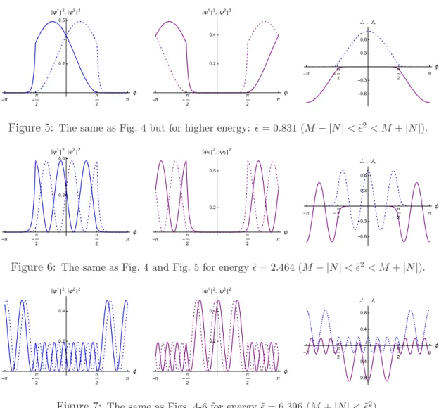
Now, we are in conditions to compute the density current for any periodic solution of the above spectrum. In Figs. 4–7 it is shown the wavefunctions and their corresponding currents of periodic solutions forα=±3,A0 = 5 at four different energies.
Due to the relation of the total current with the dispersion relation [7], when kz = 0
we will have
Z 2π
0
Figure 4: Squared wave-functions corresponding to positiveαat the left in blue, and to negativeα at the center in purple. The corresponding current densities are shown at the right (for positiveα in dashing blue, forαnegative in continuous purple line). Values: α=±3, β= 1, A0= 5,˜ǫ= 0.018 (˜ǫ2
< M − |N|).
Figure 5: The same as Fig. 4 but for higher energy: ˜ǫ= 0.831 (M− |N|<˜ǫ2
< M+|N|).
Figure 6: The same as Fig. 4 and Fig. 5 for energy ˜ǫ= 2.464 (M − |N|<˜ǫ2
< M+|N|).
Figure 8: Spectrum of the energies ˜ǫof anti-periodic solutions as functions ofα=ρ0kzfor different
values of the magnetic field: A0= 1 (left),A0= 5 (center),A0= 10 (right) andβ = 1. The dotted curves in black correspond to the valuesM+N andM−N of the finite part (27) of the effective potentialsV1, V2.
However, for kz > 0 (kz < 0) the net current is positive (negative), and it becomes
larger as we increase kz. This phenomenon describes a non null flux of charged particles
corresponding to axial linear momentumkz. It should be remarked that while the positive
current for positive values kz > 0 is restricted to one of the subintervals |φ| < π/2 or
π > |φ| > π/2, the current for negative values kz < 0 will be present just in the other
subinterval. Thus, it is like having a highway with two separate lanes, each one for a different sign of kz carrier.
3.2 Anti-periodic solutions
The anti-periodic solutions are obtained for the value δ = 1/2. The equations for the matching and anti-periodic conditions are similar to the previous case (32). A plot of the resulting spectrum is given in Fig. 8 for three different values of the magnetic field. It is shown that, for low field intensities (A0 ≈ 1), at kz = 0 the spectrum is not degenerated
(contrary to the periodic case). An example of anti-periodic solution atα= 0 is represented in Fig. 9. As the field intensity becomes higher the lowest energy level becomes degenerated, thus enhancing the metallic character (see in Fig. 8 the plots in the center and to the right). We can also observe that when|kz|is increasing some ‘sporadic’ degeneration can appear
Figure 9: Components of the anti-periodic eigenfunction Ψ = (i ψ1 , ψ2
)T (left) atα= 0, for an
effective energy ˜ǫ = √2.18 with β = 1, A0 = 1 (left). The (real part of) first component ψ1 is represented by a dashing line while the second oneψ2
is in continuous curve, the density current j(φ) is on the right.
4
Degeneracy of the spectrum
4.1 Degeneracy of the spectrum of periodic solutions at kz = 0
As remarked above, whenkz = 0 the spectrum of periodic solutions is degenerated. In this
section we will explain the reason for the degeneracy as well as why this degeneracy does not affect to other solutions (for instance, to anti-periodic solutions). The proof of this property lies in the supersymmetric character of the effective Hamiltonians given by (14) in terms ofW(φ). According to (11) ifkz = 0 the superpotentialW(φ) coincides, up to a
multiplicative constant, just with the magnetic potentialAz (20),
W(φ) =β Az(φ). (37)
In this situation, let us enumerate the symmetry properties ofW(φ) which are immediate from Fig. 1 (the angular variable φis assumed to range overR):
(i) Periodicity with period T = 2π:
W(φ) =W(φ+ 2π). (38)
(ii) Anti-symmetry with respect to reflections around the pointsφn= π2 +n π,n∈Z:
W(φ+φn) =−W(−φ+φn). (39)
(iii) Anti-periodicity with anti-periodA=π:
W(φ) =−W(φ+π). (40)
Figure 10: Components of two independent periodic eigenfunctions Ψ = (i ψ1 , ψ2
)T (left) and
˜
Ψ = (iψ˜1 ,ψ˜2
)T (center) for a degenerated effective energy ˜ǫ=√4.25 at α= 0 with β= 1, A 0= 1. The (real part of) the first componentsψ1
and ˜ψ1
are represented by dashing lines while the second onesψ2
and ˜ψ2
are in continuous lines. Density currentsj(φ),˜j(φ) for the solutions Ψ (continuous) and ˜Ψ (dashing) are represented to the right.
(i′) Both potentials V
1, V2 are periodic with periodT = 2π:
Vi(φ) =Vi(φ+ 2π), i= 1,2. (41)
(ii′) Both potentials V1, V2 are symmetric with respect to reflections around the points
φn= π2 +n π,n∈Z:
Vi(φ+φn) =Vi(−φ+φn), i= 1,2. (42)
(iii′) The partner potentials V1, V2 areπ-displaced from each other:
V1(φ) =V2(φ+π). (43)
To prove the properties (i′)-(iii′) from (i)-(iii) it is enough to make use of the defining formulas (18) ofV1, V2 in terms of W(φ).
Now, let us concentrate in the periodic solutions of Hamiltonian H2 with potential V2
characterized by the above properties. SinceV2 isφn–symmetric, which is compatible with
the 2π–periodicity, this implies that we can classify each periodic solution inφn–symmetric
or φn–anti-symmetric. This means, for example, that if ψ is both 2π-periodic and φ0
-symmetric, then necessarily it should also beφn–symmetric for alln∈Z. Or if ψis both
2π–periodic andφ0–anti-symmetric, then necessarily it should also be φn–anti-symmetric ∀n∈Z. As an example, the periodic solutionψ
2
shown in Fig. 10 (left, continuous curve) isφn–symmetric while ˜ψ2 isφn–antisymmetric (center, continuous curve).
Let ψ2
be a 2π-periodic eigenfunction of H2, such that for example, it is also φn
-symmetric. Then, according to (15), the function ψ1
= i˜ǫA†ψ
2
will be a solution of H1.
Since A†(φ) is a φn–anti-symmetric operator, the resulting function ψ1 will be φn
–anti-symmetric. Therefore, the symmetric/antisymmetric character of ψ1
is opposite to that of ψ2
. For example, in Fig. 10 (left) it is seen that the periodic solution ψ1
(dashing) is
On the other hand, from property (iii′) (43), as H1(φ+π) = H2(φ), we have that
˜
ψ2
(φ) =ψ1
(φ+π) is an eigenfunction ofH2(φ). Therefore, we have the initial eigenfunction
ψ2(φ) and the new eigenfunction ˜ψ2(φ) ofH
2. As each of these eigenfunctions has different
character to the other (one is φn-symmetric while the other is φn–anti-symmetric), they
must be independent, and therefore the eigenvalue is degenerate. As an illustration, the eigenfunctions ψ2 and ˜ψ2, shown in Fig. 10, correspond to the same eigenvalue and they
have differentφn–symmetric/anti-symmetric character.
Now, let us consider briefly the case of anti-periodic eigenfunctions of H2. In this
case the functionψ2 satisfies ψ(φ+ 2π) =
−ψ(φ). If ψ2 is φ
0-symmetric, due to the
anti-periodicity it will be anti-symmetric with respect toφ1 =φ0+π. Then, it is easily seen that
ψ2
will be [φ0+ 2nπ]–symmetric and [φ0+ (2n+ 1)π]–anti-symmetric. When we compute
the eigenfunction ψ1
of H1 by ψ1 = i˜ǫA†ψ2, this eigenfunction will change the character
in φ0 so that it will be [φ0 + 2nπ]–anti-symmetric and [φ0+ (2n+ 1)π]–anti-symmetric.
From ψ1
we can get an eigenfunction of H2 by translation: ˜ψ2(φ) = ψ1(φ+π). In this
way we get a new eigenfunction ˜ψ2 that has the same symmetric character as the initial
ψ2
. Therefore, as they could be proportional we can not say whether they are linearly dependent or independent. In other words, the symmetry does not tell us anything about the degeneracy of the spectrum of anti-periodic eigenfunctions. An example of anti-periodic eigenfunction for α = 0 is given in Fig. 9, where it is shown the mixed symmetric/anti-symmetric character of the componentsψ1
(φ), ψ2
(φ) around the points φn=±π/2.
4.2 Sporadic degeneracy for kz 6= 0
Besides the degeneracy for periodic solutions that applies to the case α = 0, there is another type of degeneracy for both periodic and anti-periodic solutions, which depends on the values of the parameters α 6= 0 and ˜ǫ. For instance, one can appreciate in Fig. 3 (left) that for the value (α= 4,ǫ˜= 4.61) there must be a degeneracy of periodic solutions, while in Fig. 8 (left), the values (α= 1.5,˜ǫ= 2.23), (α= 2.5,ǫ˜= 3.6), (α= 3.5,ǫ˜= 5) will correspond to degenerate anti-periodic solutions. As this new type of degeneracy will be present only for some specific pair of values of (α,ǫ˜), it will be called ‘sporadic’.
The origin of the sporadic degeneracy relies in the symmetry relation V1(−φ) =V2(φ),
as can be seen in Fig. 2. The procedure to characterize the sporadic degeneracy values (α,˜ǫ) consists in the following steps.
a) Find a symmetric or anti-symmetric solution ψ2
of H2 for an specific pair of values
(α,ǫ˜) (if it does exist!).
b) By means of the operator A+, following the relation (15), construct the associate
solution ψ1
of H1. Since W(φ), given in (23), has no symmetry for α 6= 0, the
solutionψ1
will not be symmetric nor anti-symmetric.
c) As H1(−φ) =H2(φ), a second solution ˜ψ2 of H2 will be given by ˜ψ2(φ) =ψ1(−φ).
Then, ˜ψ2
and ψ2
must be linearly independent since the initial function ψ2
sym-metric or anti-symsym-metric while ˜ψ2
is not. In conclusion, for such values (α,˜ǫ) there will be a degeneracy given byψ2
and ˜ψ2
.
Therefore, according to the above procedure, in order to obtain an sporadic degeneracy, it is enough to compute particular solutions with an even/odd symmetry. Such a type of solutions can be found in a simple way for our particular magnetic field.
Consider for instance the case of anti-periodic solutions. An even anti-periodic solution is given, for example, by (we hare restricting to the case ˜ǫ2
> M +N,α >0)
ψ2(φ) =
(−1)n k2
k1 sin(k1(φ+π/2)), −π < φ <−π/2, k1= 2n
cos(k2φ), −π/2< φ < π/2, k2= 2n+ 1
−(−1)n k2
k1 sin(k1(φ−π/2)), π/2< φ < π, k1= 2n
n∈N.
(44) This type of functions satisfy the matching conditions (29). According to the values of k1
and k2 for the solutions given in (28), they are determined by the equations
(
k2 1 = ˜ǫ
2
−(M+N) = (2n)2
k2 2 = ˜ǫ
2
−(M−N) = (2n+ 1)2
. (45)
Once fixed the integer value nand, for example, the parameters β = 1, A0 = 1, then the
two equations (45) will give us the values (˜ǫ, α) of the corresponding sporadic degeneracy:
Degenerate even solutions : (α= 2n+1 2, ˜ǫ
2
= 8n2+ 4n+ 1), n∈N. (46)
Odd anti-periodic solutions are given, for instance, by (also in the case ˜ǫ2
> M+N,α >0)
ψ2 (φ) =
(−1)n k2
k1sin(k1(φ+π/2)), −π < φ <−π/2, k1= 2n−1
sin(k2φ), −π/2< φ < π/2, k2= 2n
(−1)n k2
k1sin(k1(φ−π/2)), π/2< φ < π, k1= 2n−1
n∈N.
(47) This time, once fixedn, β, A0, the degeneracy values ofα,˜ǫare given by
(
k2 1 = ˜ǫ
2
−(M +N) = (2n−1)2
k2 2 = ˜ǫ
2
−(M −N) = (2n)2
. (48)
Hence, in this example, for β= 1, A0 = 1, the degeneracy values are
Degenerate odd solutions : (α= 2n− 1
2, ˜ǫ
2
Figure 11: Anti-periodic functions of a ‘sporadic’ degenerate energy ˜ǫ=√5,α= 1.5, β= 1, A0= 1. The first anti-periodic eigenfunction Ψ = (ψ1
, ψ2
)T is plotted to the left and the second ˜Ψ =
( ˜ψ1 ,ψ˜2
)T to the right. The first components ψ1 ,ψ˜1
are represented by dashing curves while the second ones ψ2
,ψ˜2
are in continuous curves. Remark that ψ2
is an odd anti-periodic function as mentioned in (50).
According to (46) and (49), the first values of sporadic degeneracy of anti-periodic solutions are therefore:
(α= 1.5, ˜ǫ2
= 5), odd (α= 2.5, ˜ǫ2
= 13), even (α= 3.5, ˜ǫ2
= 25), odd.
(50)
Such values can be observed in Fig. 8 (left). The independent solutions for the first case (α= 1.5,ǫ˜2
= 5) are shown in Fig. 11.
The case of sporadic degeneracy for the periodic solutions can be studied in a similar way. Just for completeness we will supply the first sporadic periodic values forβ = 1, A0 =
1,
Even solutions : (α= 4n, ˜ǫ2
= 20n2
+54), n= 1,2, . . .
Odd solutions : (α= 4n−2, ˜ǫ2
= 20n2
−20n+ 6 +14), n= 2,3, . . .
(51)
The first value of degeneracy is the even solution (α = 4,ǫ˜2 = 21.25), which can be
appreciated in Fig. 12 (left). Following this procedure in a straightforward way, a complete list of all the sporadic degeneracies can be given for this magnetic field.
5
Conclusions
Figure 12: Periodic functions of a ‘sporadic’ degenerate energy ˜ǫ=√21.25,α= 4, β = 1, A0= 1. The first anti-periodic eigenfunction Ψ = (ψ1
, ψ2
)T is plotted to the left and the second ˜Ψ =
( ˜ψ1 ,ψ˜2
)T to the right. The first components ψ1 ,ψ˜1
are represented by dashing curves while the second ones ψ2
,ψ˜2
are in continuous curves. Remark that ψ2
is an even periodic function as mentioned in (51).
in different configurations related to graphene [12, 13], where our considerations can be extended for the periodic cases.
The main conclusion is that there exists degeneracy for the periodic solutions corre-sponding to null axial momentumkz = 0. This type of degeneracy is present under quite
general symmetry conditions, so that it is also found, for example, in the case of a constant background magnetic field as given in [4, 7] or in elliptic potentials [11]. There can be another type of more restricted degeneracy that we call ‘sporadic’. This new degeneracy is present in our example for some periodic and anti-periodic solutions, but it depends on very special conditions of the magnetic field.
The degeneracy of energy levels has important effects on the electronic properties of the nanotube. In the case of the degeneracy forkz = 0 and high field intensities, it persists for
the ground level even when|kz|>0 (see Fig. 3), which gives rise to an special quantum Hall
effect for thick nanotubes [7]. The sporadic degeneracy is only present in higher levels, so its consequences are not so evident. However, the sporadic degeneracy leads to an increase of the density of states and it will also drastically affect to the current properties for the corresponding specific values of (E, kz). In the case of periodic magnetic fields in graphene,
where our considerations still apply, the sporadic degeneracy will suppress a forbidden band at the degenerating values of (E, kz) giving rise to a wider allowed band.
Acknowledgments
We acknowledge financial support from Spanish MINECO, project MTM2014-57129. S¸. Kuru acknowledges the warm hospitality at Department of Theoretical Physics, University of Valladolid, Spain.
References
[1] R. Saito, G. Dresselhaus and M. S. Dresselhaus, Physical properties of carbon
nan-otubes (Imperial College Press, London, 1998).
[2] J. -C. Charlier, X. Blase and S. Roche, Rev. Mod. Phys.79, 677 (2007) and references
therein.
[3] C.L. Kane and E.J. Mele, Phys. Rev. Lett. 78, 1932 (1997).
[4] H.-W. Lee, Dmitry S. Novikov, Phys. Rev. B 68, 155402 (2003).
[5] H. Ajiki and T. Ando, J. Phys. Soc. Jpn.62, 1255 (1993).
[6] J. P. Lu, Phys. Rev. B 74, 1123 (1995).
[7] E. Perfetto, J. Gonz´alez, F. Guinea, S. Bellucci and P. Onorato, Phys. Rev. B 76,
125430 (2007).
[8] S. Bellucci, J. Gonz´alez, F. Guinea, P. Onorato and E. Perfetto J. Phys.: Condens. Matter 19, 395017 (2007).
[9] N. Nemec and G. Cuniberti, Phys. Rev. B74, 165411 (2006).
[10] S¸. Kuru, J. Negro and L.M. Nieto, J. Phys.: Condens. Matter 21, 455305 (2009).
[11] V. Jakubsky, S¸. Kuru and J. Negro, J. Phys. A: Math. Theor. 47, 115307 (2014).
[12] M. Ramezani Masir, P. Vasilopoulos and F.M. Peeters, New J. Phys. 11, 095009
(2009).
[13] S. Ghosh and M. Sharma, J. Phys.: Condens. Matter 21, 292204 (2009).
[14] V. Jakubsky, S¸. Kuru, J. Negro and S. Tristao, J. Phys.: Condens. Matter 25, 165301
(2013).