Design and application of measuring techniques for the validation of models for high pressure induced solid liquid transition

UNIVERSIDAD DE VALLADOLID

ESCUELA DE INGENIERIAS INDUSTRIALES

Grado en Ingeniería Química

Design and application of measuring

techniques for the validation of models for

high-pressure induced solid-liquid transition

Autor:

Cuadrado Llorente, Marta

Gloria Esther Alonso Sánchez

Friedrich

_-

Alexander

_{-Universität Erlangen-Nürnberg}

TFG REALIZADO EN PROGRAMA DE INTERCAMBIO

TÍTULO: Design and application of measuring techniques for the validation of models for high-pressure induced solid-liquid transition

ALUMNO: Marta Cuadrado Llorente

FECHA: 08/08/2017

RESUMEN Y PALABRAS CLAVES

Gas hydrates, viscosidad, densidad, industria alimentaria, zumos.

Los gases hidratados son unos compuestos, en lo que la molécula de agua, es el hogar de una molécula de gas.

Desde el punto de vista de la industria alimentaria, estos gases hidratados están siendo estudiados para los procesos de concentración de zumos, añadiendo dióxido de carbono como molécula gas, alcanzando un 99% de concentración del zumo y preservando la naturaleza de nuestro producto sin dañar las vitaminas existentes.

Para saber como los gases hidratados se van a comportar en su formación, ya que van a pasar por diferentes estados de presión y temperatura, hay que realizar un estudio de sus propiedades más significativas, la densidad y la viscosidad. Esos experimentos se realizaran con disoluciones de agua más azúcar, a diferentes concentraciones de azúcar para cubrir un amplio rango de concentraciones de azúcar en zumos.

Se va a realizar un estudio de 3 zumos, de naranja, de manzana y de buckhorn juice.

De acuerdo a los resultados obtenidos, se ha observado que la viscosidad tiene una dependencia lineal e inversamente proporcional a la temperatura, y que a mayor cantidad de azúcar, la viscosidad aumenta, pero las variaciones de temperatura no afectan a la densidad.

Design and application of measuring

techniques for the validation of models for

high-pressure induced solid-liquid transition

Bachelor Thesis at Faculty of Chemical Engineering

Fluid Mechanics institute

Department of Chemical and Bioengineering

Friedrich-Alexander-Universität Erlangen-Nürnberg

Author: Marta Cuadrado Llorente

Supervisor: Prof. Dr.-Ing. Antonio Delgado

Dr.-Ing. Lucía Díez

Gratefulness

I would like to thank Prof. Dr.-Ing. habil. Antonio Delgado and the Department of Fluid Mechanics for allowing me come to the Friedrich-Alexander-Universität Erlangen-Nürnberg for doing my Bachelor Thesis and for the provision of the resources required

Special thanks to my supervisor Lucía Díez, who was a great help at work thanks to his energetic support and lively discussions.You have made me easier all these months.

A warm thank you goes also to my laboratories and offices partners Andrea Barcenilla and Timo Claßen Who have helped me a lot during this semester. Without your constructive suggestions and support in the last few months, this work would never have been in its present form.

Statement

I assure that I have prepared the work without the help of others and without using any sources other than those specified and has not submitted the work in the same or similar form to any other examining authority and has been accepted by the latter as part of an examination. All statements, which have been taken literally or meaningfully, are marked as such.

I agree that the work is published and that reference is made to it in scientific publications

Table of Contents

Gratefulness ... 5

Statement ... 6

Table of Contents ... 7

Abstract ... 9

1. Introduction ... 10

2. Motivation and objective ... 12

3. Theoretical foundations ... 14

3.1 Rheology ... 14

3.2 Types of viscosity ... 17

3.2.1 Dynamic viscosity ... 17

3.2.2 Kinematic viscosity ... 18

3.2.3 Relative viscosity ... 18

3.2.4 Apparent viscosity ... 18

3.3 Viscosity measuring principles ... 18

3.3.1 Gravimetric capillary principle ... 18

3.3.2 Rotational principle ... 20

3.3.3 Stabinger Viscosimeter principle ... 24

3.3.4 Rolling/ Falling ball principle ... 26

3.4 The Flow Behavior of Water under Pressure ... 27

3.5 Density ... 27

4. Material and methods ... 28

4.1 Capillary viscometer ... 28

4.2 Rotative viscometer ... 30

4.3 Gravitatory ... 31

4.4 Densimeter ... 34

5. Results ... 37

5.1 Ball viscometer calibration ... 37

5.2 Capillary viscometer calibration ... 38

5.4 Viscosity/density measurements: solution 5.7% sucrose mass ... 44

5.5 Viscosity/density measurements: solution 45% sucrose mass ... 46

5.6 Density ... 47

5.7 Rotative viscometer. MCR 301 ... 48

5.8 Rotative viscometer. MCR302 ... 49

6. Discussion ... 51

7. Conclusion and outlook ... 53

8. Annexes ... 54

9. Bibliography ... 72

9. List of Figures ... 74

Abstract

Gas hydrates are inclusion compounds, in which the cage formed by the host molecule or by a lattice of host molecules (water) is home to the guess molecule (gas).

The potential of hydrated gases is nowadays carried out just by only few industries in few applications. Regarding the food industry, the application of hydrates is strongly promising in the selective separation of aromas, pigments and in the drying and concentration processes. The concentration of juices through the addition of carbon dioxide hydrate, since for the formation of the hydrated gas a gas molecule is needed, and the carbon dioxide is one of those allowed for the food industry. With this technology 99% concentrations can be reached while it is possible to preserve the naturalness of the products with a quality comparable to that of freezing. It is needed less energy for hydration technology than for freezing.

In order to know how the gas hydrates behave during their formation a study of the properties of the juices must be carried out. To simplify the measurements, experiments have been carried out on solutions of water with sucrose, as the majority of the juice is water, the juice behavior can be resembled to the behavior of that solution. The experiments performed were at 3.7%, 30% and 45% of sucrose mass. All experiments were carried out in a temperature range of 1-20 ° C.

Viscosity and density measurements have been carried out.

Three juices are selected as object of our study: orange, apple and buckhorn juice

The selection of buckthorn juice has mainly two based: on the one hand even it is of minority consumption it belongs to the category of super foods and on the other hand its specific characteristics can make its study respect to hydrates interesting

The selection of apple and orange juice is because those are the juices of more consumption all over the world, therefore any improvement in its production will be economically profitable.

1. Introduction

Gas hydrates are inclusion compounds, in which the cage formed by the host molecule or by a lattice of host molecules is home to the guess molecule. The water is the one who carry out the role of the host molecule, it includes a gas molecule.

The clarathes, in which the water forms into a different geometric shape as a hexagonal ice when water and gas come into contact with each other at high pressure and low temperature, they are just stable in a given range, at high pressure, around 100MPa and temperatures between 2-8ºC.

One of the natural clathrates that have a really importance are the methane hydrates. Big amounts of those clathrates are located at the deep ocean, and they are considered as the most promising natural fuel resource in future, but the problem is how to access them.

Extraction of the gas from a localized area does not present many difficulties, but avoiding the decomposition of the hydrates and the subsequent release of methane in the surrounding structures is more complicated. And released methane has serious consequences for global warming: recent studies suggest that gas is 30 times more damaging than CO2. These technical challenges are the reason why there is still no commercial-scale production of methane hydrates anywhere in the world. The United States, Canada and Japan have invested millions of dollars in research and conducted several test projects, while South Korea, India and China are also analyzing how to make use of their reserves.

However, if the reserves were to be exploited, as it seems to be at some point in the future, the consequences for the environment may be widespread.

Not all bad news: one way to extract methane trapped in the ice is by injecting CO2 to replace it, which could be a solution to the problem of how to safely store this greenhouse gas. [1]

Figure 1: Gas hydrates reserves [2]

used in the food industry, in processes such as increasing the bioavailability, preparation of cholesterol free products, and as a emulsifying fibre, for example, in mayonnaise.

Regarding the food industry, the application of hydrates is strongly promising in the selective separation of aromas, pigments and in the drying and concentration processes.

One of the applications of these hydrated gases currently under investigation is the concentration of juices through the addition of carbon dioxide hydrate, since for the formation of the hydrated gas a gas molecule is needed, and the carbon dioxide is one of those allowed for the food industry. With this technology 99% concentrations can be reached while it is possible to preserve the naturalness of the products with a quality comparable to that of freezing. It is needed less energy for hydration technology than for freezing. [3]

At present the juices in the food industry have a great economic impact, reason why its research will affect favourably in its production and therefore in its productivity. In the lasts years have been a consumption between 9.5 and 33.9 litre per capita.

2. Motivation and objective

The aim of this thesis is the achievement and characterization of food fluid thermo-dynamical properties to characterize the change of phase during hydrate formation.

Three juices are selected as object of our study: orange, apple and buckhorn juice. This is due to the first to are the most popular and the last one representative of novel superfoods, firstly, the juice will be approximated as a solution of water and sucrose, so the main idea is to know the sucrose concentration, that we can found it on the label and then simulate a water solution with this amount of sucrose. Once the sucrose concentration range is determinates, the juices behavior will be simulated as a solution of water + sucrose.

Table 1: Characteristics of juices

The previous table shows that the concentration of water in the juices is quite high, around 88-90%, so the experiments will study the behaviour of the water / sucrose solution and assume a juice behaviour similar to this solution.

The lowest concentration of sucrose is the corresponding to Buckhorn juice 6g sucrose/100ml, it is found on the juice’s label

For the highest concentration is taken into account the solubility of the sucrose /water solution ( 200g per 100ml water at 20°C),it is not possible neither reach nor exceed the solubility of sucrose in water, since to carry out the experiments it is needed to dissolve the sucrose in water and if we exceed the limit of solubility this would not be possible. Some measures must be taken between these two values to cover a wide range of concentrations.

The selection of buckthorn juice has mainly two based: on the one hand even it is of minority consumption it belongs to the category of super foods and on the other hand its specific characteristics can make its study respect to hydrates interesting. [6] [7]

The growing areas in Europe are in Germany, Finland, Poland, Sweden, France, United Kingdom, Austria and Switzerland. In all over the world are collected 40.000ton of which 26% are used for juices.

In 2007 the billing of that product was 190 million€. Beside its food uses are also know other uses related with pharmaceutic and cosmetic industry. Research projects are based on using as an innovative way the derivative products as final product or concentrate ones. As it was pointed before the buckthorn presents a complexity in its components, the juice can be characterized in three mainly phases, fibres and pulp, oil and juice or aqueous phase. [6][7]

The selection of apple and orange juice is because those are the juices of more consumption all over the world, therefore any improvement in its production will be economically profitable [8]

When conducting a study of fluids, the main properties that are taken into account are density and viscosity.

Juice _{g sucrose /ml} juice (label)

% water in juice [5]

ml of dry mass per 100

ml juice

% sucrose in juice (volume)

% sucrose in dry mass (volume)

Buckhorn 6 90 10 3.7 37

Apple 10.5 88 12 6.61 55.08

During the formation of hydrates gas changes in the properties of the solution occur due to changes in pressure and temperature, so a preliminary study of these two properties is necessary to anticipate such behaviour. Since not all juices have the same sucrose concentration, these experiments have to be performed at different concentrations to see how the change in concentration affects the hydrate gas.

3. Theoretical foundations

3.1 Rheology

Science of the flow and deformation of matter (liquid or “soft” solid) under the effect of an applied force. To understand rheology it is important the study of viscosity, shear stress and shear rate. Viscosity is a property that depends on the study material. It is a physic property which measured the internal flow resistance of a fluid, the resistance to being deformed, it is also the chocked to determine how thick a fluid is. [9]

The viscosity has an important factor in the food industry, it is related with the quality of liquid food products and it has also an influence on the design and evaluation of food-processing equipment. When the viscosity is spoke about it is necessary to make references about the temperature and the kind of fluid, if this one is Newtonian or no-Newtonian, the same fluid with different concentrations could be Newtonian or not.

One of the main factors that affect viscosity is the temperature, that’s why a thorough temperature control has to be carried out.

For all the substances, the relationship between temperature and viscosity is inversely proportional, that means that the higher the temperature is, the lower a substance’s viscosity is. The dependency of the viscosity with the temperature depends on the fluid it is being working with. For example, a decrease of 1ºC means a 10% increases in water viscosity.

Another factor that affect viscosity is the flow conditions, for making viscosity measurements, the flow must develop laminar flow, and this flow means that the fluid moves in imaginaries layers in which the molecules are following always the same layer and no experiment changes from one layer to another. In this case the flow follows an orderly structure. The ones which doesn’t has that type of orderly structure is denominated turbulent flow.

http://www.cfdsupport.com/OpenFOAM-Training-by-CFD-Support/node275.html

The viscosity is defined as:

μ

Figure 6: Viscosity definition

The shear stress and rate can be explained with the Two-plate model, two horizontal parallels plates separated by a very small distance in which there is a fluid in-between. With this model it is possible to explain the existence of natural viscosity.

Figure 4: Laminar flow

Figure 7: Two plate’s model

For explaining the shear stress,Ʈ, the upper plate is affected by a force that makes it suffer a movement along the direction of the force, the slow movement of one of the plates causes stress which is parallel to the fluid surface, and that stress is the called shear stress which depends on the applied force and the plate area.

Ʈ

Figure 9: Shear stress

The shear rate, Ƴ, is a concept which relates the plate velocity, v, and the distance between plates, h.

Figure 10: Shear rate

The velocity of the fluid at the boundary which suffers the force is the same than the plate, and the velocity of the fluid at the lower boundary is zero. If the fluid in-between is a Newtonian one, the shear stress is proportional to the shear rate, so the viscosity is always the same, but if the fluid is no-Newtonian the viscosity change with the shear rate, see figs. 10 and 11.

In the next figure it is show that for Newtonian fluids the relation between Shear stress and shear rate is proportional.

3.2 Types of viscosity

It exists four different types of viscosity, each one is measured with a different viscometer.[9]

3.2.1 Dynamic viscosity

It is the measure of the resistance of the fluid to flow when an external force is applied. It is referred to as shear viscosity, and the dynamic viscosity is obtained from Newton’s Law, which related the dynamic viscosity, µ, with the share rate Ƴ to obtain the shear stress.

∙

Figure 13: Newton’s Law

Figure 14: Dynamic viscosity

Rotational viscometers are the most used viscometers for doing dynamic viscosity measurements. A probe is rotated into the fluid sample and the needed force to turn is measured. This kind of device is more used for non-Newtonian fluids.

3.2.2 Kinematic viscosity

The kinematic viscosity, , which is a relation between the dynamic viscosity, , and the density o the sample, ρ, is inherent of each fluid, and it makes reference to the flow resistance of a fluid when just gravity force is acting on it.

Figure 15: Kinematic viscosity

The most used method for measured kinematic viscosity are capillary viscometers, in which it is measured the time that a fluid takes to flow for a capillary tube. There are different sizes of capillaries, and each one has a constant, which will be used for the viscosity calculation.

3.2.3 Relative viscosity

The relative viscosity, , is the one which related the viscosity of a solution, , with the viscosity of the pure fluid .

Figure 16: Relative viscosity

This type of viscosity is used to obtain other values such as the molar mass of the solution.

3.2.4 Apparent viscosity

This type is referred to when the viscosity has dependence with the shear rate; each shear rate value corresponds to a viscosity value. This concept just can be used for non-Newtonians fluids. It is necessary to specify at what shear rate the viscosity belongs.

3.3 Viscosity measuring principles

There are four main measuring principles, from traditional to technical advanced methods, those are: Gravimetric Capillary principle, Rotational principle, Stabinger Viscometer principle and Rolling/Falling-Ball principle. Each type of principle is used for obtaining one of the viscosities previously defined.

3.3.1 Gravimetric capillary principle

For the other hand, as the gravity is a natural force, it cannot be changed and it is too small for highly viscous fluids, that’s why there are so many kinds of capillaries depending on the fluid’s viscosity.

∙

Figure 17: kinematic viscosity

Where the kinematic viscosity,

,

Figure 18: The different types of capillary according to the fluid viscosity

It is possible to distinguish two different types of glass capillaries: direct-flow or reverse-flow. In the first ones, the sample is under the measuring marks, as the contrary, in the second ones, the sample is above the marks and are used for opaque fluids.

3.3.2 Rotational principle

Rotational viscometers mainly consist on two different parts which are separated for the desired fluid to study. One of those parts is in movement, and the other one remains stationary. Due to this movement, a velocity gradient appears along the fluid. The effort needed for producing determined angular speed is measured to determine the viscosity.

The main advantage of those viscometers is that they can be used for Newtonian and non-Newtonian fluids, but the price is higher than the other types of viscometers. Nowadays, the rotational viscometers are connected to computers, so the data collection is easier.

There are two main principles in use:

• The Couette principle. The part which is rotating is the sample cup while the bob is fixed. This configuration avoid turbulent flow but due to tightness and insulation problems of the rotating sample cup this principle is not common in commercial available instruments.

• The Searle principle. The most common is when the sample cup remains stationary and the motor drives the measuring bob. The viscosity can be measured because it is proportional to the motor torque required for turning the bob submerged into the sample, moving against the fluid’s viscous force. To avoid turbulent flow in low-viscosity samples, the drive motor speed must be not so high. If it is so high the centrifugal forces or the inertia’s effects can cause turbulent flow.

Depending on the two part’s shape, it is possible to distinguish between different rotational viscometers: coaxial cylinder viscometer, cone-plane viscometer and plate-plate viscometer.

3.3.2.1 Coaxial cylinders viscometer.

The first rotational viscometer used in practice were those of coaxial-cylinders.

As it is seen at figure 22, the external-hollow one is filled with the sample and the solid inner one is submerged into the sample. When one of the cylinders start rotating a shear is generated in the liquid located in the annular space.

The measured can be performed in two different ways:

-By rotating one of the elements with a certain torque and measuring the rotational speed caused. - By provoking a speed of rotation in one of the elements and measuring the opposite pair of forces.

2 ∙ ∙

Figure 23: Shear stress. Coaxial cylinders viscometer

2 ∙ ∙

∙

" ∙ #

$

%

Figure 24: Shear stress. Coaxial cylinders viscometer.

τ: Shear stress. &'

( : Shear rate.

M: Pair of forces applied per unit cylinder length submerged in the fluid. ∙)

* ∙+: Where N is the angular velocity. !: Container sample radius.

: Inner cylinder radius. (Most of the viscometers are designed with a fixed distance between both cylinders.)

x: where the shear rate is determined.

3.3.2.2 Parallel-plate viscometer

The fluid is between two parts, in this case those two parts are plates. The superior one is rotating while the other not. The speed distribution goes from 0 to the rotor speed of the superior plate, so the share rate is produced from the bottom plate to the top plate.

One of the advantage is that a few amount of sample is needed to perform the measurement, other one is that the thickness between the two plates can be selected, this is useful in suspensions of large particles or in liquids which tend to be ejected off the plates.

However the viscosity of the sample is difficult to evaluate since the shear rate changes according to the distance to the centre of the plate.

, ∙

Figure 26: Shear rate

3 ∙

2

_∙

/1 1 3

,2

,23 4

5

Figure 27: Apparent viscosity

R: plate radius.

l: distance between plates. M: Pair of forces applied

: angular velocity

3.3.2.3 Cone-plate viscometer

In that case, the fluid is also between two parts, the bottom one is a plate and the top one is with cone shape. The angle formed by the cone and the plate should be less than 4º, because for bigger angles, the viscosity calculation will be difficult.

If the cone rotates with a certain angular velocity (Ω), a rotational movement will be generated in the fluid in such a way that it will rotate at a higher speed near the cone walls.

The cone can be removed when a sample change is needed, making also easier to clean the device after the use.

In most rotational viscometers the shear velocity changes with the distance to the center of rotation but, due to the distance between the cone and the plate is bigger while Increase the distance to the center, the shear rate along the cone spacing is constant.

36

₂

Figure 30: Cone-plate viscosity.

₂

3

Figure 31: Shear stress Cone-plate viscometer.

₆

Figure 32: Shear rate Cone-plate viscometer. Figure 28: Cone-plate viscometer [12]

Figure 29: Cone-plate speed distribution

!: plate radius.

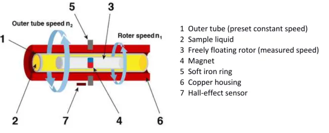
3.3.3 Stabinger Viscosimeter principle

Relatively new model, it has its origins in the year 2000, carrying out innovations such as the possibility of combining the accuracy of kinematic viscosity in a wide measuring range with just 2,5mL sample. The main elements of this device are two concentric tubes, each one with a roter speed. The outer one provides the driving force, this outer speed is constant, and the speed of the inner one is lower and it includes a magnet on it.

1 Outer tube (preset constant speed) 2 Sample liquid

3 Freely floating rotor (measured speed) 4 Magnet

5 Soft iron ring 6 Copper housing 7 Hall-effect sensor

Figure 33: Stabinger Viscometer principle.

A temperature control is carried out at the outer tube to keep the sample at the desired temperature. The second tube is submerged into the sample, but it is lighter than the sample, and it floats freely in the fluid sample. The centrifugal forces are the ones which keep the internal tube centered respecting to the outer tube. [13]

For measuring the viscosity, the magnet speed must be measure. An eddy current field is produced with an exact speed. With this way, it is possible to measure the dynamic viscosity, µ, if the two roter speeds,the outer tube speed,2 , and the roter speed 2₉ are related through this equation:

1

2 $ 2

Figure 34: Dynamic viscosity

The speed of the inner tube is measured, when the equilibrium rotor speed is reached the viscosity can be assessed. The equilibrium occurs between the driving torque MD of the rotor and the

retarding torque MR of the rotor.

MD= MR

M_D= K₁∙ μ ∙₍n₂− n₁₎

Figure 36: Driving torque of the rotor

MR= K2∙n1

Figure 37: Retarding torque of the rotor.

μ= K

(

)

Figure 38: Stabinger Viscometer principle.

The kinematic viscosity can also be estimated thanks that the device has incorporated a U-tube for measuring the density.

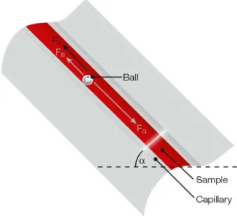
3.3.4 Rolling/ Falling ball principle

[9] As the first method explained, the gravity is also the driving force for this principle. A selected ball rolls through a tube filled with the sample, when this horizontal position is inclined at a defined angle. The angle is defined by the user, on that way, the influence of the gravity can be selected, but avoiding very speed angle that can cause turbulent flow.

The ball rolls through the tube, through a known distance. The time that the ball needs to travel that distance is measured for the subsequent obtaining of the viscosity. In that case, the fluid and the density of the ball must be known.

Depends on the inclination angle, the viscometer can be called rolling, if the angle is between 10º -80º or falling viscometer if the angle is 80º or bigger. The most common viscometer is to use a ball as a falling element, but also rods or needles can be used. Bubbles are another alternative of this principle, registering the rising time of an air bubble in the sample over a defined distance.

F_G … Effective component of gravity F_B … Effective component of buoyancy

F_V … Viscous force

The viscous force is opposite to the gravitational force, so the stronger the viscous force is, the slower the ball rolls.

=

∙ 3 $ 4 ∙

Figure 40: Dynamic viscosity. Rolling/Falling ball principle.

: ball density : sample density : ball rolling time : proportionality constant.

3.4 The Flow Behavior of Water under Pressure

The water has an anomalous behavior at +4ºC, in that point, the density has its maximum. This behavior can also be observed under pressure.

Figure 41: Water maximum density [14]

For temperatures higher than 32°C the water behaves like the other liquids and its viscosity increases while increasing the pressure, but for temperatures below 32°C and pressures less than 20MPa, the viscosity of water decreases with increasing pressure.The reason is that the structure of the three-dimensional network of hydrogen bridges is destroyed. This network is rather stronger than the structures of other low-molecular liquids.

3.5 Density

The density of a material is defined as its mass per unit volume. It is, essentially, a measurement of how tightly matter is crammed together. The principle of density was discovered by the greek scientist Archimedes.

To calculate the density (usually represented by the greek letter "ρ") of an object, take the mass (m) and divide by the volume (v):

: ;

Figure 42: Density

4. Material and methods

4.1 Capillary viscometer

[11]The viscosity measurement of Newtonian fluids can be most precisely determined using a capillary viscometer. This type of viscometer consists of measuring the time that a defined quantity of fluid needs for flowing by gravity along a given distance. The fluid arise the known distance through a capillary which length and diameter muss be known.

Thanks to the advances in the industrial production of this type of devices, this kind of method is perfectly calibrated, resulting in a reliable procedure.

The measurement of the time was realized with a stopwatch, but for minimize subjective errors, it is better to use an automatic system which was created at the stars of 1970´s.

Nowadays the capillary viscometers are essential for the control and quality for precise viscosity measurements along all over the world of Newtonian fluids in industries such as pharmaceutical or food ones.

The kinematic viscosity of liquids, , can be calculated with the instrument constant ,K, and the time, t.

The viscometer used is a viscometer with suspending ball-level which constant K was determinate by using comparative measurements with reference viscometers, this viscometer is valid for liquids with a surface tension of 20 to 30 mN/m and an acceleration of the fall of 9.8105 m/s2

Type and capillary number: 501 01/0a, which K= 0,005001 <mm_>>?

The relative uncertainly of the mentioned numerical value of K comes to 0.65% at a confidence level of 95%. It is important to check the viscometer regularly, especially, when liquids that corrode glass are being used or if the glass blowing must be repaired. It is necessary a new determination of the instrument constant.

To minimize the error, five time measurements are realized at each temperature. Then the viscosity is calculated.

The capillary viscometer consist on 3 main tubes, the one with the bigger diameter is the one through which the fluid is introduced. Another one, the measured is realized. This contains the capillary through which the fluid arise the measurement section, and the last tube is the one used for making vacuum. Furthermore, the capillary viscometer needs a device to keep it in vertical position, this device with the capillary viscometer are introduced in a cooling bath to change the temperature for doing different experiments and do the study of viscosity dependency with the temperature.

∙

First of all the desired fluid is introduced through the tube. It is necessary a known amount of fluid, so that is why in that tube there are two lines between the ones the fluid’s level must be. Once the fluid level is get, the fluid must go up through the capillary until arise the measurement area. The measurement area consist on a limited known volume by two lines, and the viscosity will be calculated according to the time the fluid spend on going from the top line to the down line. It is necessary to put a suction cup on the measurement tube to get the fluid go up while the vacuum tube is completely covered to not allow the air go into and avoiding bubbles.

Before starting the experiments, it is necessary to perform the calibration. For the calibration is necessary to compare the results obtained with the capillary viscometer and those found in the bibliography. The easiest fluid used for the calibration is the distilled water, because is one of the most studied fluids. Once it is verified that the bibliography dates coincide with the ones obtained with the experiments, it is possible to start with the measurements of the others fluids.

Figure 44: Capillary viscometer

4.2 Rotative viscometer

[15] The most suitable viscometer to measure non-Newtonian liquids are the cone-plate viscometers, although they can also be used for measurements of Newtonian fluids.

In this case, the viscometer used is the MCR 301 (Modular Compact Rheometers).

The temperature control is carried out directly in the apparatus since the viscometer is connected to a software that allows us to choose the temperature of measurement.

The speed of deformation is identical throughout the sample as long as all the extreme effects are minimized. It allows to modify, in a controlled way, the tangential deformation speed by varying the angular velocity and the time that each of them is operating. The speed setting and the reading of the corresponding values must be made without stopping the rotation.

This viscometer has a fixed plate and a rotating cone, which forms an angle with the fixed plate. The sample (with the different concentrations) is placed between them and the cone rotates on its axis to subject the sample to shear.

In this model of viscometer, the distance between the plate and the cone cannot be selected, so there will be a limit of viscosity measurement.

When the cone rotates with a given angular velocity, the sample exerts a moment on it, which is measured. [17]

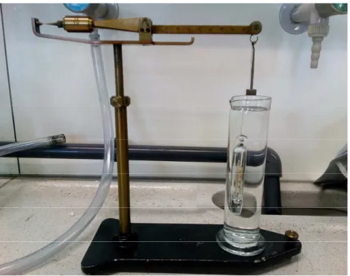
4.3 Gravitatory

This kind of viscometer are also called “falling-ball viscometer”. The operating principle consist on measured the time that a ball takes to move through a sample-filled tube. The tube is filled with the fluid from which you want to know the viscosity and the ball rolls along the tube when the horizontal position is changed to an angle of 30°. The time reading is done manually by the operator and the time measurements are collected for a subsequent calculation of the dynamical viscosity through the following equation:

3p,T4 K3p,T4∙∆t3p,T4 ∙ E 3p,T4 $ 3p,T4F ∙ 1000

Figure 47: Dynamic viscosity. Gavimetric viscometer.

The K, depends on the apparatus and represents the whole resistance of the ball in its movement to be worked against.

3p,T4

H3I4 ∙ J 3K4

_H

Figure 48: Resistance of the ball in its movement to be worked against

B is the compression of the ball and the elastic expansion of the tube under pressure.

C represents the influence of the temperature. C0 corresponds to the reference point at ambient pressure.

J 3K4

3K4

1000M

$

3K4N∙∆t 3K4

Figure 49: Influence of temperature at ambient pressure. Gavimetric viscometer.

L

3K4

∆t 3K4:

L

:

The high pressure pump is connected by one side to a valve through which the desired liquid is introduced with a syringe. To the other side, it is connected the rest of the device.

Next to the pump there is a valve, which is connected to the pressure gauge. The indicated pressure by the gauge is supposed to be the same in the whole device. After this pressure gauge there is another valve connected to a fitting, in this case it is just a union, which allows the union between the flexible capillary and the viscometer.

The viscometer is placed to the left of the capillary, which has one valve on each side and 4 sensors along it. The viscometer tube is isolated from the environment by a glass cylinder connected to a cooling bath for controlling the desired temperature and to do the measurements at different temperatures.

Figure 50: gravitatory viscometer

Figure 53: Viscometer for change the angle

First of all, the device must be installed. Every screw of the measurement set up muss be tightened at 40NM, to assure that the valves are well screw. It is necessary to use a hand spindle press, that achieved a maximal admissible pressure of 700 Mpa. Next, it must be ensured that there is no air on the circuit. While the pump is working, it is necessary to introduce the fluid through the syringe connected by a silicon tube to the setup. This silicon tube is connected to the nearby the inlet of a manual spindle pump. The pump must be turned as many times as needed to avoid air inside the circuit. It must be done with the last left valve opened to allow the air going out. The wasted fluid is collected in a vessel.

When all the air is removed, it is possible to start with the measurements.

The leftmost valve must be closed before starting the measurements. It is necessary for arising the desired pressure when we want to work with high pressure. The pressure is raised when the leftmost valve is closed and the air is compressed with the pump. The valve of the right, which connects the viscometer to the capillary must be open.

Furthermore, before starting the measurement, it is essential to check that all the sensors are working correctly. A metal rod is introduced along the viscometer tube. A software response should be seen each time the rod goes through each sensor, which means that all the sensors work correctly.

The initial viscometer position is the horizontal one, but it is necessary that the tube takes a positive angle configuration whereby the ball will be placed at the left edge of the tube. As soon as the solution is in rest, the measurements can being performed. Later, the apparatus should be inclined to the wished angle to perform the experiment.

The calculation of viscosity is done by knowing the time it takes a ball to go from one sensor to another. There are 4 sensors, but the time measured is the one between two of them, always the sensor number one, which is the reference one and one of the other three. In this case, the second sensor selected was the 4th one, which is the one furthest from the reference.

The high pressure measurements were just realized to calibrate the viscometer because for the rest of the experiments the pressure used was the atmosphereice one. For the calibration, the used fluid was distilled water, making comparisons between the values obtained with the gravitatory viscometer and the bibliography data. Ten measurements must be accomplished after the deaeration of the circuit. To assure that the internal fluid of the tube is in rest, at least 10s must pass between the performances of two consecutive measurements.

4.4 Densimeter

Mohr-Westphal balance is a balance of unequal arms that is used for the determination of liquid densities.

[2]The operating principle is the Archimedes ones, “Any object, wholly or partially immersed in a fluid, is buoyed up by a force equal to the weight of the fluid displaced by the object”. Therefore, the density could be calculated knowing the Buoyant force, E, which depends on the viscosity, , on the volume of the submerged body, V, and the gravity, g. This Buoyant force is equal to the Friction force,O

,

P $O

Figure 55: Archimede´s principle

P

∙ Q ∙ R

Figure 56: Buoyant force

O

∙ S ∙ R

Mohr-Westphal hydrodynamic balance is a balance used for the determination of liquid viscosity with its accessories : [18] a glass beaker, thermometer, balance beam, transverse notch scale (balance bar equipped with 9 positions for counter weight pieces), height variable support rod, stationary counterweight, balance indicator scale, weights and the levelling foot.

The height variable rod is screw to the support formed by the horizontal alignment screws, then the transverse notch scale is supported by the rod, and at the end of the transverse notch the thermometer is hang with a wire and introduced in the glass beaker filled with the desired fluid.

Once the different parts are put together, it is necessary to perform the calibration.

For the calibration, the used fluid is distilled water. This kind of densimeter must be calibrated each time it is used. It should be used on a horizontal surface and then the glass beaker is filled with distilled water. The 1g weight is hanging at the far right of the transverse notch and it has to be matched in horizontal position the end of the rod with the transverse notch scale by moving the screw located at the leveling foot, then the instrument is calibrated.

Figure 58: weighs

The glass beaker is filled with the fluid of which it is want to know its density. Since this moment, the weighing scales must be balanced with the weights. Four weights are provided. Each one indicates a position. It is possible to do the measurements until 3 decimals.

Application of Mohr-Westphal Balance to Rapid Calibration of Wide Range Density-Gradient Columns

5. Results

5.1 Ball viscometer calibration

The table 2 shows the data obtained during the calibration with distilled water of the Ball viscometer, at different pressures.

Table 2: Ball viscometer calibration

Pressure [bar] 1 500 1000 1500 2000

Average [sec] 4,21371 4,599215 4,419805 4,461981 4,441181 B(p) 28,94595946 29,0973457 29,2490354 29,4007251 29,5524147

K 3,47058E-08 3,4887E-08 3,5069E-08 3,5251E-08 3,5433E-08 ρF/kg/m³ 998,2450281 1019,78362 1039,51414 1057,56943 1074,12746 ρS/kg/m³ 7849,992646 7852,51663 7855,04568 7857,57473 7860,10378 ηF(20°C) /mPas 1,002 1,09634013 1,05639944 1,06956893 1,06786796

ηF,Literatur(20°C)

/mPas

1,002 1,08 0,989 1,023 1,086

The figure shows the differeces between the values of the bibliography and the ones obtained with the Ball viscometer at different temperatures.

Figure 62: high pressure viscosity

High presure viscosity

0,98 1 1,02 1,04 1,06 1,08 1,1 1,12

0 500 1000 1500 2000 2500

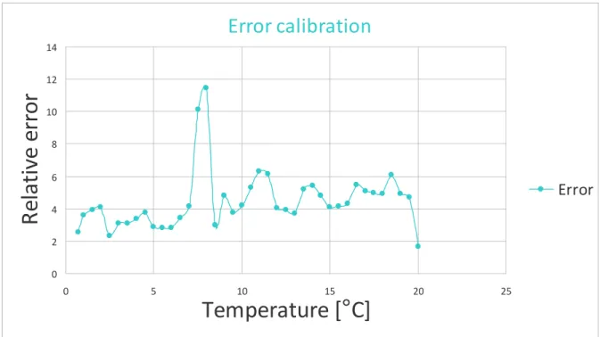
5.2 Capillary viscometer calibration

For start doing the needed measurements, the device should be calibrated. The table 3 shows the values obtained during the use of distilled water as the fluid for the capillary viscometer.

The measurements are done every 0.5°C to have a wide range of temperatures to compare properly the values obtained with the ones of the bibliography. Five viscosity measurements are done at each temperature and then the media value is the one used for obtained the viscosity. The more repetitions are performed the greater the accuracy of the measurements.

The viscosity has an inverse proportional dependence with the temperature, at the figure 64 it is possible to see that while the temperature is decreasing, the viscosity values in increases, this is because the fluid becomes more viscous and takes longer to fall through the capillary, and the viscosity is directly proportional to the time.

This tendency is observed in most of the temperatures, except at 18.5°C, 8°C and 7.5°C. In those three cases, the viscosity value instead of increase with the temperature decrease, it can be cause because of a bad control temperature or maybe time measurements errors. In those three cases also the relative error is bigger than in the rest of the temperatures. Those values are considered outliers.

Figure 63: The relative error at different temperatures

The average error is 4.45%, it was calculated taking into account the bibliography values and the ones obtained with the capillary viscometer which is an acceptable error for continue with the experiments. The standard deviation is 1.79.

Error calibration

0 2 4 6 8 10 12 14

0 5 10 15 20 25

Temperature [°C]

R

e

la

ti

ve

e

rr

o

r

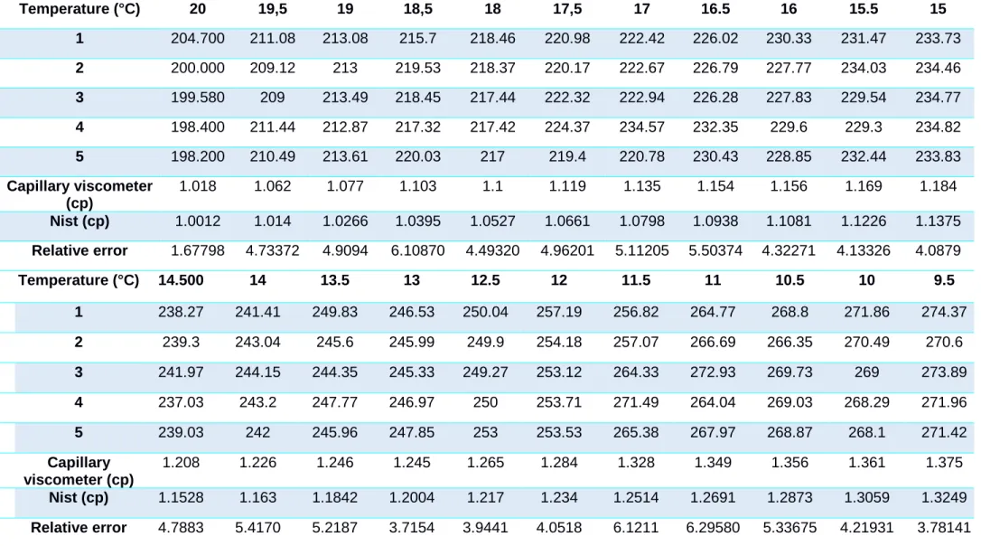
Table 3: Water viscosity (calibration)

Temperature (°C) 20 19,5 19 18,5 18 17,5 17 16.5 16 15.5 15

1 204.700 211.08 213.08 215.7 218.46 220.98 222.42 226.02 230.33 231.47 233.73

2 200.000 209.12 213 219.53 218.37 220.17 222.67 226.79 227.77 234.03 234.46

3 199.580 209 213.49 218.45 217.44 222.32 222.94 226.28 227.83 229.54 234.77

4 198.400 211.44 212.87 217.32 217.42 224.37 234.57 232.35 229.6 229.3 234.82

5 198.200 210.49 213.61 220.03 217 219.4 220.78 230.43 228.85 232.44 233.83

Capillary viscometer (cp)

1.018 1.062 1.077 1.103 1.1 1.119 1.135 1.154 1.156 1.169 1.184

Nist (cp) 1.0012 1.014 1.0266 1.0395 1.0527 1.0661 1.0798 1.0938 1.1081 1.1226 1.1375

Relative error 1.67798 4.73372 4.9094 6.10870 4.49320 4.96201 5.11205 5.50374 4.32271 4.13326 4.0879

Temperature (°C) 14.500 14 13.5 13 12.5 12 11.5 11 10.5 10 9.5

1 238.27 241.41 249.83 246.53 250.04 257.19 256.82 264.77 268.8 271.86 274.37

2 239.3 243.04 245.6 245.99 249.9 254.18 257.07 266.69 266.35 270.49 270.6

3 241.97 244.15 244.35 245.33 249.27 253.12 264.33 272.93 269.73 269 273.89

4 237.03 243.2 247.77 246.97 250 253.71 271.49 264.04 269.03 268.29 271.96

5 239.03 242 245.96 247.85 253 253.53 265.38 267.97 268.87 268.1 271.42

Capillary viscometer (cp)

1.208 1.226 1.246 1.245 1.265 1.284 1.328 1.349 1.356 1.361 1.375

Nist (cp) 1.1528 1.163 1.1842 1.2004 1.217 1.234 1.2514 1.2691 1.2873 1.3059 1.3249

Temperature (°C) 9 8.5 8 7.5 7 6.5 6 5.5 5 4.5 4

1 275.82 279.49 304.59 311.07 294.81 298.5 298.84 303.62 309.6 316.36 320.74

2 279.53 278.27 308.03 305.6 295.18 296.82 300.02 305.33 310.42 314.03 323.21

3 278.17 278.37 302.17 309.56 294.69 296.81 299.99 304.94 309.23 323.73 321.58

4 276.33 278.93 305.09 303.77 294 296.86 300.57 304.21 308.99 315.33 319.87

5 276 276.57 304.96 303.59 293 296 300 304.5 309 320.19

Capilary viscometer (cp)

1.399 1.405 1.539 1.548 1.486 1.499 1.513 1.537 1.562 1.601 1.62

Nist (cp) 1.3344 1.3643 1.3847 1.4056 1.427 1.449 1.4714 1.4945 1.5181 1.5424 1.5672

Relative error 4.8411 2.98321 11.1432 10.130 4.1345 3.45065 2.82723 2.84376 2.89177 3.79927 3.3690

Temperature (°C) 3.5 3 2.5 2 1.5 1 0.7

1 324.23 331.59 336.67 340.13 353.19 353.59 357.2

2 325.69 331.01 335.69 346.61 348.34 354.89 358.07

3 323.5 330.92 335.11 346.34 351.19 355.34 358.72

4 325.97 329 335 348 349.79 358.01

5 327.44 331.1 346.69 351.96 358.65

Capilary viscometer (cp)

1.642 1.669 1.693 1.742 1.769 1.793 1.806

Nist (cp) 1.5927 1.6189 1.6548 1.6734 1.7017 1.7309 2

The figure 64 shows the differences between the experimental viscosity and bibliography viscosity of water during the calibration of the capillary viscometer.

Figure 64: Differences between experimental and bibliography viscosity

Calibration

0,800 1,000 1,200 1,400 1,600 1,800 2,000

0 5 10 15 20 25

Temperature (

°

C)

V

is

co

si

ty

(

cp

)

Experimental viscosity

5.3 Viscosity/density measurements: solution 5.7% sucrose mass

The following table shows the viscosity measurements realized at different temperature with a mass sucrose concentration of 5.7%.

Table 4: 5.70% w/w sucrose

Temperature (°C) 20 19 18 17 16 15 14 13 12 11 10

1 237.97 242.68 247.77 258.63 264.78 271.66 274.53 285.62 294.49 310.47 316.93

2 236.75 240.62 247.56 256.24 262.83 269.62 277.72 285.34 294.43 307.24 319.86

3 235.99 241.7 246.09 254.23 259.82 268.86 277.73 283.82 292.7 307.61 316.65

4 238.23 244.27 245.52 256.57 259.81 268.55 276.78 292.59 289.37 301.21 311.89

5 235.57 246.91 246.27 256.33 262.72 270.77 277.32 288.73 291.25 302.03 309.84

Capilary viscometer (cp)

1.186 1.218 1.234 1.283 1.311 1.35 1.385 1.437 1.463 1.529 1.576

Temperature (°C) 9 8 7 6 5 4 3 2 1

1 320.57 337.53 341.03 355.17 364.54 375.06 387.67 398.51 414.29

2 320.63 336.26 340.23 351.98 363.94 374.24 386.15 398.55 417.67

3 320.67 335.71 339.1 350.86 363.91 372.89 386.65 400.03 417.04

4 319.55 334.16 340.92 351.19 362.57 373.37 385.49 399.12 416.3

5 335.32 338.97 351.3 370.5 373.77 385.8 402.61 415.9

Capilary viscometer (cp)

The next figure show the variation of viscosity with temperature of a solution with 3.7% of mass sucrose.

Figure 55: Viscosity solution 3.7% sucrose mass

The following table shows the density measurements realized at different temperatures with a mass sucrose concentration of 5.7%.

Viscosity solution 3.7% sugar

y = -0,0463x + 2,0567

0 0,5 1 1,5 2 2,5

0 5 10 15 20 25

Temperature (

°

C)

V

is

co

si

ty

(

cp

)

Viscosity

Lineal (Viscosity)

Temperature (°C) 20 19 18 17 16 15 14 13 12 11 10

Density (Kg/m3_{) 1.023 1.023 1.023 1.023 1.023 1.023 1.023 1.023 1.023 1.023 1.023}

Table 4: 5.7% w/w sucrose density.

Temperature (°C) 9 8 7 6 5 4 3 2 1 0.5

5.4 Viscosity/density measurements: solution 5.7% sucrose mass

The following table shows the viscosity measurements realized at different temperature with a mass sucrose concentration of 30%.

Temperature (°C) 20 19 18 17 16 15 14 13 12 11 10

1 456.63 467.22 492.56 520.55 528.88 531.99 585.47 605 668.87 656.51 655.34

2 464.67 466.23 480.41 513.07 524.37 532.09 577.27 590.69 666.43 644.63 669.88

3 454.91 467 479 518.43 521.99 530.63 581.59 597.27 665.37 574 649.12

4 454.06 467.9 486.96 511.36 519.14 531.33 577.81 659.68 663.12 647.52 648.13

5 456.83 478.91 511.03 518.35 578.59 659.43 699.6 647.63

Capilary viscometer (cp)

2.285 2.334 2.416 2.572 2.61 2.655 2.897 3.108 3.325 3.218 3.266

Table 6: Viscosity solution 30% w/w sucrose.

Temperature (°C) 9 8 7 6 5 4 3 2 1.4

1 665.53 687.08 713.59 710.7 734.77 753.87 807.72 823.12 861.33

2 672.54 686.08 713.67 710.89 732.59 754.73 803.93 818.46 867

3 668.17 686.79 765.36 710.42 737.57 753.48 799.84 799.38 868

4 670.99 747.27 729.64 794.83 784.16 857.62

5 668.23 690.94 729.23 799.75 798.79 860

Capilary viscometer (cp)

3.341 3.428 3.625 3.548 3.658 3.764 4 4.017 4.307

Figure 66: Viscosity solution 30% sucrose mass

The following table shows the density measurements realized at different temperatures with a mass sucrose concentration of 30%.

Table 7: 30% w/w sucrose density.

Temperature [°C] 20 19 18 17 16 15 14 13 12 11 10

Density [Kg/m3] 1.108 1.108 1.108 1.108 1.108 1.108 1.108 1.108 1.108 1.108 1.108

Temperature [°C] 9 8 7 6 5 4 3 2 1 0.5

Density [Kg/m3] 1.108 1.108 1.108 1.108 1.108 1.108 1.108 1.108 1.108 1.108

Viscosity Solution 30%sugar

y = -0,1002x + 4,2728

0 0,5 1 1,5 2 2,5 3 3,5 4 4,5 5

0 5 10 15 20 25

Temperature (

°

C)

V

is

co

si

ty

(

cp

)

Viscosity

Lineal (Viscosity)

5.5 Viscosity/density measurements: solution 45% sucrose mass

The following table shows the viscosity measurements realized at different temperatures with a mass sucrose concentration of 45%.

Table 8: Viscosity solution 45% w/w sucrose.

Temperature [°C] 20 19 18 17 16 15 14 13 12 11 10

1 1550.07 1361.24 1663.65 1772.17 1848.73 1886.46 1991.87 2144.27 2010.67 2325 2443

2 1545.3 1519.71 1664.65 2009.22 1799.64 1896.21 1988.56 2147.31 1978.52 2325.6

3 1539.47 1286.36 1648.98 1927.97 1809.13 1900.71 1941.13 2150 1967.89

4 1629.89 1893.55 2145.69

5 1420 1601.4 2042.59

Capilary viscometer (cp)

7.668 7.646 8.277 9.875 9.075 9.451 9.847 10.711 9.906 11.599 12.186

The following table shows the density measurements realized at different temperatures with a mass sucrose concentration of 45%.

Table 9: 45% w/w sucrose density.

Temperature [°C]

20°C 19 18 17 16 15 14 13 12 11 10

Density [Kg/m3]

The next figure show the variation of viscosity with temperature of a solution with 45% of mass sucrose.

Figure 67: Viscosity solution 45% sucrose mass

5.6 Density

The next figure shows the density of different solutions at different concentration and temperatures.

Figure 68: Experimental density

Viscosity solution 45% sugar

0 2 4 6 8 10 12 14

0 5 10 15 20 25

Temperature [

°

C]

V

is

ci

si

ty

[

cp

]

45% sugar

Lineal (45% sugar)

Density

0 5 10 15 20 25

Temperature [

°

C]

5.7 Rotative viscometer. MCR 301

The figure 69 and the figure 70 show the viscosity measurement realized at 20°C and 15°C respectively with the rotative viscometer MCR 301 of a solution with 45% in sucrose mass.

Figure 69: Viscosity at 20°C.Rotative viscometer

Figure 70: Viscosity at 15°C.Rotative viscometer

0 10 20 30 40 50 60 70 80 90 100 0 2 4 6 8 10 12 14 16

20°C

Viscosity

Shear Stress [Pa]

µ

[

m

P

a

·s

]

0 20 40 60 80 100 120

0 2 4 6 8 10 12 14 16 18

15°C

Viscosity

Shear Stress [Pa]

5.8 Rotative viscometer. MCR302

The figure 71 and the figure 72 show the relation between the shear stress and the shear rate at 20°C and 15°c respectively realized with the rotative viscometer MCR 302 at Busan University of a solution with 45% in sucrose mass.

Figure 71: Relation between shear stress and rate at 20ºC. MCR 302 [19]

Figure 72: Relation between shear stress and rate at 15ºC. MCR 302 [19]

0 2 4 6 8 10 12

0 100 200 300 400 500 600 700 800 900 1000

S h e a r-S tr e ss [P a ] Shear-rate [1/s]

20 °C

0 100 200 300 400 500 600 700

The next figure shows the viscosity differences between the results obtained with the capillary viscometer and the rotative viscometer MCR 302.

Figure 73: Viscosities calculated with rotative viscometer MCR 302 [19]

To know more about the obtained data, see Annexes.

5 7 9 11

0 100 200 300 400 500 600 700

V

isco

si

ty

[m

P

a

.s]

Shear-rate [1/s]

Comparing viscosities

15°C

Capillary Viscosimeter [15°C] 20°C

6. Discussion

It has been checked that the most significant thing for taking into account is the dependency of the viscosity with the temperature, that’s why the project is focused on this parameter and not on the pressure.It is showed at table 2. In most of the fluids, the viscosity increases with increasing pressure, but the influence of pressure compared with the temperature influence is insignificant, the reason is that liquids are almost non-compressible at low or medium pressures; a change of 0.1MP to 30 MP has the same effect than increase the temperature 1°C. In the table 2, it is possible to see the pressure influence on viscosity, an increase from 1 to 2000bar only affects 0,067 to the value of the viscosity. It was checked with a falling ball viscometer.

The study of the relative error at the figure 63(capillary viscometer calibration) shows that the error decrease at lower temperatures, being around 4 and 6 from 20°C to 9°C and an error from 4 to 2,31 between 9 and 1 °C ( under the average error), which can mean that at lower temperatures the quality of the results with the capillary viscometer is better than at high temperatures. The average error has a value of 4.45%, is an acceptable error to perform the experiments with the rest of samples and get good results.

Comparing all the viscosities at figure 74, it is seen that the tendency in all is the decrease of the viscosity when the temperature increases.

When the sucrose concentration is low, the viscosity difference with the pure water is very small, the difference increases as the concentration of sucrose increases.

The linear tendency of the viscosity is clear at low concentrations, but at concentrations of 45% of sucrose the variation of the viscosity with the temperature is not as linear as in the other cases, this can be due to the high concentrations of sucrose. The solution presents certain non-Newtonian behavior, and the measurements with the capillary viscometer are not as correct as in the other cases.

Figure 74: Experimental viscosities

Viscosity

0 5 10 15 20 25

Temperature [

°

C]

After studying the density of the samples, small variations of the density with respect to the changes in temperature have been observed but there is a great difference in the densities of the samples at different concentrations.All the viscosities are collected at the figure 68.

The density increases as the sucrose concentration increases, but the difference between the density of the sample with the highest concentration of sucrose and water is only 0.206Z[

:\ in density. Thus, the sucrose concentration does not significantly affects the density variation.

Due to the 45% solution the sucrose concentration is so high and that the capillary viscometer is just valid for Newtonians fluids, it must be assured that the solution has this characteristic. A rotational viscometer plate-cone MCR301 was used to check this. At Figure 69 and at figure 70, we can see that there are not viscosity variations with respect to the changes of shear stress, so, that means that our fluid is Newtonian.

The first check was not made with the rotational viscometer most appropriate for our type of fluid, so a new check was made to ensure the behavior of the fluid, the selected one was MCR302 and the experiments were realized at Busan (Korea). See results displayed in section 5.8.

The selected temperatures were 20°C and 15°C, the figures 71 and 72. There is a slight variation of the viscosity with the shear-stress, because this variation is not very significant. Nevertheless, the sample can still be rationed as a Newtonian fluid.

There are some differences between the viscosity obtained with the capillary viscometer and the ones obtained with the rotational MCR 301. The ones measured with the rotational are 30% bigger. It can be due to our fluid is not very viscous. The viscosity of the sample could be out of the lower limit of acceptability for those measurement systems. Representing the shear stress in the y-axis and the deformation speed in the x-axis, a slight tendency to shear-thinning is seen from deformation rates above 8000 1 / s. It is possible, however, that the reduction in viscosity is due to measurement errors at high deformation rates.

It is possible that the use of the capillary viscometer results in a systematic error at such high concentrations, but this error is very small because the results fit well with the rheometer in the strain rate range presented in figure 73.

The capillary viscometer is based on an approximation of a Hagen Pouiselle flow to determine analytically the flux with viscosity as the only unknown in the equation. As the volume is known, it is enough to measure the time that the fluid needs to move from one point to another. When one looks at the assumptions for that flow of Hagen Pousille, the first thing one sees is that the equation is based on Navier-Stokes equations, which assume a Newtonian flow. However, the fluid appears to have a tendency to dilatant fluid typical of suspensions with high concentration. As a consequence, this equation, in the most rigorous of the senses, should not be applied since the viscous effort is not completely linear with the rate of deformation.

7. Conclusion and outlook

For future studies on the formation of gas hydrates in juices have been made density and viscosity measurements of a water solution with sucrose at different concentrations to simulate the behavior of the juices. Both properties have been measured at different temperatures since the formation of gas hydrates these pass through different phases.

The density measurement was carried out with a traditional densimeter, Mohr-Westphal balance. For the measurement of viscosity, the experiments were started with a gravitational viscosimeter, but when seeing that there was no great dependence of the viscosity with the pressure was proceeded to calculate with a capillary densimeter

After comparing the results obtained with those of the literature, an error of 4% was obtained, so the methods used are appropriate to obtain the viscosity measurements.

After comparing the results obtained with those in the literature, an error of 4% was obtained, so the methods used are appropriate to obtain viscosity measurements, also at high concentrations of 45% by mass of sucrose. To ensure that the solution with 45% sucrose had a Newtonian behavior and therefore the capillary viscometer can be used, measurements were made at various temperatures with rotational viscometers: MCR301 and MCR302.

According to the density, it has been observed that the temperature changes do not affect this variable very much but the changes in the concentration affects.

8. Annexes

The tables 10 and 11 show the results obtained with a rotative viscometer MCR 301 at 20°C and 15°C of a solution with 45% of sucrose mass.

Table 10: Measurement with rotative viscometer MCR301 at 15°C.

Meas. Pts.

Shear Rate Shear Stress Viscosity Torque

[1/s] [Pa] [mPa·s] [µNm]

1 6.43 0.1 15.5 3.27

2 8.76 0.115 13.1 3.77

3 10.5 0.133 12.6 4.34

4 12.2 0.153 12.5 4.99

5 13.9 0.176 12.6 5.75

6 16.2 0.202 12.5 6.62

7 18.6 0.233 12.5 7.62

8 21.5 0.268 12.5 8.78

9 24.6 0.309 12.5 10.1

10 28.4 0.356 12.5 11.6

11 32.8 0.409 12.5 13.4

12 37.7 0.471 12.5 15.4

13 43.5 0.543 12.5 17.8

14 50 0.625 12.5 20.5

15 57.7 0.72 12.5 23.5

16 66.5 0.829 12.5 27.1

17 76.5 0.954 12.5 31.2

18 88.1 1.1 12.5 35.9

19 102 1.26 12.5 41.4

20 117 1.46 12.4 47.7

21 135 1.68 12.4 54.9

22 155 1.93 12.4 63.2

23 179 2.22 12.4 72.7

24 206 2.56 12.4 83.7

25 238 2.95 12.4 96.4

26 274 3.39 12.4 111

27 315 3.91 12.4 128

28 363 4.5 12.4 147

29 418 5.18 12.4 169

30 482 5.96 12.4 195

31 555 6.87 12.4 225

32 638 7.91 12.4 259

33 735 9.1 12.4 298

34 846 10.5 12.4 343

35 974 12.1 12.4 395