Generative Models for Video Analysis and 3D Range Data Applications

(1)

Chapter 5 A Polynomial Fiber Description of

Motion for Video Mosaicing

This chapter is about two topics. First,given a video sequence,we introduce a Bayesian framework,where background and moving objects are segmented into lay-ers. The model that describes the different layer evolutions in a sequence of images uses the results of a multi-frame optical flow estimation (MFOFE); we present a new technique based on the fact that each pixel in the frame of reference produces a trajectory in the mosaic absolute coordinate system. The second topic is video sum-marization. A general moisaicing method is presented for describing the background and the trajectories of moving objects in a sequence of frames. Combining layer segmentation and mosaicing,we show different manners of encoding and visualizing temporal information,where the key point is the selection of a certain object in the images as reference in the evolution.

5.1 Introduction

S

ummarizing the contents of a video into a single image is a very useful tool for video indexing and compression purposes [46, 102]. Indeed, browsing and re-trieval by content in video data-bases are becoming a relevant ﬁeld in Computer Vision and Multimedia computing. This fact goes in accordance with the increasing developments in digital storage and data transmission. In addition to this, the wide range of applications in this framework, such as advertising, publishing, news and video clips, points out the necessity for more eﬃcient organizing techniques. In this chapter, we focus on two important subjects in this area, movement segmentation and video mosaicing as a summarization technique. These subjects make feasible a quick intuition of the evolution of higher level perceptual structures, such as scenes, short stories and panoramic view sequences [98, 93]. Algorithms for image mosaicing

(2)

118A POLYNOMIAL FIBER DESCRIPTION OF MOTION FOR VIDEO MOSAICING

sist of two main steps: registration, i.e. estimating the transformation that occurred across consecutive frames in the sequence, and mosaic construction, which implies utilizing the previously estimated transformations in conjunction with the images to be summarized. These two steps are intrinsically related. A good performance of the resulting ﬁnal mosaic is strongly dependent on the variety of techniques which are applied in both steps.

The first step,transformation estimation, is usually based on optical flow estima-tion in pairs of consecutive frames. However, when images are put in correspondence, rather than an estimation of the relative transformation between consecutive images, a estimation of the absolute transformation between each frame and a selected frame of reference is more necessary. This goes in accordance with the fact that a mosaic coordinate system has to be selected in order to locate the images of a sequence in a mosaic structure. For this reason, in this chapter, we apply the Multi Frame Optical Flow estimation (MFOFE) introduced in [45], since it provides a global estimation of images transformation respect to a previously selected frame of reference. Moreover, this technique offers a good solution to the aperture problem without assuming an a-priori restricted model of the world or of the camera motion.

The second step, mosaic’s structure construction, utilizes the world coordinate transformations to put images in correspondence, i.e., to estimate the overlapped regions that are common in the images of a sequence. The presence of moving objects in a scene gives rise to a more complex situation. In this case, background and object motions must be separated in order to obtain an accurate registration. To this end, we present a new technique where each pixel in the frame of reference produces a trajectory in the mosaic absolute coordinate system. Unlike techniques which are restricted to pairs of frames [105, 6, 88], this method performs simultaneously a global motion segmentation across all the frames. Clustering is based on the fact that similar trajectories will correspond to the same sort of motion (and camera operation). Thus, we introduce a description of these paths in terms of polynomial fibers, and a probabilistic model is developed in order to rely on a measure of similarity as well as to have a classification mechanism which extracts the possible different classes of motions.

The outline of this chapter is as follows: first, we introduce a description of the features (fibers) that are used to the analysis of the relative movements among differ-ent objects. Subsequdiffer-ently, a probablisitic model and an EM algorithm are presdiffer-ented in order to establish the settings for classification. Section 3 shows the development used for mosaic’s structure construction and the application of the information of the fibers model. Finally, the chapter is concluded with the summary and conclusions.

5.2 Motion in terms of Fiber-Like Structures

(3)

5.2. Motion in terms of Fiber-Like Structures 119

(a) (b)

Figure 5.1: (a) Description of a ﬁbre in terms of absolute coordinates; it starts in (xn

0, y0n),and,by successive applications of the corresponding absolute velocities

ωf, the points in the ﬁber (xn

f, yfn) are obtained. (b) Fiber picture in the mosaic

coordinates.

employing all the information from the sequence.

5.2.1 Settings

The starting point is to deﬁne the features that are used to the analysis of relative movements among diﬀerent objects in a sequence ofF images_{I0, . . . , IF}, where each

imageIf consists ofN pixels. LetI0 be the absolute frame of reference and (xn0, y0n)

then-th pixel in this frame, thus, (xn

f, yfn) is the resulting pixel in the fth-frame of

applying the absolute velocity vectorωfto (xn0, y0n). MFOFE allows to estimate these

absolute coordinates that correspond to this pixel in the following frames. Following the scheme in ﬁg. 5.1, we deﬁne afiber S(n) for each pixel (xn

0, yn0) in I0 as:

S(n) = [(xn0, yn0), . . . ,(xnF, yFn);v1, . . . , vF]

where each vi is a relative velocity vector obtained through the diﬀerence of the

absolute velocities which are provided by MFOFE, i.e., vf = ωf −ωf−1. In this

way, rather than analyzing point pixel structures, it turns out to be more robust the analysis of ﬁbers which are associated to each pixel in the selected frame of reference.

5.2.2 A Polynomial Surface Model

We consider the whole sequence of images as a fiber bundle. Each fiber can be described in terms of a polynomial model as follows: letS(n) be the fiber associated to then-th pixel inI0, therefore, the components of the velocity vectors can be fitted

to a polynomial of degree1_d_:

unf = a00+a10xfn+a01yfn+aij(xnf)i(yfn)j+. . .+a0d(yfn)d vfn = b00+b10xfn+b01ynf +aij(xnf)i(yfn)j+. . .+b0d(ynf)d

1_When_d_{= 0, the polynomial corresponds to a translation,}_d_{= 1 to an affine model and}_d_{= 2 to}

(4)

wherevn

f = (unf, vnf) (relative velocity) is analyzed in terms of its components, and the

coordinates in thef-thframe are represented by (xn

f, yfn)2. The number of unknown

coeﬃcients in each polynomial isr= (d+1)(₂d+2). Besides, the previous forms can be written in terms of an inner product of the following vectors:

pnf =

1, xnf, ynf, . . . ,(xnf)i(yfn)j, . . . ,(xnf)d,(ynf)d T

α = (a00, a10, a01, . . . , ad0, a0d)T

β = (b00, b10, b01, . . . , bd0, b0d)T

hence, the velocities ﬁtting can be re-written as follows:

unf = [pnf]Tα (5.1)

vnf = [pnf]Tβ (5.2)

Let Un _and _Vn _{be the column vector} _F

×1 of the velocity components in the ﬁberS(n), andPn _{a matrix} _r_×_F _{of its corresponding point [absolute] coordinates,}

therefore, eq. (5.1) and eq. (5.2) are extended in a matrix form:

Un = [Pn]Tα (5.3)

Vn = [Pn]Tβ (5.4)

whereαandβarer_×1 vectors. In the following section, we introduce a probabilistic formulation to estimate a mixture of surfaces that describe the behavior of the diﬀerent sort of movements which are present at the video sequence.

5.2.3 Probabilistic Mixture Model

Describing a fiberS(n) in terms of a set of coefficients Ω =_{α, β_} gives us a starting point to develop a probabilistic formulation. The idea behind this, is to provide a model that permits a classification of different types of fibers. These classes are related with the sort of diferent movements that are produced in the sequence. Consider eqs. (5.3) and (5.4) as the generative functions of the velocities along a fiber. Under the assumption of independent zero-mean Gaussian distributed noise in the velocity components, the likelihood function of a fiber, for a given instance of the model Ω, is3_:

P(Un, Vn|Pn,Ω) =P(Un|Pn,Ω)P(Vn|Pn,Ω) (5.5) where,

P(Un|Pn,Ω) = √ 1

2πσ2

u

exp

−₂_σ1₂ u |

Un−[Pn]Tα|2

P(Vn|Pn,Ω) = √1

2πσ2

v

exp

−₂1_σ₂ v |

Vn−[Pn]Tβ|2

2_{Recall superscript}_n_{is related to (}_xn

0, yn0) in the frame of reference

3_{This model assumes independence between the velocity components. Due to this assumption, eq.}

(5)

5.2. Motion in terms of Fiber-Like Structures 121

When different types of movement are present in an image sequence, their fiber representation leads to take into account more than one model. Consider that a fiber can be explained by a set ofQmodels_M=_{Ω1, . . . ,ΩQ}. In this case, the likelihood

function (5.5) corresponds to a probability that is conditioned to a certain sub-model Ωi,P(Un, Vn|Pn,Ωi). Therefore, the global likelihood function is:

P(Un, Vn|Pn,M) =

Q

i=1

P(Ωi)P(Un, Vn|Pn,Ωi) (5.6)

whereP(Ωi) is a prior distribution over the sub-model Ωi. Given a instance of these

sub-models, the classiﬁcation of each ﬁber in a sequence of frames is a matter of Maximum a Posteriori (MAP), Ωi = argmaxi′P(Ωi′ |Un, Vn, Pn) which is given by

the Bayes rule:

P(Ωi|Un, Vn, Pn) = P(Ωi)P(U

n_{, V}n_|_Pn_,_Ω i)

Q

i′=1P(Ωi′)P(Un, Vn|Pn,Ωi′)

(5.7)

5.2.4 EM Algorithm

The Expectation-Maximization approach is applied to this problem in order to es-timate the models that explain the different fiber categories. This is based on the maximization of a likelihood function of the set of fibers that are obtained from the image sequence. Considering the approximation of independent observations among fibers, the global likelihood function of a set of fibersS(1), . . . , S(N) (N is the number of pixels in the frame of reference I0) is written as a product of single likelihoods.

Equivalently, this maximization can be done through maximizing the log-likelihood:

L=

N

n=1

log

_Q

i=1

P(Ωi)P(Un, Vn|Pn,Ωi)

(5.8)

When assuming that each ﬁber is explained by only one sub-model Ωi, eq. (7.4) can

be written in terms of binary variableszni:

L=

N

n=1

Q

i=1

znilog{P(Ωi)P(Un, Vn|Pn,Ωi)} (5.9)

The EM algorithm consist of a two-step iterative procedure that converges to a local maximum of (7.4):

• E-step: set Rni =P(Ωi | Un, Vn, Pn) and compute the posterior expectation

of (5.9).

• M-step: for each sub-model Ωi

1. P(Ωi) =N_n₌₁Rni/N

2. αi =*N_n₌₁RniPn_[_Pn_]T+−1*N n=1RniP

(6)

3. βi =*N_n₌₁RniPn[Pn]T+

−1*

N n=1RniP

n_Vn+

4. σ−2

ui = N1 n=1Rni

N

n=1Rni|U

n

−[Pn]Tαi|2

5. σ−2

vi = N1 n=1Rni

N

n=1Rni|V

n

−[Pn]Tβi |2

These steps are iterated until a certain convergence criteria.

5.3 From video to Mosaic Representations

The previous representation of motion in terms of ﬁbers has two straight forward applications: 1) a motion clustering of the diﬀerent regions in the reference image, which is extended to all the images of the sequence, and 2) permits an estimation of the global transformation that is produced in each segmented region. This second issue allows to a priori estimate the size of the mosaic, since those transformations are computed taking as reference a common frame for all the images. Thus, the trans-lation contribution of global transformation of the ”furthest”4 _{frame will determine}

such a size.

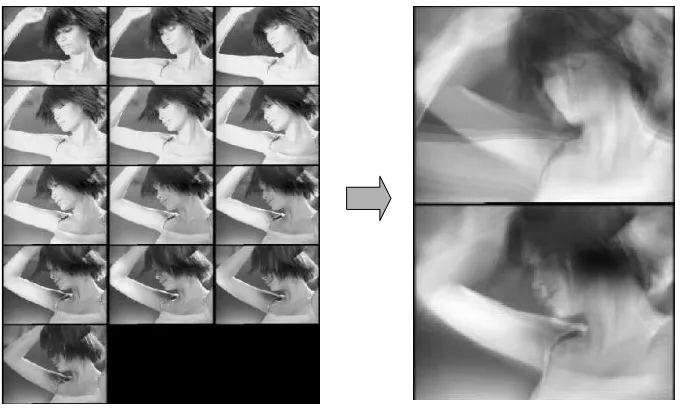
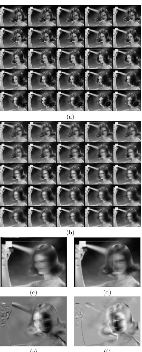
Besides, in order to build the mosaic we have to select which layer is taken as reference as well. The selection of a layer as reference will completely determine the action that is summarized in the final mosaic. For instance, fig. 5.4 (a) shows a mosaic, where the reference layer is the segmented background, and fig. 5.4 (b) is given by choosing as reference the segmented foreground. The layer selection procedure is carried out thought using the maximum a posteriori probability in eq. (5.7), which is assigned to each fiber of the sequence. In this way, a sequence of labeled images is produced, where each label indicates the ownership of each fiber to a certain layer.

Once the reference layer is selected, all the images in the sequence are put in correspondence by means of the estimation of the global transformations of each image with respect to the reference frame. This can be performed easily by fitting the optical flow in each image (separately) using: either a 1-degree polynomial function (affine model), or 2-degree polynomial (projective model). Figure 5.3 show a picture of the mentioned data structure. When images are put in correspondence, each position in such a data structure indicates those pixel that will contribute to the formation of the final mosaic. At this point, given a instance of the data structure, the final mosaic can be presented in two manners. First, when the labeling, which was obtained using the fiber analysis, is utilized, the final mosaic will only take into account those pixels that belong to the selected layer. This result is shown figures 5.4 (c) and (d), where (c) is a mosaic that takes a reference layer the background, and (d) the mosaic that only considers the segmented foreground. In these two mosaic appear black areas that indicate that the layer that has been taken as reference had no information in these regions. In (c) the black region corresponds to a zone where the tree-layer was present in the whole sequence. The second option is to consider all the pixels in the images;

(7)

5.4. Conclusions and future work 123

Figure 5.2: Three frames from a sequence of 25.

(a) (b)

Figure 5.3: Scheme of the data structure.

this result is shown in fig. 5.4 (a) and (b). It is worth it to comment that the pixel that appears in the final mosaic (for each position in the data structure) is obtained is these examples by a median computation. Our purpose is to point out that once the introduced data structure is computed, the different resulting mosaics come from this common structure. The only thing that differs is whether a labeling mask is used or not, and the selected operation, such as median or average, is employed in order to determine which pixel from the frames, that contribute to a certain location in the data structure, is shown in that final mosaic.

In ﬁgure 5.2 we show three frames of the video sequence that has been used for these examples. Finally, in ﬁgure 5.5 we show a mosaic, where the reference layer is he background, which has three masks of the foreground in order to summarize the video sequence.

5.4 Conclusions and future work

(8)

(a) (b)

(c) (d)

(9)

5.4. Conclusions and future work 125

(10)

(11)

Chapter 6 Video Summarization through

Iconic Data Structures

Representing motion into a single image has been a challenge since the beginnings of Humanity (from cavern hunting paintings to modern art). Even children,when drawing their parents’ car in motion,add some oriented blurring eﬀects in order to represent time in a single picture. Such a form of compression,from a temporal sequence of images to a reduced set,is straightforwardly meaningful,since we are able to reconstruct an approximation of the original temporal sequence from our ex-perience. In this chapter,we address the video summarization problem in a Bayesian framework in order to detect and describe the underlying temporal transformation symmetries in a video sequence. Given a set of time correlated frames,we attempt to extract a reduced number of image-like data structures which are semantically meaningful and that have the ability of representing the sequence evolution. To this end,we present a generative model which involves jointly the representation and the evolution of appearance. Applying Linear Dynamical System theory to this problem, we discuss how the temporal information is encoded yielding a manner of grouping the iconic representations of the video sequence in terms of invariance. The formu-lation of this problem is driven in terms of a probabilistic approach,which aﬀords a measure of perceptual similarity taking both learned appearance and time evolution models into account. This measure provides a setting for assigning boundaries to sequence of frames.

6.1 Introduction

O

rganizing, browsing and retrieval by content in video data-bases is becoming a relevant ﬁeld in Computer Vision and Multimedia Computing. This fact goes in accordance with the increasing developments in digital storage and transmission. In addition to this, the wide range of applications in this framework,

(12)

128 VIDEO SUMMARIZATION THROUGH ICONIC DATA STRUCTURES

such as advertising, publishing, news and video clips, points out the necessity for more eﬃcient organizing techniques [30, 76].

[image:12.595.113.453.420.627.2]

In this chapter, we focus on two important subjects in this area that are video preview and summarization, and, which make feasible a quick intuition of the evolu-tion, under a low streaming cost, of higher-level perceptual structures, such as stories, scenes or pieces of news. That fact becomes relevant for low bandwidth communi-cation systems. Expressing a video sequence in terms of a few representative images permits a continuous media to beseekable. Besides, the summarizing ability of a story will depend on the specific choice ofkey-framesset. Currently, the standard approach for keyframes selection, as indicators of the content of video, is to choose certain im-ages that belong to the video sequence, which usually correspond to the beginning and the end of clips. However, considering that editors, authors and artists utilize camera operations to communicate some specific intentions, this standard key-frame selection may presents the risk of losing semantic information. Selecting solely one image of the sequence to represent its temporal evolution may lack of expressiveness in terms of summarization purposes. When more than one types of motions (due to different frequencies, velocities, etc) are involved in the sequence, more than one icon are necessary to represent it. For instance, figure 6.1 shows a sequence of images where two main types of motions are involved. On one hand, the arm is rising with a certain velocity, while, on the other, the head is turning with a different rapidity of movement.

Figure 6.1: Semantic keyframes summarization of a sequence of images.

(13)

6.2. On underlying symmetries 129

based on an application of Linear Dynamical System and Lie’s group theories, which are our support to define temporal symmetries and invariances. In this framework, the temporal information is encoded in an infinitesimal generator matrix, which de-fines different types of behaviors in the evolution of an image sequence. We use this distinct sort of contributions to give, in addition, a grouping inside the summarized representation.

The formulation of this problem is driven in terms of a probabilistic approach. Appearance representation and time evolution between consecutive frames are in-troduced in a generative model framework. First, a feature space is built through Probabilistic Principal Component Analysis (PPCA) [15], since this technique allows to codify images as points capturing the intrinsic degrees of freedom of the appear-ance, and at the same time, it yields compact description preserving semantics and perceptual similarities [106, 77, 68]. Subsequently, we present a generative dynam-ical model for the estimation of the curve’s behavior that the sequence of images describe in this subspace of principal features. Authors in [82] introduced previously this dynamical model in a neural network framework. However, we embed it into a latent variable model, providing an EM algorithm for its estimation. This fact avoids undesirable problems such as when it comes to instantiate by hand the update steps of gradient descents techniques. Furthermore, the presented latent variable model allows a conjugation of both semantic and temporal representations. This aﬀords a measure of perceptual similarity taking both learned appearance and time evolution sub models into account. Indeed, this probabilistic framework allows determining whether two consecutive images are in accordance with the learned dynamical model. This fact has an important signiﬁcance when it comes to assign some boundaries to a sequence of frames.

The outline of this chapter is as follows: ﬁrst, we introduce a review on Linear Dynamical Systems. The aim of this is to present the key points on the interpretation of the temporal appearance codiﬁcation and how this information can be extracted. Subsequently, in section 3, an appearance probabilistic framework for time symmetry estimation is introduced in terms of latent variable models. Section 4 shows the exper-imental results in order to see this framework applied to real image problems. Section 5 presents the summary and conclusions. Finally, the appendix gives a detailed ex-planation of the developed EM algorithm for the dynamical model estimation.

6.2 On underlying symmetries

Consider a sequence of frames_F=_{φ0, ..., φN}that are represented as vectors. Each

vector corresponds to an image read in lexicographic order belonging to a subset of real numbers _{S ⊂ ℜ}d_{. Since images are obtained from a temporal sequence,}

(14)

approximation order, the relation between an image φ0 and a near one transformed

φ(δθ) can be expressed as: φ(δθ)_≃(1 +δθG)φ0. So, a macroscopic transformation

T(θ) can be built in terms of concatenating inﬁnitesimal transformations, dividing the parameterθ inM parts and makingM _{→ ∞}:

φ(θ) = lim

M→∞

1 +

θ M

G

M

φ0=eθGφ0 (6.1)

Equation (6.1) is related with to the study of a trajectory near a ﬁxed point in _S described by a linear dynamical system:

˙

φ=Gφ (6.2)

The basic idea considering a trajectory in _ℜd_{, formed by a sequence of images}

F= {φ0, ..., φN}, is to understand as a video sequence with some underlying appearance

invariance. From a geometric the point of view invariance is deﬁned as follows:

Definition 6.2.1 Let_{S ⊂ ℜ}d _{be a set, then}

S is said to beinvariantunder the vector

fieldφ˙=T(φ)if for anyφ0∈ S we have φ(θ, φ0)∈ S for allθ∈ ℜ.

Furthermore, we can see that the information available in the temporal evolution of a sequence of frames is encoded in the matrixGunder this linear model. The goal is to ﬁnd how this information can be extracted. To this end, in the following section we describe the geometrical meaning of that matrixG, as well as, the behavior that follow the solutions of eq. (6.2) from the analysis of the internal structure of the linear system.

6.2.1 Geometrical Point of View of Dynamical Systems

In order to give an intuitive idea of the behavior of the solutions in eq. (6.2), we focus on an analysis of the orbit structure near fixed points. In eq. (6.1), a macro-scopic transformation was built by considering a continuous process with incremental changes in the evolution parameter θ. This type of transformations form a one-parameter Lie group, which satisfies the following differential equation:

dT(θ)

dθ =GT(θ)

that corresponds to a generalization of the plane rotation and translation groups. The matrixGis called inﬁnitessimal generator or action of the group. Lie’s group theory applied to Computer Vision is not new. In order to get an insight into this framework, we recommend [50], where a comprehensive view of its applications is developed.

Besides, the evolution described by (6.2) is a particular case of dynamical systems. Indeed, it corresponds to consider a linearization a system of diﬀerential equations:

˙

(15)

6.2. On underlying symmetries 131

where G _≡ DF(φ) _|φ(0) with φ ∈ ℜd. This development is carried out through

the analysis in the vicinity of a certain ﬁxed point φ(0) at θ = 0. In the following sections we show how this approximation can be assumed embedding the estimation problem into a probabilistic framework. This fact aﬀords a measure of likelihood that determines whether a set of consecutive points {φ(θn)} are as a result of a certain

transformation of this type.

The Linear Dynamical Systems theory shows how to extract information of the system by means of an eigenvector analysis of the inﬁnitesimal generator G. The starting point is that the_ℜd _{space can be represented as a direct sum of three}

sub-spaces deﬁned in terms of a set of (generalized) eigenvectors: Es_{= span}

{e1, . . . , es},

Eu _{= span}_{_e

s+1, . . . , es+u} and Ec = span{es+u+1, . . . , es+u+c}. The ﬁrst set of

eigenvectors {e1, . . . , es} corresponds to the eigenvalues of G having negative real

part, the second set are the eigenvectors{es+1, . . . , es+u}whose corresponding

eigen-values have positive real part, and{es+u+1, . . . , es+u+c}correspond to the eigenvalues

of G with zero real part. These subspaces are called, stable subspace Es_, _unstable

subspace Eu andcenter subspace Ec respectively, ands+c+u=d.

These spaces are an example of invariant subspaces, since solutions of eq. (6.2) with initial conditions entirely contained in eitherEs_,_Eu _or_Ec _{must remain in that}

particular subspace for all values ofθ(time) according to the deﬁnition 6.2.1.

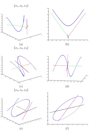
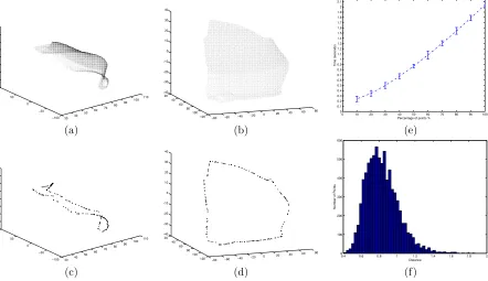
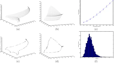
In order to see the meaning of the eigenvalues of G, let us consider the following example. A curve inR4_{is built from two 2}_D_{quadratic forms, which, in this particular}

case, are an ellipse and a hyperbola (see ﬁg. 6.2). This may be an example of generating a real spaceℜ4_{from the direct sum of lower dimensional subspaces. Now,}

we can see that the matrixGthat generated the orbit, with some initial condition, has two complex eigenvalues and two real ones. Indeed, under a similarity transformation T,Gcan be written as follows:

G=T    

0 ω 0 0

−ω 0 0 0

0 0 λ1 0

0 0 0 λ2

   T

−₁

where_{iω,₋iω_} are pure imaginary eigenvalues of G, and _{λ1, λ2} are real values.

In this particular case, we take λ1 to be a real positive number, and λ2 to be a

negative real number. From this information, we can see that the _ℜ4 _{space is}

de-composed in 3 subspaces, Ec _{= [span}

{e1, e2};{iω,−iω}], Eu = [span{e3};λ1] and

Es_{= [span}_{_e

4};λ2]. Takingφ(0) = [x1(0), x2(0), x3(0), x4(0)] as inital condition, the

parametric equation of the orbit, i.e. the solution of eq. (6.2) in this particular case is:

φ(θ) = T eΛθT−1_φ_{(0) =}

= T    

cosωθ sinωθ 0 0

−sinωθ cosωθ 0 0

0 0 eλ1θ ₀

0 0 0 eλ2θ

   T

−1_φ₍₀₎

(16)

{x1, x2, x3}

−5 0 5 −1 0 1 2 3 4 5 −4 −3 −2 −1 0 1 2 3 4

−5 −4 −3 −2 −1 0 1 2 3 4 5 −0.5 0 0.5 1 1.5 2 2.5 3 3.5 4 4.5 (a) (b)

{x1, x4, x3}

−5 0 5 −4 −2 0 2 4 −4 −3 −2 −1 0 1 2 3 4 −5 −4 −3 −2 −1 0 1 2 3 4 5 −5 0 5 −4 −3 −2 −1 0 1 2 3 4 (c) (d)

{x4, x3, x2}

−4 −3 −2 −1 0 1 2 3 4 −1 0 1 2 3 4 5 −4 −3 −2 −1 0 1 2 3 4

[image:16.595.135.432.179.617.2]

−4 −3 −2 −1 0 1 2 3 4 −4 −3 −2 −1 0 1 2 3 4 (e) (f)

Figure 6.2: 3-Dimensional projections of a solution of a linear dynamical system in 4D. Plot (b) is another view of (a),where the meaning of two (generalized) eigenvectors is interpreted as the asymptotes of Eu_{. Plot (f) shows the axis that}

(17)

6.3. Appearance Based Framework for Time Symmetry Estimation 133

From this solution, we deduce that Ec _{= span}

{e1, e2} (purple and black axis

direc-tions in ﬁg. 6.2 (f)) is an invariant subspace that generates a closed orbit, Eu ₌

span_{e3} (red axis direction in ﬁg. 6.2(b))is an invariant subspace of solutions that

decay to zero asθ _{→ −∞}, andEs_{= span}

{e4} (green axis direction in ﬁg. 6.2(d))is

the third invariant subspace of solutions that decay to zero asθ→ ∞. For instance, consider an initial condition like the following:

T−1_φ_{(0) =}

   

x1(0)

x2(0)

0 0

   

Therefore, orbit obtained by means of (6.3) remains in Ec _{= span}_{_e

1, e2} for all

possible values of the time parameter θ, and that fact is in accordance with the deﬁnition 6.2.1.

With this reference to the analysis of the solutions of linear dynamical systems, we see that the information, which is encoded in the inﬁnitesimal generatorG, is straight forward understandable through its eigenvalues and eigenvectors. This internal struc-ture analysis not only allows the selection of a new representation for the images evolution, which is based in the modes ofG(eigenvectors), but also yields a manner of grouping the diﬀerent principal directions ofG distinguishing the subspaces that they span in terms of stability, i.e.,Eu,EsandEc.

6.3 Appearance Based Framework for Time

Sym-metry Estimation

The previous example was performed in order to illustrate that a sequence of points that follow a certain temporal evolution can be described in terms of some privileged directions which are indicative of the behavior of the curve where they are embedded into. The aim of this is to apply linear dynamical system theory to temporal corre-lated sequences of images. To this end, we need to deﬁne a feature space where the images can be represented as points. Subsequently, the goal is to have an estimation of the evolution process of these images. The aim of this is to extract the tempo-ral information encoded in the inﬁnitesimal generator in order to present a reduced number of images that are able of summarizing semantically the whole sequence.

In this section, we present a generative model which deﬁnes appearance represen-tation and time evolution between consecutive frames. This model involves jointly representation and evolution of appearance. In this case, temporal symmetry estima-tion is based on the fact that images belonging to a coherent sequence are also related by means of appearance representation.

(18)

6.3.1 Appearance Representation Model

First of all, we need to define a space of features where images are represented as points. This problem involves to find a representation as a support for analyzing the temporal evolution. To address the problem of appearance representation, authors in [106, 77, 68] proposed Principal Component Analysis as redundancy reduction technique in order to preserve the semantics, i.e. perceptual similarities, during the codification process of the principal features. The idea is to find a small number of causes that in combination are able to reconstruct the appearance representation. These small numbers of causes are taken as the basis for the feature space. Besides, Tipping et. al. [15] embedded PCA into a Linear Generative Model framework in order to capture the intrinsicdegrees of freedom of the object category model as well as to give an inherentlikelihood measure to the learned object category. Generative models are a causal approach to describe the underlying phenomena that generates the complexity of observed data (images).

One of the most common approaches for explaining a data set is to assume that causes in linear combination:

t=W x+µ+e

where x _{∈ ℜ}q _{(our chosen reduced representation,} _{q < d}_{) are the causes (latent}

variables), W is an orthogonal matrix which rotates the data t, µ corresponds to the sample mean and e is some noise. This causal approach leads to deﬁne a joint distributionp(t, x) over visible_{t_}and hidden variables_{x_}, the corresponding distri-butionp(t) (similarity measure) for the observed data is obtained by marginalization: p(t) = , p(t_|x)p(x)dx, where p(t _| x) deﬁnes the causal connection between the observations{t} and the latent variables{x}, and it is associated to the noise distri-bution as follows:

p(t|x) = 1 (2πσ2₎d/2exp

−₂1_σ₂ |t−µ−W x|2

and the corresponding similarity measure given the model:

p(t) = 1

(2π)d_det_Cexp

−1₂(t−µ)TΣ−1₍_t

−µ)

where Σ = W WT ₊_σ2_I_{. The} _prior _{knowledge on latent variables is expressed}

in p(x). This density function takes the form of a Gaussian distribution with zero mean and identity covariance matrix: _N(0, I). Therefore, it is said that the causes are mutually independent in terms of a second order statistics. The main goal is to find the parameters that maximize the joint observed data distribution i.e. the best description under the specific generative model. After considering the temporal model, the algorithm to estimate latent variables and parameters is introduced in a unified framework for appearance representation and evolution.

6.3.2 Appearance Temporal Evolution Model

(19)

6.3. Appearance Based Framework for Time Symmetry Estimation 135

S. On the other hand, equation (6.1) can be interpreted in terms of a generative model, where an image description in latent spacexn+1 is obtained making to evolve

with the actionG, and a certain quantity θn, a previous onexn.

Symmetry learning is based on observations, more speciﬁcally, in a sequence of ordered images. So, is feasible to consider that observations are obtained with a certain additive noise. The generative equation takes the following form:

x(θ) =eθG_x_{(0) +}_r _(6.4)

whereris aθ-independent noise process. According to the inﬁnitessimal approxima-tioneθG

∼1 +θG, eq. (6.4) yields:

x(θ) = (1 +θG)x(0) +r

∆x(θ) = θGx(0) +r (6.5)

where ∆x(θ)≡x(θ)−x(0). For the isotropic noise model caser∼ N(0, β2_I_{), the}

probability distribution over the transformations ∆x-space for a given image x_{∈ S} and step parameterθ corresponds to:

P(∆x|x, θ, G, β2) =

= 1

(2πβ2₎q/2exp

−₂_β12 |∆x−θGx| 2

The prior distribution over the latent variables θ is assumed to be Gaussian with unit variance, so θ _{∼ N}(0, I). Therefore, the corresponding similarity measure for temporal transformations in latent space S is obtained by marginalization:

P(∆x|x, G, β2) =

P(∆x|x, θ, G, β2)P(θ)dθ=

= 1

(2π)d√_det_Cexp

−1₂∆xTC−1_∆_x

(6.6)

whereC=GxxT_GT₊_β2_I_{. The similarity measure eq. (6.6) evaluates the likelihood}

of a transformation ∆xbetween to points,(for a given xn to a following onexn+1),

respect to a learned model _{G, β2

}. These points _{xn, xn+1} are a representation

of two images _{tn, tn+1} for a certain instance of the appearance model {W, µ, σ2}.

Indeed, this probabilistic framework allows determining whether two consecutive im-ages are in accordance with the learned dynamical model. This fact has an important signiﬁcance when it comes to assign some boundaries to a sequence of frames.

6.3.3 Maximum Likelihood Estimation

At this point, the problem is centered on parameter estimation, which, in practice, will be given by data observations. This leads to consider the problem ofincomplete data. For this purpose, Dempster et al.(1977) [31] use the EM algorithm, where each observation tn (image) is associated to an unobserved statesn={xn, θn}, and

(20)

given set of observations_{t1, . . . , tN} the likelihood measure to be maximized is the

Complete-log-Likelihood, i.e.:

L(y1, . . . , yN|Ω) = log{p(t1, . . . , tN;s1, . . . , sN |Ω)} (6.7)

where Ω represents the model parameters.

Although both parameters and latent variables are unobserved, the diﬀerence is that latent variables are pressumed to be instantiated once for every observation, that is there is a latent sn for each observation tn. Furthermore, the noise model oﬀers

smoothness, then, this approach diﬀers from regression-based methods, in the way that the goal is to estimate the data density, and leading to reduce the overﬁtting. The following table shows the paramaters Ω that are involved in the model, and the latent variables related tosn:

Model Generative Mapping Parameters,Ω sn

App,Rep. tn=W xn+µ+en W, σ2, µ xn

Time Sym, ∆xn=θnGxn+rn G, β2 _θn

Following the assumption that appearance representation depends only on data observations, the ML estimation for the appearance parameters is given in a closed form solution as it is developed in [15]:

W =Uq(Λq−σ2I)

1

2R; σ2= 1 d₋q

d

j=q+1

λj

whereUq are the ﬁrstqeigenvectors of the data set covariance matrix, Λqis a diagonal

matrix with the corresponding ﬁrst q eigenvalues (λi, ∀1 ≤ i ≤ N) and R is an

arbitrary rotation matrix.

In order to estimate the appearance dynamics we utilize an EM algorithm, which is detailed in the Appendix A. This is basically a two steps procedure: Expectation

and Maximization of a likelihood function. The Expectation step requires a third

operation, which in the latent variable model can be added to the pair of learning and model selection; inference. This refers to estimation of value of latent variables sn given known parameters Ω and observationstn.

The introduced model shows a hierarchical structure between observed images tn and latent variables xn, θn. First, images are obtained to build the appearance

representation, and secondly, taking avantage of a reduced appearance basis, data evolution is estimated. Inference is this framework is a simple matter of the applica-tion of Bayes’ rule:

1. Inferring latent variables related to apperance:

p(x_|t,Ω) = p(x)p(t|x,Ω)

(21)

6.4. Experimental Results 137

2. Inferring latent variables related to temporal evolution, given appearance latent variables inferred and their corresponding transformations computed:

p(θ_|x,∆x,Ω) = p(θ)p(∆x|θ, x,Ω)

p(∆x|x,Ω) (6.9)

Therefore, for each image tn the computation of its corresponding coordinates in

latent spacexn is given by means of the Maximum a Posteriori (MAP) in eq.(6.8):

x= argmaxx′p(x

′

|t,Ω) (6.10)

Once, images are expressed in latent space coordinates, the computation of the best estimated transformation parameterθn is also done through the MAP in eq.(6.9):

θ= argmaxθ′p(θ

′

|x,∆x,Ω) (6.11)

Under gaussian assumptions for noise models and prior knowledges, theposterior the posterior means< x|t > and< θ|x,∆x > correspond to the MAP for each distri-bution. In the appendix we show the explicit forms for these posterior probabilities, as well as, an EM algorithm for the temporal parameters estimation is introduced.

6.4 Experimental Results

In this section, we exemplify the application of the introduced appearance evolution model to the extraction of semantically meaningful image-like data structures. Two types of experiments are developed in this section. First, a study of the invariance subspaces derived from the estimation of the action G of the group is performed for periodic motions. Second, an application to summarization of video sequences is presented.

6.4.1 Capturing Local Behaviors through Global

Representa-tions

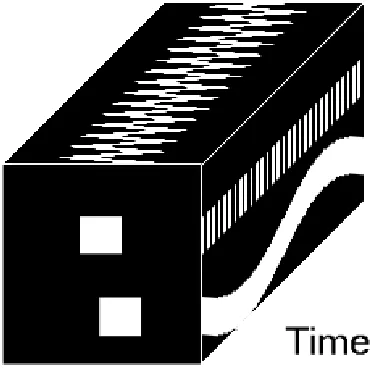
This first experiment has the purpose of studying the subspaces obtained from the eigenvector decomposition of the infinitesimal generator G. To this end, a synthetic sequences of images has been constructed. Figure 6.3 shows the temporal volume of this sequence of images. Two types of different periodic motions are present in the sequence. Their corresponding frequencies are significantly different.

Global Representation. The synthetic sequence consists of 100 images. Two white

(22)

[image:22.595.190.375.168.355.2]

Figure 6.3: Temporal volume representation of the synthetic image sequence with two oscillatory motions.

between the two types of motions is performed (see ﬁgure 6.4 (f)). They are designed to rank variations in the set of images from low to higher frequencies. In fact, no temporal correlation is taken into account when constructing a PCA representation.

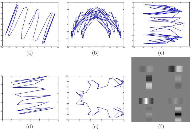
The PCA representation has been build using 4 Principal Components, that cope with the 70% of the total energy. Of course, more than 4 PC could have been selected. However, according to the previous analysis of the invariant subspaces, the aim is to divide the invariant orbits into two groups. Figure 6.4 shows the projected orbits onto pairs of Principal components. All of them, show that there is an inherent periodicity in the evolution of the trajectories.

Invariant Subspaces. Adding temporal correlation to this analysis, we can see that

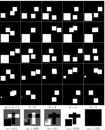
two subspaces can describe the two different motions. This study has been per-formed by running the presented EM algorithm for estimating the infinitesimal generatorGof the temporal evolution, the corresponding one-dimensional pa-rameter for each image. The eigenvector decomposition of the matrixGgives two invariant subspaces. The corresponding orbits are plotted in figure 6.5. More specifically, figure 6.5 (b) shows many repetitions of the same trajectory, while figure 6.5 (c) shows only one trace. This is not surprising since if we look at the temporal volume in figure 6.3, we can notice that there is one horizontal motion with a higher frequency than the vertical one, which just presents one oscillation.

(23)

−20 −15 −10 −5 0 5 10 15 20 −20 −15 −10 −5 0 5 10 15 20

−20 −15 −10 −5 0 5 10 15 20 −15 −10 −5 0 5 10 15

−15 −10 −5 0 5 10 15 −20 −15 −10 −5 0 5 10 15 20

(a) (b) (c)

−15 −10 −5 0 5 10 15 −15 −10 −5 0 5 10

−15 −10 −5 0 5 10 −20 −15 −10 −5 0 5 10 15 20

(d) (e) (f)

Figure 6.4: Plot (a) shows a projection onto the two ﬁrst appearance eigenvectors, (b) ontox2, x3,(c) ontox3, x1,(d) ontox3, x4,and (e) ontox4, x1. Figure (f) shows

the 4 eigenvectors obtained from PC Analysis.

−8 −6 −4 −2 0 2 4 6 8 −15 −10 −5 0 5 10

−8 −6 −4 −2 0 2 4 6 −4 −2 0 2 4 6 8 10

[image:23.595.135.499.165.411.2]

(a) (b) (c)

(24)

0 10 20 30 40 50 60 70 80 90 100 −0.04

−0.03 −0.02 −0.01 0 0.01 0.02 0.03 0.04

0 10 20 30 40 50 60 70 80 90 100 0

0.2 0.4 0.6 0.8 1 1.2 1.4

(a) (b)

Figure 6.6: Representation of the temporal evolution of the one dimensional pa-rameter θ in (a),and its Fourier Transform power spectrum in (b). Clearly,two frequencies are signiﬁcantly noticeable.

of the the two sets of eigenvectors inG, leads to a meaningful description of the local behaviors of the two different motions in the frame of reference. In fact, they can be seen as masks that locally segment the regions where one of the two motions occurs. The image pair in the top of figure 6.5 (a) shows a segmentation of the area where the faster horizontal motion happens. Analogously, the area in the two images of the bottom of figure 6.5 (a) describe the slower vertical motion.

This local segmentation has been performed through a suitable global represen-tation that takes into account both temporal evolution and invariance at the same time.

ExtractingInformation from θ. The estimation of the one-dimensional

param-eter of the evolution for image also gives a notion of the two periodicities. Transforming the temporal evolution ofθ(t) into the Fourier power spectrum representation, we can notice that two main frequencies are remarked. The ac-curacy when determining frequencies by means of this method, or through the imaginary parts of the eigenvalue analysis of the matrixG depends on the re-construction error of the selected appearance representation. Nevertheless, this technique can be used as an estimator of potential periodic motions in video se-quences. This fact makes feasible an enrichment on automatic video annotation systems. Chapter 8 shows another technique to discriminate periodic motions based on a local representation of the pixel values variations.

6.4.2 Key-Frames Extraction

(25)

(a)

(b)

(c) (d)

[image:25.595.200.428.145.709.2]

(e) (f)

(26)

(a) (b)

(c)

(d) (e)

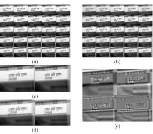
Figure 6.8: (a) Original sequence of frames. Reconstructed sequence (b) with 88.17% of reconstruction quality using 4 principal components of appearance (e) and a 4×4Gmatrix whose eigenvectors correspond to the images (c) and (d).

0 1 23 45 67 8 9 10 11 12 13 14 15 16 17 18 19 20 21 22 23 24 25 −1

−0.8 −0.6 −0.4 −0.2 0 0.2 0.4

Points Index

Time Step

0 1 2 3 4 5 6 7 8 9 10 11 12 13 14 15 16 17 18 19 20 21 22 23 24 25 26 27 28 29 30 −0.7

−0.6 −0.5 −0.4 −0.3 −0.2 −0.1 0

Points Index

Time Step

[image:26.595.129.437.166.437.2]

(a) (b)

(27)

necessary to build the appearance representation by means of the ML for PPCA. Afterwards, utilizing the posterior probability eq. 6.8, the new coordinates for the images are computed though MAP. We use these new appearance representation to estimate the dynamical model by means of the introduced EM algorithm (see appendix). Once G is estimated we compute the iconic representation, by means of an eigenvector analysis the inﬁnitesimal generator. These eigenvectors are back-projected to the image space in order to have an expression of them as images.

The first sequence, fig. 6.7 (a), is represented by a 2-dimensional appearance eigenspace with a 70.45% of reconstruction quality. The appearance eigenvectors rep-resented as images are shown in fig. 6.7(e) and (f). These express the variations between the mean or prototypical appearance of the object. However, such a proto-type is not an appropriate representative sample, since the concept of ”face” is not as much perceptible as in figs. 6.7(c),(d). Performing the estimation of the dynamical model{G, β2_}_{, we have the corresponding generator of the transformation os a 2}_×₂

matrix whose modes correspond to the images fig.6.7 (c),(d). They are presented like real images, however, they are not directly obtained from the sequence, i.e., like selecting the first frame and last one. The significant issue here is that this temporal information can be used to reconstruct the video sequence (fig. 6.7 (b)) by means of eq. (6.5) and using just only the 2_×2 matrix, the appearance basis and the time step θn of the evolution, (see fig. 6.9(a)).

The purpose of this second one sequence (fig. 6.8) is to expose that the appearance evolution model does afford to keep perceptually the camera operation in the new iconic representation. Given that editors, authors and artist communicates some specific intentions with certain camera operations, we notice that this information remains in the summarized representation. This sequence of frames (fig. 6.8(a)) has been represented in a 4-dimensional subspace with a 88.17 % quality of reconstruction. The 4 eigenvectors of appearance fig. 6.8(e) do not give a semantically meaningful idea of the images evolution, actually, we can see that they point out some zones of the image where the variations, at different scales, are produced. The temporal evolution was estimated by a 4_×4 matrix, whose principal directions are represented as images in fig. 6.8 (c) and (d). They correspond to 2 complex (and conjugates) eigenvalues ofG. So, using the theoretical background in LDS, we deduce that they are grouped in two classes, forming 2 invariant spaces: two vectors in fig. 6.8(c) and the other two in fig. 6.8(d). We can see what each one of them is expressing by focussing in the sign’s letters of the images. The two first ones, fig. 6.8(c), are centered on a slow frequency (in time) variation, the sign is clearly readable and some blur only appears in the images’ boundaries. The 2 second ones fig. 6.8 (b) are more focussed in high frequency time variations. We notice that the word ”SOM” appears at separate different distances. The termfrequency is applied here to the imaginary part of the complex eigenvalues. Actually, the frequency of the eigenvectors in fig. 6.8(c) isω1= 0.36, and the frequency of the eigenvectors in fig. 6.8 (d) isω2= 0.61.

Therefore, we note that there is a direct relation between the imaginary values of G-eigenvalues and movement variations in the iconic representations.

(28)

of reconstructing the sequence with a small number of parameters: figs. 6.7 (b) and 6.8(b). This fact allows the possibility of performing video preview with a low cost of streaming, and it is very appropriate for low bandwidth communication systems (like a modem at home). To this end, we need the eigenvectors that span the appearance representation, the matrix G (2×2 in fig. 6.7 and 4×4 in fig. 6.8), the reduced coordinate of the first image, and an 1-Darray of scalar values that represents the time step evolution from image to images. Thus, utilizing eq. (6.5) as a filtering process, the whole sequence is reconstructed. Note that our model includes an estimation of the time step between consecutive images (see figs. 6.9 (a),(b)), what differs from dynamical models that assume a constant time step evolution.

6.5 Summary and Conclusions

As an alternative to standard key-frames selection, in this chapter we propose a Bayesian framework for video summarization. We address the problem of character-izing key-frames basing partitions on appearance visual information criterion and, at the same time, conjugating semantic and temporal representations. This fact, not only allows embedding in a more numerical tractable framework the videoretrieval, but also yields a new approach to extract underlying information from temporal evo-lution of sequences. A suitable selection of these basic perceptual units allows the transformation of a continuous temporal data structure into a discrete meaningful one, where the intention is that the semantics remains preserved. The choice of an appropriate representation for the data takes a signiﬁcant relevance when it comes to deal with symmetries, since these usually imply that the number of intrinsic degrees of freedom in the data distribution is lower than the coordinates used to represent it. Indeed, this means that the problem can be reduced to a lower dimensional one. Therefore, using both topics; the decomposition into basic units and the change of representation, makes that a complex problem is transformed into a manageable one. This simpliﬁcation of the estimation problem has to rely on a proper mechanism of combination of those primitives (appearance eigenvectors) in order to give an optimal description of the global complex model.

Appendix: EM algorithm for Maximum Likelihood

Estimation

In the Expectation-Maximization (EM) algorithm for symmetry estimation, we con-sider the latent variables θn to be ”missing”. If their value were known, the

(29)

6.5. Summary and Conclusions 145

model. Assuming that we do not know for a given transformation ∆xn which value

ofθn generated it, the joint distribution can be calculated through theexpectation of

thecomplete data log-likelihood.

From a Bayesian point of view, Maximum Likelihood estimation requires, in gen-eral, a two step procedure:

1. Expectationof latent variablesθnfor a given observed ∆x. Posterior expectation

given observed data for the complete log-likelihood is a way of computing an aproximation of the predictive density.

2. Maximisationof complete log-likelihood from the model parametersG, σ2_{. This}

is equivalent to minimize the expectation of the loss function under that (ap-proximated) predictive density.

Expectation The expected complete-data log likelihood is given by:

<L> =

N−1

n=0

1

2σ2 <|∆xn−θnGxn| 2_>₊

+ q 2logσ

2₊< θ2n>

2

which expanded yields:

L =

N−1

n=0

1

2σ2 |∆xn| 2₊ 1

2σ2 < θ 2

n> xTnGTGxn−

− ₂_σ1₂ < θn> xTnGT∆xn− − ₂_σ12 < θn>∆x

T nGxn+

< θ2

n>

2

+N q 2 logσ

2

where the suﬃcient statistics of the posterior distributions correspond to:

< θn> = M−1_xT

nGT∆xn (6.12)

< θ2n> = σ2M

−₁

+< θn>< θn> (6.13) withM =σ2₊_xT

nGTGxn.

Maximization Diﬀerentiating equation (6.12) and setting the derivatives to zero,

Gandσ2 _{are updated as:}

ˆ

G =

n

< θn>∆xnxTn

n

< θn2 > xnxTn −₁

σ2 = 1

N q N

n=1

|∆xn|2−2< θn> xTnGˆT∆xn+

(30)

(31)

Chapter 7 Online Bayesian Video

Summarization and Linking

In this chapter,an online Bayesian formulation is presented to detect and describe the most significant key-frames and shot boundaries of a video sequence. Visual information is encoded in terms of a reduced number of degrees of freedom in or-der to provide robustness to noise,gradual transitions,flashes,camera motion and illumination changes. We present an online algorithm where images are classified according to their appearance contents -pixel values plus shape information- in order to obtain a structured representation from sequential information. This structured representation is presented on a grid where nodes correspond to the location of the representative image for each cluster. Since the estimation process takes simulta-neously into account clustering and nodes’ locations in the representation space, key-frames are placed considering visual similarities among neighbors. This fact not only provides a powerful tool for video navigation but also offers an organization for posterior higher-level analysis such as identifying pieces of news,interviews,etc.

7.1 Introduction

R

ich Media and content management has generated an enormous interest in video analysis within Computer Vision and Pattern Recognition communi-ties. It offers a novel and exciting challenge for applying and developing new techniques in the recognition/classification framework. The addition of time to visual information analysis presents new constraints -a huge amount of information to be dealt with- and specific demands (such as real-time analysis) on the formulation of feasible and reliable techniques.

In this chapter, we focus on two important subjects in this area: video segmenta-tion and summarizasegmenta-tion, which make feasible a quick intuisegmenta-tion of the evolusegmenta-tion, under

(32)

148 ONLINE BAYESIAN VIDEO SUMMARIZATION AND LINKING

a low streaming cost, of higher-level perceptual structures, such as stories, scenes or pieces of news. Shot partitioning is considered as the extraction of the basic units for video analysis. Usually, shot boundary detection has been analyzed through feature based techniques, such as: pairwise pixel comparison [117], which are very sensitive to noise, color or grayscale histogram comparison [95, 115], which fails in distinguish-ing images with very different structures but similar color distributions, analysis of compressed streams [2, 3], and local feature based techniques [116]. However, many problems arise when it comes to dealing with noise, shape information, camera mo-tion, illumination change, fades, and flashes. In these cases, specific problem-oriented techniques are applied: camera compensation [117], illumination reduction [119]. This sort of peculiarities are also treated by combining different measures [27]: dissolve, cut and fade measures. On the other hand, appearance based methods [38] use a representation where visual changes are encoded with a reduced number of degrees of freedom, and which provide more flexibility to the system in order to tolerate camera motions or illumination changes. However, the method presented in [38] requires load-ing the whole sequence. Offline techniques are not practical when dealload-ing with large pieces of video. In this sense, online solutions, combined with certain robustness to gradual transitions and a reasonable computational complexity, are rather preferable.

To this end, we present a novel algorithm that provides an online treatment of video analysis plus the mentioned advantages of working under a Bayesian appearance-based framework. We address the problems of key-frame extraction and shot parti-tioning relying on a feature space where not only pixel value distributions (grayscale or color) are encoded but also shape information is taken into account. The algorithm online classifies the different shots of a video sequence and automatically extracts the most significant key-frames. Often, due to postproduction work (in commercials, movies, etc.), there are many sequences that contain the same shot in different time positions, that make standard algorithms to produce repeated key-frames and forcing posterior ad hoc merging/removing techniques in order to avoid unnecessary redun-dancies. Given that the algorithm is embedded in a Bayesian formulation, questions such as sufficient number of key-frames to represent a video sequences or avoiding extra key-frame detection due to flashes, are automatically solved.

The problems of key-frame extraction and shot partitioning are treated in terms of a probabilistic unsupervised learning approach. Each frame of a video sequence is assumed to belong to a cluster of images that are related in terms of their appearance contents, and, each cluster has a representative image that will be used for summa-rization purposes, i.e., a key-frame. The algorithm’s process is controlled by a tuning parameter whose range embraces appearance representation [97, 67, 106] (such as PCA, FA or NNMF techniques) and hard clustering (competitive learning). The goal of the learning is to identify the latent variables (weights) and the unknown mapping parameters (key-frames). For this purpose, we present the estimation process in the context of the Expectation-Maximization algorithm.

(33)

7.2. The Model: Bayesian Framework 149

parameters of the model in two versions: offline and online. The experimental results analyze: (i) the effects of the tuning parameter that makes the algorithm embracing techniques compressed representation of appearance and clustering techniques, (ii) the effectiveness of dealing with prior information in order to automatically select the number of necessary key-frames to represent a video sequence.

7.2 The Model: Bayesian Framework

In order to describe our model, we ﬁrst deﬁne the latent space were observations (images) are represented. We consider this latent space to be a grid of M nodes represented by a set of vectors{c1, . . . ,cM}. Each node represents a class of images

that are similar in terms of their appearance contents. Consider a set of N images {y1, . . . ,yN} in a vector form read in lexicographic order, and each image

represen-tation (location) on the 2D grid (latent variables) as{x1, . . . ,xN}. For each latent

variablexnwe like to know the contribution to its generation for each nodecmin the

grid. A measure that quantiﬁes such a contribution can be expressed in terms of a Bayesian framework by the posterior probabilityP(cm|xn). The model will provide

the similarity measure that relates the ownership of an image under a speciﬁc class. Consider each nodecm has a representative imagewmthat summarizes the images’

appearance contents that belong to them-class. In this sense, we can consider each image to be a weighed combination of the summarizing representative images wm,

where the weights correspond to the posterior probabilitiesP(cm|xn).Therefore, we

can construct a model where images and latent variables (2D points on the grid) are related by the following mapping:

yn=

M

m=1

wmP(cm|xn) +en (7.1)

where en is gaussian independent identically distributed (idd) noiseN(0, σ2I).

Al-though equation (7.1) has the form of well known linear decompositions, PCA or FA, it is worth noting that the posterior probabilities P(cm | xn). are restricted to be

non-negative and the sum to be the unity. In the following sections, we show that the nature of these posterior probabilities determines whether the model can be used for performing hard clustering (key-frame extraction and shot partitioning applications) or a compressed representation of images (dimensionality reduction). The model has two main issues: on one hand, the estimation of the representative images wm and

the posterior probabilitiesP(cm|xn), and on the other, the inference for the images’

location in the latent space (grid).

Noise model

First, the noise model is expressed through a Gaussian distribution for the data: N(yn−Whn, σ2), where W is a matrix whose columns are the vectorswmandhnis an

(34)

150 ONLINE BAYESIAN VIDEO SUMMARIZATION AND LINKING

A Bayesian treatment of this model is obtained by introducing a prior distribution over the components _{w1, . . . ,wM}. The key point is to control the eﬀective

num-ber of suﬃcient parameters (numnum-ber of classes). This is achieved by introducing a prior distributionP(W |α), whereαis a M-dimensional vector of hyper-parameters {α1, . . . , αM}. Each hyper-parameter αm controls one of the cluster representative

vector wm by means of the following distribution: P(W | α) = M_m₌₁N(wm, α−m1)

Each hyper-parameter αm corresponds to an inverse variance. For large values ofα

the corresponding wm will tend to be small, and therefore, such component will be

neglected. These hyper-parameters behave as switchers, activating or deactivating each component wm. Typically, the selection for the distribution of αm corresponds

to Laplace distributions or Gamma distributions due to their properties on ”pruning”. We select a gamma distribution for the hyper-parameters, since it oﬀers a tractable analytical treatment for the estimation process: P(α) =M_m₌₁Γ(αm|a, b), where

Γ(αm|a, b) =

ba₍_α

m)a−1e−bαm

Γ(a) (7.2)

We selecta= 10−3_and _b_{= 10}−3_{, which are the magnitude orders typically selected}

in this framework.

Modelingthe latent space

The distribution on the grid is modeled as a mixture of unimodal distributions. For instance, one might select a mixture of Gaussians, however, the algorithm that we present can be easily modiﬁed with another type of density functions (laplacians, gamma, etc.). The likelihood measure for a single point in the latent space is given by: P(xn) =M_m₌₁P(cm)P(xn |cm), where we select the conditional distributions

to have the form of Gaussian distributions: P(xn|cm) =N(xn−cm, τm2).

7.2.1 Parameter Estimation

In this section, we present the framework where the parameters of this model are estimated. The estimation process has to take into account two issues at the same time: the noise model and the density distribution in the latent space. In the estima-tion procedure, there are two main steps communicated by a feedback process. Given a set of images, the cluster representative images wm and the posterior probability

vectors are computed in order to infer the location of each image on the grid. This is done through posterior expectation of the nodes, i.e.:

< xn >= M

m=1

cmP(cm |x_n) =

M

m=1

cmhmn (7.3)

These expected locations on the grid are used as data for estimating the grid’s den-sity distribution parameters, i.e., the variancesτ2

m, which play an important role as

(35)

7.2. The Model: Bayesian Framework 151

probabilities are then recomputed using the Bayes’ rule. Since these probabilities con-tribute to the re-estimation of the componentswm, now, the estimation of the noise

model parameters takes into account the topographical distribution of the clusters in the latent space.The following table summarizes the parameters to be estimated according to these two steps:

Model Parameters Noise wm hn σ2 αm

Cluster representative images Posterior Probabilities Noise variance Switchers Latent Space <xn>

τm

Expected location Node variance

We embed the estimation process in the framework of the Expectation-Maximization (EM) algorithm, which is useful to ﬁnd maximum likelihood parameter estimates in problems where some variables are unobserved. In our case, posterior probabilities and posterior location points are unobserved. The M step maximizes w.r.t. the model parameters (wm, σ2, αm, τm) and the E step maximizes it w.r.t. the distribution over

the unobserved variables (hn, <xn >). Typically, the algorithm consists of a set of

ﬁxed-point type equations that are iterated until convergence. In the following sec-tion, we show the procedure to estimate both sets of parameters and latent variables.

EM Algorithm

The maximum likelihood estimation for the noise model parameters can be equiva-lently performed in terms of maximizing the logarithm of the joint distribution:

L=−1₂ N

n=1

|yn−Whn|2 −

1 2 M m=1

αm|wm|2+ d

2logαm−log Γ(αm|a, b)

(7.4) Given an initial guess for the parameters and unobserved variables iterate:

• Expectation: Find hn that maximizes (7.4). Given the constraints for hn

-non-negativity and normalization- we need to apply a exponentiated gradient method [55] to ensure that the new estimates are always positive. This is done by introducing an auxiliary function as in [31]. In order to derive this update rule, we make use of an auxiliary functionG(hn,htn) such thatG(hn,hn) =L(hn)

and G(hn,htn)≤ L(hn) for allhtn. For this auxiliary function, it can be seen

that F is nondecreasing after the updateht+1

n = arg maxhnG(hn,h

t

n). So the

update rule is given by making∂G(hn,htn)/∂hn = 0 on each step. An auxiliary

function for L(hn) is constructed as,

G(hn,htn+1) =−

1 2

N

n=1

|yn−Whtn+1|2−ν M