ADVERTIMENT. La consulta d’aquesta tesi queda condicionada a l’acceptació de les següents condicions d'ús: La difusió d’aquesta tesi per mitjà del servei TDX (www.tesisenxarxa.net) ha estat autoritzada pels titulars dels drets de propietat intel·lectual únicament per a usos privats emmarcats en activitats d’investigació i docència. No s’autoritza la seva reproducció amb finalitats de lucre ni la seva difusió i posada a disposició des d’un lloc aliè al servei TDX. No s’autoritza la presentació del seu contingut en una finestra o marc aliè a TDX (framing). Aquesta reserva de drets afecta tant al resum de presentació de la tesi com als seus continguts. En la utilització o cita de parts de la tesi és obligat indicar el nom de la persona autora.
ADVERTENCIA. La consulta de esta tesis queda condicionada a la aceptación de las siguientes condiciones de uso: La difusión de esta tesis por medio del servicio TDR (www.tesisenred.net) ha sido autorizada por los titulares de los derechos de propiedad intelectual únicamente para usos privados enmarcados en actividades de investigación y docencia. No se autoriza su reproducción con finalidades de lucro ni su difusión y puesta a disposición desde un sitio ajeno al servicio TDR. No se autoriza la presentación de su contenido en una ventana o marco ajeno a TDR (framing). Esta reserva de derechos afecta tanto al resumen de presentación de la tesis como a sus contenidos. En la utilización o cita de partes de la tesis es obligado indicar el nombre de la persona autora.
Arithmetic Properties of non-hyperelliptic
genus 3 curves.
Elisa Lorenzo García
Universitat Politècnica de Catalunya
Advisor: Joan-Carles Lario Loyo
Contents
Introduction 3
Preliminars 7
1 Twists of non-hyperelliptic curves 11
1.1 Galois embedding problems . . . 11
1.2 Equations of the twists . . . 12
1.3 Description of the method . . . 13
1.4 An example . . . 16
2 Non-hyperelliptic genus 3 curves 21 2.1 Henn classification . . . 22
2.2 Modified Henn classification . . . 23
2.3 A representative in the modified Henn classification . . . 29
3 Twists of non-hyperelliptic genus 3 curves 35 3.1 The Fermat quartic . . . 35
3.2 Cases from I to X . . . 45
3.3 The Klein quartic . . . 51
4 The Sato-Tate conjecture for the twists of the Fermat and Klein quartics 61 4.1 The Sato-Tate conjecture . . . 62
4.2 The Sato-Tate groups . . . 62
4.3 The Sato-Tate distributions . . . 66
4.4 Example curves . . . 67
5 The Sato-Tate conjecture for the Fermat hypersurfaces 69 5.1 Etale cohomology´ . . . 69
5.2 Jacobi sums . . . 71
5.3 Sato-Tate groups . . . 77
5.4 Proof of the conjecture . . . 79
5.5 An example . . . 79
Appendix 85
Inverse Galois problems . . . 85 Tables . . . 90
Abstract
We develope an algorithm for computing the twists of a given curve assuming that its auto-morphism group is known. And in the particular case in which the curve is non-hyperelliptic we show how to compute equations of the twists. The algorithm is based on a correspon-dence that we establish beetwen the set of twists and the set of solutions of a certain Galois embedding problem. As an application to our algorithm we give a classification with equa-tions of the twists of all plane quartic curves, that is, the non-hyperelliptic genus 3 curves, defined over any number field k.
The study of the set of twists of a curve has been proven to be really useful for a bet-ter understanding of the behaviour of the Generalize Sato-Tate conjecture. We prove the Sato-Tate conjecture for the twists of the Fermat and Klein quartics and we compute the Sato-Tate groups and Sato-Tate distributions of them.
Following with the study of the Generalize Sato-Tate conjecture, we show how to compute the Sato-Tate groups and the Sato-Tate distributions of the Fermat hypersurfaces: Xm
n ∶ xm
0 +...+xmn+1 =0. We prove the Sato-Tate conjecture for them when they are considerd to
be defined over Q(ζm).
Introduction
This thesis explores the explicit computation of twists of curves. We develope an algorithm for computing the twists of a given curve assuming that its automorphism group is known. And in the particular case in which the curve is non-hyperelliptic we show how to com-pute equations of the twists. The algorithm is based on a correspondence that we establish beetwen the set of twists and the set of solutions of a certain Galois embedding problem. In general is not known how to compute all the solution to a Galois embedding problem. Through the thesis we give some ideas of how to solve these problems.
The twists of curves of genus≤2 are well-known. While the genus 0 and 1 cases go back from long ago, see [55], the genus 2 case is due to the work of Cardona and Quer [8], [9]. All the genus 0, 1 or 2 curves are hyperelliptic, however for genus greater than 2 almost all the curves are non-hyperelliptic.
As an application to our algorithm we give a classification with equations of the twists of all plane quartic curves, that is, the non-hyperelliptic genus 3 curves, defined over any number field k. The first step for computing such twists is providing a classification of the plane quartic curves defined over a concrete number field k. The starting point for doing this is Henn classification of plane quartic curves with non-trivial automorphism group over
C.
An example of the importance of the study of the set of twists of a curve is that it has been proven to be really useful for a better understanding of the behaviour of the Generalize Sato-Tate conjecture, [16], [18], [21], [22]. We show a proof of the Sato-Tate conjecture for the twists of the Fermat and Klein quartics as a corollary of a deep result of Johansson, [34], and we compute the Sato-Tate groups and Sato-Tate distributions of them.
Following with the study of the Generalize Sato-Tate conjecture, in the last chapter of this thesis we explore such conjecture for the Fermat hypersurfaces Xm
n ∶ xm0 +...+xmn+1=0.
We explicitly show how to compute the Sato-Tate groups and the Sato-Tate distributions of these Fermat hypersurfaces. We also prove the conjecture over Q for n=1 and over Q(ζm)
if n≠1.
Content of chapters
In the first chapter of this thesis we describe an algorithm for computing the twists of curves via a correspondence between the twists and certain solutions to a Galois embedding prob-lem, section (1.1). In section (1.2) we show how to compute equations for the twists when the curve is non-hyperelliptic. We give a detailed descripcion of the algorithm in section (1.3). Finally, for illustrating the algorithm, in section (1.4), we show a complete example of the computation to the twists and its equations of a genus 10 non-hyperelliptic curve.
In chapter 2 we do the preparations for giving a classification of the twists of all non-hyperelliptic genus 3 curves defined over a given number field k. In section (2.1) we show a classification due to Henn of the plane quartic curves with non trivial automorphism group, up to C−isomorphism. In section (2.2) we modify this classification for getting it up to k−isomorphism. Finally, in section (2.3) we show, given any plane quartic with nontrivial automorphism group, how to find its representant in such classification.
After the results in chapter 2 we are ready for computing the twists of all plane quartic curves. In chapter 3 we give the classification of all such twists. In section (3.1) (resp. section 3.3) we compute the twists of the Fermat (resp. Klein) quartics, that are the harder cases, in part due to the fact that are, up to isomorphism, the two plane quartic curves with a biggest automorphism group. In section (3.2) we compute the twists of the rest of plane quartic curves. Just mentioning that this classification of the twists of the plane quartic curves is not totally complete, because we have not been able of computing a single case for the Klein quartic. The problem is that we have not been able of completely solving the corresponding galois embedding problem, so there is a single family of solutions/twists that we could not compute explicitly.
In chapter 4 we apply the former computations for computing new Sato-Tate distribution among the twists of the Fermat and Klein quartics. In section (4.1) we show a proof of the generalize Sato-Tate conjecture for these twists. The corresponding Sato-Tate groups and Sato-Tate distributions are computed in sections (4.2) and (4.3) respectively. Finally, in section (4.4) we show concrete examples of curves that attains such differente distributions and that have the corresponding Sato-Tate groups computed.
In chapter 5 we follow with the study of the Generalize Sato-Tate conejcture, but this time, we focus our study on the Fermat hypersurfaces Xm
n ∶ xm0 +...+xmn+1 =0. In (5.1) we
INTRODUCTION 5
the Jacobi Sums, both things will be necesary for computing the Sato-Tate groups in (5.3). In (5.4) we prove the conjecture over Q for n =1 and over Q(ζm) if n≠1. Finally we show
a complete example in (5.5).
In the first part of the appendix we establish a correspondence between the solutions to a given Galois inverse problem and rational points in a certain variety that we explicitly show how to compute via an algorithm. This can useful for trying to solve Galois embedding problems as the ones that appear in section (1.1) for computing the twists of curves. Our idea is, once the algorithm will be implemented, try to find the missed solution of the Galois embedding problem corresponding to the Klein quartic.
Finally, in the last part of the appendix we show tables with all the data computed through out the thesis: automorphism groups of the families of plane quartic curves in Henn classification and in the modified one, Dixmier-Ohno invariants of some of the families, the Sato-Tate distributions and the example curves in chapter 4 and some tables with examples of chapter 5.
General notations
We now fix some notation and conventions that will be valid in all the chapters. For usZ(res.
Q,R,C) is the ring (resp. field) of integers (resp. of rational numbers, of real numbers, of
complex numbers). AndFq denotes the finite field ofq=prelements wherepis a prime
num-ber,Zlthe ring ofl−adic integers andQlthe field ofl−adic numbers, where againlis a prime
number. For a commutative unitary ring A, let Mn(A) (resp. GLn(A),SLn(A),Spn(A))
denotes the ring of n byn matrices with coefficients in A (resp. that are inverible, that has determinant equal to 1, that are symplectic).
For any field F, we denote by ¯F an algebraic closure of F. And by GF the absolute
Galois group Gal(F¯/F). We will recurrently consider the action of GF on several sets, and
this action will be in general denoted by left exponentiation.
Byk we will always mean a number field. All field extensions of k that we consider are contained in a fixed algebraic closure ¯k. We write ζn to refer to a primitive n−th root of the
unity in ¯k. We denote by Ok the ring of integers ofk. By abuse of language, we will refer to
the prime ideals of Ok as prime ideals of k.
position in such library. Very often we will also use the notation <N, r>. We denote byCn
(resp. Dn,Sn,An) the cyclic group ofn elements (resp. the dihedral one of 2n elements, the
symmetric one of n! and the alternate one of n!/2). And byV4 we denote the direct product C2×C2.
Preliminars
Non-hyperelliptic curves
LetC be a projective algebraic, smooth and irreducible genusg curve defined over a number field k. Let {ω1, ..., ωg} be a basis of the regular differentials Ω1(C) of C. We denote by KC
a canonical divisor of C. The canonical morphism is:
φK ∶ C →Pg, P → (ω1(P) ∶...∶ωg(P))
Definition 0.0.1. A curve C is said to be non-hyperelliptic if the canonical morphism is an embedding. In this case, the image, φK(C), is called the canonical model and it is a curve of
degree 2g−2. If the canonical morphism is not an embedding, then it is a degree 2 morphism and the curve is called hyperelliptic.
All genus 1 and 2 curves are hyperelliptic, while for genus greater or equal to 3 there are as well hyperelliptic ones as non-hyperelliptic ones.
Proposition 0.0.2. Given a non-hyperelliptic curve C defined over a number field k we can take a canonical model also defined over k.
Proof. Since we can take a canonical divisor KC defined over k, see [37], we can take a basis
of the vector spaceL(KC) ∶= {f∈k¯(C) ∶div(f) ≥ −KC} ∪ {0} defined overk. And then, the
algebraic relations satisfied by the elements of this base are defined over k.
The automorphism group of C, denoted Aut(C), is the group of isomorphisms from C to itself defined over ¯k.
Remark 0.0.3. Given a canonical model of a non-hyperelliptic curve, we can see the group
Aut(C)as a subgroup ofPGLg(¯k), since any element inAut(C)induces an automorphism in
Pg via the canonical morphism and the automorphisms of Pg are given by projective matrices.
Twists of curves
We reproduce here, for completeness, part of the twisting theory explained in [55]. Let C/k be a smooth and projective curve.
Definition 0.0.4. A twist of C/k is a smooth curve C′/k which is isomorphic to C over
¯
k. We identify two twists if they are isomorphic over k. The set of twists of C/k, modulo
k−isomorphism, will be denoted by Twistk(C).
Let C′/k be a twist of C/k. Then, there is an isomorphism φ ∶ C′ →C defined over ¯k.
To measure the failure of φ to be defined overk, we consider the map ξ∶ Gk→Aut(C) ξσ =φ○σφ−1.
It turns out that ξ is a 1−cocycle, and the cohomology class of ξ in H1(Gk,Aut(C)) is
uniquely determined by the k−isomorphism class of C′.
Theorem 0.0.5. The map
Twistk(C) →H1(Gk,Aut(C)),
that sends a twist φ∶ C′/k→C/k to ξ
σ =φ○σφ−1 is a bijection.
Let us denote byK the minimal field where all the elements in Aut(C) can be defined. If g ≥ 2, by Hurwitz’s theorem [Hur], the group Aut(C) is finite, and then K/k is a finite Galois extension. Fix now a twist φ∶ C′ →C, and call L/k the minimal field where all the
isomorphisms betweenC′andC can be defined. Clearly,L/k is a finite Galois extension and
K/k is a subextension of L/k. Moreover, L is the splitting field of the cocycle ξσ =φ○σφ−1.
That is, L/k is the minimal Galois extension such that ξ(GL) = {1}. Remark 0.0.6. If Aut(C) is trivial, then Twistk(C) is also trivial.
The previous discussion applies when we interchange C by a smooth quasi-projective variety X.
Galois embedding problem
PRELIMINARS 9
Given a Galois extensionK/kwith Galois groupH, an embedding problem is a diagram:
Gk
π
G
f //H //1
(1)
whereπis the natural projection andf is an epimorphism. A solution to such embedding problem is a morphism Ψ∶ Gk→G such that next diagram is commutative:
Gk Ψ
~
~ π
G
f //H //1
(2)
A solution Ψ is called proper if it is surjective.
The Sato-Tate conjecture
We follow [16] to give a brief introduction to the Sato-Tate Conjecture. LetE be an elliptic curve defined over a number fieldk. Given a primep ofk of good reduction of E, we denote by ap the trace of the Frobenius endomorphism. That is, ifρl ∶ Gk →GL2(Ql) is the l−adic
representation associated with the l−torsion of the elliptic curve E, and p does not lie over l, then det(1−ρl(Frob−p1)T) =Np−apT +T2, where Frob−p1 is the geometric Frobenius at p.
One can think of ap/Np1/2 as a random variable on the set of primes of good reduction of E taking values on [−2, 2]. And we call the distribution of this random variable the Sato-Tate distribution of the elliptic curve E.
Conjecture 0.0.7. (Sato-Tate) For an elliptic curve without CM, the normalized traces
ap/Np1/2 are equidistributed with respect to the measure:
1 2π
√
4−z2dz,
where dz is the restriction of the Lebesque measure on [−2,2].
Theorem 0.0.8. For an elliptic curve with CM defined over M, if M ⊆k, then the normal-ized traces ap/Np1/2 are equidistributed with respect to the measure:
1 π
dz √
4−z2,
where dz is the restriction of the Lebesque measure on [−2,2]. And for an elliptic curve with CM over M and such that M ⊈k, it is equidistributed with respect to the measure:
1 2π
dz √
4−z2 +
1 2δ,
where δ is Dirac delta centered in 0.
In [51], Jean-Pierre Serre formulates a generalization of the Sato-Tate conjucture for motives. We will just focus on the case of varieties. LetX/k be a smooth, projective variety. Let us call n∶=dimX, and choose an integer 0≤ω≤2n. Let m denote the dimension of the ω−th ´etale cohomology Hωet(X,Ql) for some prime l. The action of the Galois groupGk on
Hωet(X,Ql) gives rise to the l−adic representation:
ρω∶ Gk→Aut(Hωet(X, Ql)) ⊆GLm(Ql).
LetG1
k∶=Kerχl, whereχldenotes thel−adic cyclotomic character. LetG 1,ω
l be the Zariski
closure of ρω(G1k). Choose an embedding ι∶ Q¯l↪C. Define G1,ωl,ι ∶=G1,ωl ⊗ιC⊆GLm(C). Definition 0.0.9. The Sato-Tate group of X relative to the weight ω is a maximal compact subgroup of G1,ωl,ι . It is a compact real Lie group that we denote by ST(X/k, ω).
Since all maximal compact subgroups of a Lie group are conjugate, the Sato-Tate group is well-defined. Now, for each primepof good reduction ofX and not lying overl, we defined sp as the conjugacy class of ρω(F rob−p1) ⊗ιNp−ω/2 inST(X/k, ω).
Conjecture 0.0.10. (Generalized Sato-Tate) One has:
i) The conjugacy class of ST(X/k, ω) in GLm(C) does not depend on the choice neither
of the prime l, nor of the embedding ι.
ii) Let (ST(X/k, ω)) denote the set of conjugacy classes of ST(X, ω). For p of good reduction and not lying over l, the conjugacy classessp are equidistributed on (ST(X/k, ω))
with respect to the projection on this set of the Haar measure of ST(X/k, ω).
Remark 0.0.11. Proving the generalized Sato-Tate conjecture for a curve is equivalent to proving it for its jacobian variety. And for an abelian variety A is enought to prove it for
ω =1, since Hωet(A,Ql) = ∧ωH1et(A,Ql), where H1et(A,Ql) =Vl(A)∗, and then ST(A/k, ω) = ∧ωST(A/k,1) =ST(A/k).
Chapter 1
Twists of non-hyperelliptic curves
In this chapter we develop a method for computing the twists of any non-hyperelliptic curve C defined over a number fieldk. Firstly, via the well-known correspondence between twists of a curve and the Galois cohomology set H1(Gk,Aut(C)), we establish a correspondence
between the twists and the solutions to a Galois embedding problem, see (1.3). Then, we show how to get equations for the twists studying an action on the space of regular differentials Ω1(C). This step is in which we use that the curve is non-hyperelliptic, because
in that case, the canonical morphism is an isomorphism. Finally, we illustrate the method computing the twists of the non-hyperelliptic genus 6 curve: x7−y3z4−z7=0.
1.1
Galois embedding problems
Let C/k be a projective curve. Let us denote by K the minimal field over where all the automorphisms of C can be defined. And let us define Γ ∶= Aut(C) ⋊Gal(K/k), where Gal(K/k)acts naturally on Aut(C), and the multiplication rule is(α, σ)(β, τ) = (ασβ, στ).
Then, there are natural one-to-one correspondences between the following three sets:
Twistk(C) = {C′/kcurve∣ ∃k-isomorphismφ∶C′→C} /k-isomorphism,
H1(Gk,Aut(C)) = {ξ∶Gk→Aut(C) ∣ξστ =ξσσξτ} / ∼, (1.1) ̃
Hom(Gk,Γ) = {Ψ∶Gk→Γ∣Ψ epi2−morphism} / ∼, (1.2)
where ξ ∼ ξ′ are cohomologous if there is ϕ ∈ Aut(C) such that ξ′
σ = ϕ⋅ξσ ⋅σϕ−1, and
Ψ ∼Ψ′ if there is (ϕ,1) ∈ Aut(C) ⋊Gal(K/k) such that Ψ′
σ = (ϕ,1)Ψσ(ϕ,1)−1. Here, the
meaning of epi2−morphism is that Ψ is a group homomorphism such that the composition π⋅Ψ∶Gk →Γ→Gal(K/k) is surjective where π∶Γ→Gal(K/k) is the natural projection on
the second component of the elements of Γ.
These correspondences sendφ toξσ =φ⋅σφ−1, andξ to Ψσ = (ξσ, σ), where σ denotes the
projection of σ∈Gk onto Gal(K/k).
Attached to every twistφ∶C′→Cwe shall consider its splitting fieldL, which by definition
is the splitting field of the corresponding homomorphism Ψ; one has, Ker(Ψ) =Gal(¯k/L)and Gal(L/k) ≃Image(Ψ) ⊆Γ. Notice that φ is defined over L, also ξσ =1 for all σ∈Gal(k/L),
and L contains K. In fact, the homomorphism Ψ is a solution of the Galois embedding problem:
Gk
Ψ
z
z
z
z
1 //Aut(C) //Γ π //Gal(K/k) //1
(1.3)
Reciprocally, every solution Ψ of the above embedding problem gives rise to a twist of C. Notice that in order to keep track of the equivalence classes of twists we must here consider two solutions Ψ and Ψ′ equivalent only under the restricted conjugations allowed
in the definition of the set Hom̃(Gk,Γ).
1.2
Equations of the twists
Let Ω1(C) be the k−vector space of regular differentials of C. Let ω
1, ..., ωg be a basis of
Ω1(C), where g is the genus of C. Given a twist φ∶C′ → C and its splitting field L, we
consider the extension of scalars Ω1
L(C) =Ω1(C)⊗kLwhich is ak−vector space of dimension g[L∶k]. We can (and do) identify Ω1
L(C) with L<ω1, ..., ωg >= {∑λiωi∣λi∈L} considered
as k−vector space. For every σ ∈Gal(L/k), we can consider the twisted action on Ω1 L(C)
defined as follows:
(∑λiωi)σξ ∶= ∑ σλ
iξσ∗−1(ωi)
for λi ∈L. Here, ξσ∗ ∈EndK(Ω1(C)) denotes the pull-back of ξσ =φ⋅σφ−1 ∈AutK(C). One
readly checks that
ρξ∶Gal(L/k) →GL(ΩL1(C)), ρξ(σ)(ω) ∶=ωσξ
is a k−linear representation. Indeed, since ξ∗
στ = σξτ∗⋅ξσ∗, we have
ρξ(στ)(∑λiωi) = ∑στλiξστ∗−1(ωi) = ∑στλ
iξσ∗−1⋅σξ
∗−1
1.3. DESCRIPTION OF THE METHOD 13
Recall that the function field k(C′) is the fixed field k(C)Gk
ξ where the action of the
Galois group Gk onk(C)is twisted by ξ according tofξσ ∶=f⋅ξσ. From this, we can identify
Ω1(C′) =Ω1
L(C)
Gal(L/k)
ξ (1.4)
For explicit computations, one can use
Ω1(C′) =
⋂ σ∈Gal(L/k)
Ker(ρξ(σ) −Id).
This can be useful for non-hyperelliptic curves when equations for the twisted curves are wanted. From equations of the canonical model of the initial curve,
C∶ {Fh(x1, ..., xg) =0}
taking a basis{ω′
j}of Ω1(C
′)and via identification (1.4) (notice that there is not a canonical
one)
ωi= g ∑ j=1
ηi jω
′
j
we obtain equations for the twist making the substitution
C′∶ {F
h( g ∑ j=1
η1 jω
′
j, ..., g ∑ j=1
ηjgω′
j) =0},
and an isomorphism φ∶ C′→C is given by the projective matrix φ= (ηi
j)ij.
This method for getting equations of the twists is explicitly used in a paper of Fern´andez, Gonz´alez and Lario [13] for computing equations of twists of some non-hyperelliptic genus 3 curves, case for which the canonical model is given by a plane quartic.
1.3
Description of the method
Let C be a non-hyperelliptic genus g curve defined over a number field k. Assume that Aut(C) is known. We take a basis of Ω1(C), and then we obtain a canonical model C/k
via a canonical embedding C↪Pg−1 that we can take also defined over k. Hence, C and C
belong to the same class in Twistk(C)and Twistk(C) =Twistk(C).
In addition the automorphisms group Aut(C) can be viewed in a natural way as a sub-group of PGLg(¯k). In fact, as a subgroup of PGLg(K). And any isomorphism φ ∶ C′ → C
Remark 1.3.1. Two twists φi ∶ Ci → C are equivalent, if and only if there exists a matrix M ∈PGLg(k)such that φ1=φ2○M; that is, if the columns of φ1, as an element inPGLg(¯k),
are k−linear combination of the columns of φ2, again as an element in PGLg(k¯).
Firstly we will compute the setHom̃(Gk,Γ). From this set we will compute H1(Gk,Aut(C)).
And finally, we will compute equations for the twists in Twist(C)using (1.4).
Given Ψ∈ ̃Hom(Gk,Γ), let L be the splitting field of Ψ. We have Ψ(GK) ≃ Gal(L/K)
and Ψ(Gk) ≃Gal(L/k). Then Ψ can be seen as a proper solution to the Galois embedding
problem:
Gk Ψ
x
x
x
x
1 //Ψ(GK) //Ψ(Gk) //Gal(K/k) //1
(1.5)
As it was noticed in section 1.1, we have Gal(L/k) ≃ Image(Ψ) ⊆ Γ and Gal(L/K) ≃ Ψ(GK) ⊆Aut(C) ⋊ {1}. Hence, for computingHom̃(Gk,Γ)we should compute all the pairs (G, H) where G⊆Γ, H =G∩Aut(C) ⋊ {1} and [G∶H] = ∣Gal(K/k)∣ up to conjugacy by elements (ϕ,1) ∈Γ, and then find all proper solutions (and then the corresponding splitting fields L) to the Galois embedding problems:
Gk
Ψ
z
z
z
z
1 //H //G //Gal(K/k) //1
(1.6)
Every such a solution can be lifted to a solution to the Galois embedding problem (1.3). Notice that the same field L can appear as the splitting field of more than one solution Ψ corresponding to a pair (G, H). This is because given an automorphismα of Gal(L/k)that leaves Gal(K/k) fixed,αΨ is other solution withL as splitting field. Two such solutions are equivalent if and only if there exists β ∈Aut(C) such that αΨ=βΨβ−1. So, the number of
non-equivalent solutions with splitting field Land Ψ(Gk) =Gis the cardinality of the group
(see [9]):
Aut2(G) /InnG(Aut(C) ⋊ {1}), (1.7)
where Aut2(G) is the group of automorphisms of G such that leave the second coordinate
invariant and Inn(Aut(C) ⋊ {1})is the group of inner automorphisms of Aut(C)⋊{1}lifted in the natural way to Aut(G).
1.3. DESCRIPTION OF THE METHOD 15
Next proposition, that is a generalization of lemma 9.6 for q=3 in [10], will be useful for solving some of the Galois embedding problems that will appear:
Proposition 1.3.2. Let q = pr, where p is a prime number, let k be a number field, and
let ζ be a fixed q-th primitive root of the unity in ¯k. We denote K = k(ζ) and we assume
[k(ζ) ∶k] =pr−1(p−1). Let us define G
q =Z/qZ⋊ (Z/qZ)∗ where the action of (Z/qZ)∗ on
Z/qZ is given by the multiplication rule (a, b)(a′, b′) = (a+ba′, bb′). And let us consider the
Galois embedding problem:
Gk
π
1 //Z/qZ //Gq //(Z/qZ)∗ //1
,
where the horizontal morphisms are the natural ones, and the projection π is given byπ(σ) = (0, b) if σ(ζ) =ζb. Then, the splitting fields to the proper solutions to this Galois embedding
problem are of the form L=K(√q m) where m∈ O
k is an integer in k that is not a p-power.
Moreover, every such field is the splitting field for a solutionΨto the above Galois embedding problem.
Proof. Firstly, notice that there exist proper solutions Ψ to the Galois embedding problem. Given a field L =K(√q m) with m not a p-power, we have an isomorphism Gal(L/k) ≃ G
q
compatible with the projection Gq→ (Z/qZ)∗ and then a solution to the Galois embedding
problem above is obtained by the natural projection of Gk→Gal(L/k).
Now, let Ψ be any proper solution to the problem, and let us denote by L its splitting field. Let Gbe the subgroup of Gq that contains all the elements of the form (0, b). And let σ∈Gk be such that Ψ(σ) = (1,1).
Letα be a primitive element of the extensionLG/k that moreover is an algebraic integer.
Then L=K(α) because [K∶k] = pr−1(p−1), [LG∶k] =q and LG∩K =k. Now, define for
i=0,1, ..., q−1 the numbers:
ui=α+ζiσ−1(α) +ζ2iσ−2(α) +...+ζ(q−1)iσ−(q−1)(α).
Then σ(ui) =ζiui and for any τ ∈Gk such that Ψ(τ) = (0, b) we have Ψ(τ σj) = (0, b)(j,1) = (bj,1)(0, b) = Ψ(σbjτ), so τ(u
i) = ui . In particular, u0, uq1, ..., u q
q−1 ∈ Ok. If uj ≠ 0 for
some j > 0, then L = K(uj), because LG = k(uj), then m = uqj and L = K(
q
√
m). If u1 =u2 =...=uq−1=0, then u0=u0+u1+...+uq−1 =qα∈ Ok, that is a contradiction with α
being a primitive element of the extension LG/k.
Once we have the data(G, H)and a fieldL, and using the correspondence between (1.1) and (1.2) we obtain immediately the corresponding cocycle ξ∈H1(G
k,Aut(C)). Next step
Remark 1.3.3. Notice that if all the elements in ξ(Gk) as a matrices in PGLg(K) are of
the form:
⎛ ⎜ ⎝
A1 0 0
0 ⋱ 0 0 0 Ar
⎞ ⎟
⎠, (1.8)
with ∑rj=1size(Aj) = g, then the representation ρξ is reducible and we can take a basis of
Ω1 L(C)
Gal(L/k)
ξ such that an isomorphism φ∶ C′→C is also of the form (1.8). In particular,
if ξ(Gk) is made of diagonal matrices, then we can take a basis of Ω1L(C)
Gal(L/k)
ξ such that φ is a diagonal matrix.
1.4
An example
For illustrating the method we will apply it to the non-hyperelliptic genus 6 curve: C∶ x7−y3z4−z7=0.
Firstly, we have to find a canonical model by the usual procedure: finding a basis of holomorphic differentials. Let us call X =x/z and Y =y/z. One has:
div(X) = (0∶ −1∶1) + (0∶ −ζ3 ∶1) + (0∶ −ζ32∶1) −3(0∶1∶0) =P1+P2+P3−3∞,
div(Y) =Q1+Q2+Q3+Q4+Q5+Q6+Q7−7∞,
whereQi= (ζ7i ∶0∶1). Then, dX is an uniformizer for all points except for theQi’s, because,
exactly these ones are the ones that have tangent space of the form X−α for some α ∈¯k, (d(X−α) =dX). For these ones we have to work with the expression:
dX = −3y 2
7x6dY
So, finally (proposition 4.3, [55]), we get:
div(dX) =2(Q1+Q2+Q3+Q4+Q5+Q6+Q7) −4∞.
And, we compute a basis of holomorphic differentials:
ω1= XdX
Y , ω2= XdX
Y2 , ω3 = dX
Y , ω4= dX
Y2, ω5=
X2dX Y2 , ω6 =
X3dX Y2 .
Thus, we get a canonical model given by the equations:
1.4. AN EXAMPLE 17
The last equation comes of substituting x =ω2/ω4 and y =ω3/ω4 in the original equation.
Using the three first equalities, we can exchange the last one by ω3
3 −ω52ω6+ω34 =0. In fact,
by Noether-Enriques-Petri theorem we know that the ideal associated to a canonical curve is generated by quadrics if the curve is not trigonal neither has genus 6 or by quadrics and an element of degree 3 in such cases.
The automorphism group Aut(C) is generated by the automorphisms, (see Swinarski [58]):
(x∶y∶z) → (x∶ζ3y∶z)and(x∶y∶z) → (ζ7x∶y∶z).
Then, the automorphism group of the canonical model C, is generated by the matrices in PGL6(Q¯):
r= ⎛ ⎜⎜ ⎜⎜ ⎜⎜ ⎜⎜ ⎝ ζ2
3 0 0 0 0 0
0 ζ3 0 0 0 0
0 0 ζ2
3 0 0 0
0 0 0 ζ3 0 0
0 0 0 0 ζ3 0
0 0 0 0 0 ζ3 ⎞ ⎟⎟ ⎟⎟ ⎟⎟ ⎟⎟ ⎠
, s= ⎛ ⎜⎜ ⎜⎜ ⎜⎜ ⎜⎜ ⎝ ζ2
7 0 0 0 0 0
0 ζ2
7 0 0 0 0
0 0 ζ7 0 0 0
0 0 0 ζ7 0 0
0 0 0 0 ζ3 7 0
0 0 0 0 0 ζ4 7 ⎞ ⎟⎟ ⎟⎟ ⎟⎟ ⎟⎟ ⎠ .
Letk be a number field, we considerC/k and we want to compute its twists over k. Let K =k(ζ7, ζ3) and assume that [K∶k] =12. Then, we get, using MAGMA [6], the following
possibilities for the pairs (G, H)as in section 1.3:
ID(G) ID(H) gen(H) 1 <12,5> <1,1> 1 2 <36,12> <3,1> r 3 <84,7> <7,1> s 4 <252,26> <21,2> r, s
In the table above the fourth column shows generators of the group H. And in all the cases Gis the group generated by the elements(g,1)forg inH together with the elements(1, τ1)
and (1, τ2) where τ1 is the element in Gal(K/k) that sends ζ3 to ζ32 and ζ7 to ζ7, and τ2 is
the one that sends ζ3 to ζ3 and ζ7 to ζ73.
Now, we have to find the proper solutions to the Galois embedding problems associated to each of these pairs:
Gk
z
z
z
z
1 //H //G //Gal(K/k) //1
1. The first case is clear: L=K.
2. For the second one notice that L = k(ζ7)M, where M/k is a solution for the Galois
embedding problem in proposition (1.3.2) with q=3. Hence, L=k(ζ3, ζ7, √3 m), where m∈ Ok is not a 3-power.
3. In this case L=k(ζ3), where M/k is a solution for the Galois embedding problem in
proposition(1.3.2) withq=7. Hence, L=k(ζ3, ζ7, √7 n), wheren∈ Okis not a 7-power.
4. In the last case,L=M1M2, whereMi/kis a solution for the Galois emebedding problem
in proposition(1.3.2) withq=3,7. Hence,L=k(ζ3, ζ7, 3 √
m, √7 n), wherem, n∈ O
k and m is not a 3-power and m is not a 7-power.
For each of these fields we have to compute how many different twists are defined over them. For this purpose we use formula (1.7).
1. In the first case Aut2(G) =1, then Lis the splitting field of only one solution.
2. In the second case Aut2(G) =C2×C3 and InnG(Aut(C) ⋊1) =C3, so the field Lis the
splitting fields for two different solutions.
3. In the third case Aut2(G) =C6×C7 and InnG(Aut(C) ⋊1) =C7, so the field L is the
splitting fields for six different solutions.
4. In the last case, Aut2(G) = C2×C3×C6×C7 and InnG(Aut(C) ⋊1) =C3×C7, so the
field L is the splitting fields for twelve different solutions.
We will compute equations for a solution for each splitting field L and then the others will be easily computed using symmetries. Then we fix the action:
(r,1) ∶ √3
m, √7
n→ζ33 √
m, √7
n,
(s,1) ∶ √3
m, √7
n→√3
m, ζ77 √
n.
1. Clearly this solution gives us the trivial twist.
2. The correspondence between (1.1) and (1.2) gives us the cocycle given byξτ1 =1,ξτ2 =1
andξ(r,1)=r. If we take the basis of Ω
1
L(C)given by{(a, b, c, i)} ∶= {
3
√ maζb
3ζ7cωi}where a, b∈F3, c∈F7 and i=1,2,3,4,5,6 we obtain the action of Gal(L/k) on Ω1L(C) given
1.4. AN EXAMPLE 19
τ1(a, b, c,1) = (a,2b, c,1), τ2(a, b, c,1) = (a, b,3c,1),(r,1)(a, b, c,1) = (a, a+b+2, c,1) τ1(a, b, c,2) = (a,2b, c,2), τ2(a, b, c,2) = (a, b,3c,2),(r,1)(a, b, c,2) = (a, a+b+1, c,2) τ1(a, b, c,3) = (a,2b, c,3), τ2(a, b, c,3) = (a, b,3c,3),(r,1)(a, b, c,3) = (a, a+b+2, c,3) τ1(a, b, c,4) = (a,2b, c,4), τ2(a, b, c,4) = (a, b,3c,4),(r,1)(a, b, c,4) = (a, a+b+1, c,4) τ1(a, b, c,5) = (a,2b, c,5), τ2(a, b, c,5) = (a, b,3c,5),(r,1)(a, b, c,5) = (a, a+b+1, c,5) τ1(a, b, c,6) = (a,2b, c,6), τ2(a, b, c,6) = (a, b,3c,6),(r,1)(a, b, c,6) = (a, a+b+1, c,6)
So, we get a basis of Ω1(C′) ≃Ω1
L(C)
Gal(L/k)
ξ given by: {√3
mω1,
3
√ m2ω
2, 3 √
mω3,
3
√ m2ω
4,
3
√ m2ω
5,
3
√ m2ω
6}.
And then, we get the equations of the twist:
ω1ω4 =ω2ω3, ω4ω5=ω22, ω4ω6 =ω2ω5, mω33−ω52ω6+ω43=0.
The equations for the other solution Ψ with splitting field L comes from exchanging m by m2.
3. The correspondence between (1.1) and (1.2) gives us the cocycle given byξτ1 =1,ξτ2 =1
and ξ(s,1)=s. If we take the basis of Ω
1
L(C)given by{(a, b, c, i)} ∶= {
7
√ naζb
3ζ7cωi}where a, c ∈ F7, b ∈ F3 and i =1,2,3,4,5,6 we obtain the action of Gal(L/k) on it given in
section 1.2:
τ1(a, b, c,1) = (a,2b, c,1), τ2(a, b, c,1) = (a, b,3c,1),(s,1)(a, b, c,1) = (a, b, a+c+2,1) τ1(a, b, c,2) = (a,2b, c,2), τ2(a, b, c,2) = (a, b,3c,2),(s,1)(a, b, c,2) = (a, b, a+c+2,2) τ1(a, b, c,3) = (a,2b, c,3), τ2(a, b, c,3) = (a, b,3c,3),(s,1)(a, b, c,3) = (a, b, a+c+1,3) τ1(a, b, c,4) = (a,2b, c,4), τ2(a, b, c,4) = (a, b,3c,4),(s,1)(a, b, c,4) = (a, b, a+c+1,4) τ1(a, b, c,5) = (a,2b, c,5), τ2(a, b, c,5) = (a, b,3c,5),(s,1)(a, b, c,5) = (a, b, a+c+3,5) τ1(a, b, c,6) = (a,2b, c,6), τ2(a, b, c,6) = (a, b,3c,6),(s,1)(a, b, c,6) = (a, b, a+c+4,6)
So, we get a basis of Ω1(C′) ≃Ω1
L(C)
Gal(L/k)
ξ given by: {√7
n5ω 1,
7
√ n5ω
2,
7
√ n6ω
3,
7
√ n6ω
4,
7
√ n4ω
5,
7
√ n3ω
6}.
And then, we get the equations of the twist:
ω1ω4=ω2ω3, ω4ω5=ω22, ω4ω6=ω2ω5, ω33−nω 2
5ω6+ω43=0.
4. In the last case we have the cocycle given by ξτ =1, ξ(r,1)=r and ξ(s,1)=s. We take
the basis of Ω1
L(C)given by{(a, b, c, d, i)} ∶= {
3
√ ma√7
nbζc
3ζ7dωi}wherea, c∈F3,b, d∈F7
and i=1,2,3,4,5,6, and we consider on Ω1
L(C)the action of Gal(L/k)given in section
(1.2).
So, we get a basis of Ω1(C′) ≃Ω1
L(C)
Gal(L/k)
ξ given by: {√3
m√7 n5ω 1,
3
√
m2√7 n5ω 2, 3
√
m√7 n6ω 3,
3
√
m2√7 n6ω 4,
3
√
m2√7 n4ω 5,
3
√
m2√7 n3ω 6}.
And then, we get the equations of the twist:
ω1ω4=ω2ω3, ω4ω5 =ω22, ω4ω6 =ω2ω5, mω33−nω52ω6+ω34 =0.
The equations for the other solutions Ψ’s with splitting field L come from exchanging m and n bym, m2 and n, n2, n3, n4, n5, n6.
We can summarize these results as follows: the twists of the curve C/k are in 1 to 1 correspondence with the curves
ω1ω4 =ω2ω3, ω4ω5 =ω22, ω4ω6 =ω2ω5, mω33−nω52ω6+ω34 =0.
where m ∈ Ok is free of 3-powers and n ∈ Ok is free of 7-powers. Or equivanlently, we can
consider the plane models:
nx7−my3z4−z7 =0.
Chapter 2
Non-hyperelliptic genus
3
curves
In this chapter 2 we prepair the goal of chapter 3, which is to compute the twists of the non-hyperelliptic genus 3 curves defined over a number field k. If the automorphism group of a curve is trivial, then the set of twists is also trivial. Moreover, notice that ifC2∈Twistk(C1),
then Twistk(C1) =Twistk(C2). So, it is enough to compute Twistk(C)forCa representative
for each class of non-hyperelliptic genus 3 curves defined overk up to ¯k-isomorphism. Henn’s classification, see [31], [59], provides a classification of non-hyperelliptic genus 3 curves over
C with non-trivial automorphisms up to C-isomorphism. There are 12 possibilities for the
automorphism group of a non-hyperelliptic genus 3 curve with non-trivial automorphism group. Henn classification shows 12 different families that parametrize all such possibilities.
Unfortunately, the stratifications provided by these families of the coarse moduli space of genus 3 curves, M3, is not good enough to represent each geometric point of the
mod-uli space over a non algebrically closed field. In other words, the problem is that given a non-hypereliptic genus 3 curve defined over a number field k, its representative in Henn’s classification is not necesarly defined also overk. The aim of this chapter is modify the fami-lies in Henn’s classification for getting this property, that we will callcomplete. Concurrently to the writing of this thesis, R. Lercier, C. Ritzenthaler, F. Rovetta and J. Sijsling have also obtained families with this property [38]. They use a more systematic approach, and they introduce the notion of representative family. We also take the notion of “complete” from this reference because is just what we need for the computation of the twists, but in fact, except for the case in which the automorphism group is isomorphic to the cyclic group of order two, what we obtain, as well as them, is representative families for the stratification.
In the last section of this chapter we will explain how to compute, given a non-hyperelliptic genus 3 curve, a representative in the modified Henn classification. And in the next chapter we will compute the twists of each of these representatives.
Since the image of the canonical morphism of a non-hyperelliptic genus 3 curve is a degree 2g−2=4 curve intoP2, it is a plane quartic curve. And, if the non-hyperelliptic genus 3 curve
is defined over k, then we can take a k−isomorphic plane quartic curve defined over k as its canonical model by proposition (0.0.2). So, from now on, we will speak about non-singular plane quartic curves instead of smooth non-hyperelliptic genus 3 curves.
2.1
Henn classification
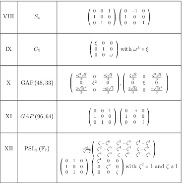
In 1976 Henn gives the next classification up to C− isomorphism of the non-singular plane quartic curves:
Case Model Aut(C) PM
I x4+x2F(y, z) +G(y, z) C
2 F(y, z) ≠0, not below
II x4+y4+z4+ax2y2+by2z2+cz2x2 V
4 a≠ ±b≠c≠ ±a
III z3y+x(x−y) (x−ay) (x−by) C
3 not below
IV x3z+y3z+x2y2+axyz2+bz4 S
3 a≠b and ab≠0
V x4+y4+z4+ax2y2+bxyz2 D
4 b≠0, ±√2a
1−a
VI z3y+x4+ax2y2+y4 C
6 a≠0
VII x4+y4+z4+ax2y2 GAP(16,13) ±a≠0,2,6,2√−3
VIII x4+y4+z4+a(x2y2+y2z2+z2x2) S
4 a≠0, −1±
√ −7
2
IX x4+xy3+yz3 C
9
-X x4+y4+xz3 GAP(48,33)
-XI x4+y4+z4 GAP(96,64)
-XII x3y+y3z+z3x PSL
2(F7)
-Where P M means parameter restrictions and “not below” means not C−isomorphic to any model below.
In table (5.1) of the Apendix 3, generators of each of these automorphism groups are given. Now, we show an example of a plane quartic curve defined over Q such that its reprensentative in Henn’s classification is not defined over Q: the quartic curve 5x4+y4+ z4+x2y2 = 0 that belongs to the case VII has as representative the curve with parameter a=1/√5. Moreover, notice that the representative does not have to be unique, in the former case we can take also a= −1/√5.
2.2. MODIFIED HENN CLASSIFICATION 23
Theorem 2.1.1. (Weil’s restriction principle) Let C/F be a curve defined over a number field F which is an extension F/k, then the curve C/F admits a model C′ defined over k
if and only if for all σ ∈ Gal(F˜/k), where F˜ is the Galois clousure of F/k, there exists an isomorphism φσ ∶ σC → C defined over F˜ and such that for all τ ∈ Gal(F˜/k) one has φστ =φσσφτ.
The idea of the proof, that will be useful in the following, is that if there is an isomorphism φ∶ C′→C, then we can define φ
σ=φσφ−1 for allσ∈Gal(F˜/k)and the relation φστ =φσσφτ
is satisfied for all σ, τ ∈Gal(F˜/k). Conversely, if we assume that C and C′ are canonical
curves, given a familly of isomorphismsφσ such that the relationφστ =φσσφτ holds, Hilbert’s
90th Problem states that is possible to find an isomorphism φ∶ C′→C such thatφ
σ=φσφ−1
for all σ∈Gal(F˜/k).
Dixmier-Ohno invariants
For elliptic curves the j− invariants allow us to determine when given two elliptic curves they are isomorphic. For genus two curves the Igusa invariants play this role. And for non-hyperelliptic genus three curves we have the absolute Dixmier-Ohno invariants. In [25] there is a survey about the topic.
Theorem 2.1.2. (Dixmier-Ohno) Two plane quartic curves are isomorphic if and only if they have the same absolute Dixmier-Ohno invariants.
Remark 2.1.3. If a plane quartic curve is defined over a number field k, then its absolute invariants of Dixmier-Ohno are also defined over k. But, the converse is not true.
Girard, Kohel and Ritzenthaler have implemented an algorithm in SAGE for computing the absolute Dixmier-Ohno invariants of a plane quartic curve, even if such curve is given by parameters, [26].
2.2
Modified Henn classification
Since cases IX, X, XI, XII are already defined over Q, we have just to study the cases from I to VIII. Let F be a number field, and let C/F be a plane quartic curve given by its Henn model and such that it belongs to the cases I, III, IV, V, VI or VII. Then its automorphisms group is given by projective matrices (after a suitable permutation of the variables):
⎛ ⎜ ⎝
∗ ∗ 0 ∗ ∗ 0 0 0 1
Assume that C/F is isomorphic to another curve C′ defined over a subextension k ⊆ F.
Then, by Weil restriction Principle, for all σ∈Gk there exists an isomorphism φσ ∶ σC →C,
that we can see as a projective matrix. Then we have that φ−1
σ Aut(C)φσ =Aut(σC). So, in
particular (check the eigenvalues or the elements in the center of Aut(C)): φ−1
σ Aφσ=B,
where:
Case A B
I
⎛
⎜
⎝
−1 0 0
0 −1 0
0 0 1
⎞ ⎟ ⎠ ⎛ ⎜ ⎝
−1 0 0
0 −1 0
0 0 1
⎞ ⎟ ⎠ III ⎛ ⎜ ⎝
ζ3 0 0
0 ζ3 0
0 0 1
⎞ ⎟ ⎠ ⎛ ⎜ ⎝
ζ3 0 0
0 ζ3 0
0 0 1
⎞ ⎟ ⎠ IV ⎛ ⎜ ⎝
ζ3 0 0
0 ζ2 3 0
0 0 1
⎞ ⎟ ⎠ ⎛ ⎜ ⎝
ζ3 0 0
0 ζ2 3 0
0 0 1
⎞
⎟
⎠
α
whereα=1,2
V
⎛
⎜
⎝
−1 0 0
0 −1 0
0 0 1
⎞ ⎟ ⎠ ⎛ ⎜ ⎝
−1 0 0
0 −1 0
0 0 1
⎞ ⎟ ⎠ VI ⎛ ⎜ ⎝
−1 0 0
0 1 0
0 0 ζ3
⎞ ⎟ ⎠ ⎛ ⎜ ⎝
−1 0 0
0 1 0
0 0 ζ3
⎞ ⎟ ⎠ VII ⎛ ⎜ ⎝
i 0 0 0 i 0 0 0 1
⎞ ⎟ ⎠ ⎛ ⎜ ⎝
i 0 0 0 i 0 0 0 1
⎞
⎟
⎠
α
2.2. MODIFIED HENN CLASSIFICATION 25
A case by case computation shows that:
φσ = ⎛ ⎜ ⎝
∗ ∗ 0 ∗ ∗ 0 0 0 1
⎞ ⎟ ⎠.
And, in the case VI, moreover we deduce that φσ has to be a diagonal matrix.
Case I
Here, C ∶ z4+F(x, y)z2+G(x, y) =0 is defined over F and we assume that there is a model C′ of C defined over a subextension F/k. Since we know that for all σ∈G
k:
φσ = ⎛ ⎜ ⎝
∗ ∗ 0 ∗ ∗ 0 0 0 1
⎞ ⎟ ⎠,
we can take the φin the idea of the proof of the Weil’s restriction principle also in the form, see remark (1.3.3):
φ=⎛⎜ ⎝
∗ ∗ 0 ∗ ∗ 0 0 0 1
⎞ ⎟ ⎠.
And then, C′ ∶ z4 +F′(x, y)z2 +G′(x, y) = 0, so the family for this strata in the Henn
classification was alredy complete.
Case II
After a suitable change of coordinates we can work with the model C∶ ax4+by4+cz4+x2y2+ y2z2+z2x2 = 0. Let σ ∈Gal(F˜/k) be such that the conjugation by φ
σ on Aut(C) leaves a
non trivial automorphism fixed. Then we can assume that:
φσ= ⎛ ⎜ ⎝
α β 0
γ δ 0 0 0 1
⎞ ⎟ ⎠∶
σC →C.
Then, it is easy to check that σc=cand σa=a and σb=b or σa=b and σb=a. If φ σ only
leaves fixed the trivial automorphism, then it is easy to check again that we can assume:
φσ = ⎛ ⎜ ⎝
0 α 0 0 0 β
γ 0 0
And then α2 = 1/β2 = γ2 =1/α2. So, σa = c, σb =a and σc=b. Hence, in any case a, b, c
are the roots of a degree 3 polynomial with coefficients in k. And then we can consider the model:
C′∶ (x+ay+a2z)4+ (x+by+b2z)4+ (x+cy+c2z)4+ (x+ay+a2z)2(x+by+b2z)2+
+(x+by+b2z)2(x+cy+c2z)2+ (x+cy+c2z)2(x+ay+a2z)2=0 (2.1)
given by the isomorphism:
φ=⎛⎜ ⎝
1 a a2
1 b b2
1 c c2 ⎞ ⎟ ⎠∶ C
′→
C.
Case III
We have C∶ z3y+x(x−y)(x−a)(x−b) =0, and we can take theφ in the idea of the proof
of the Weil’s restriction principle of the form:
φ=⎛⎜ ⎝
α β 0
γ δ 0 0 0 1
⎞ ⎟ ⎠.
And then we get the equation z3(γx+δy) +Q(x, y) = 0 where Q(x, y) is an homogenous
degree 4 polynomial in x and y. Since that equation is defined over k, then δ/γ∈k. Hence, we can do the change of variables x′ =x and y′ =γx+δy and then we get the k−rational
model C′∶ z3y+P(x, y) =0.
Case IV
We start with the variation of the Henn’s model C ∶ z4+axyz2+b(x3+y3)z+x2y2 =0. In
this case again:
φσ = ⎛ ⎜ ⎝
∗ ∗ 0 ∗ ∗ 0 0 0 1
⎞ ⎟ ⎠. Then, we can take:
φ=⎛⎜ ⎝
α β 0
γ δ 0 0 0 1
⎞ ⎟ ⎠.
And then, if we get an equation of C′ from the equation of C and the isomorphism φ, we
conclude:
2.2. MODIFIED HENN CLASSIFICATION 27
So, after maybe permuting the variables xand y we can assumeβ=γ=0 and then δ= ±1/α and σa= ±a. If we look at the coefficient of degree 1 inz of the equation ofC′, we conclude
α3 =i, where =0,1,2 or 3. And then σb=ib. Hence, there exist k−rational numbers m, q
such that b=√4 m and a=q√m. After dividing z by √4 m we obtain the rational model:
C′∶
z4/m+qxyz2+ (x3+y3)z+x2y2=0.
So the family for this strata in the Henn classification was alredy complete.
Case V
In that case C ∶ x4+y4+z4+ax2y2+bxyz2. Let
φσ = ⎛ ⎜ ⎝
α β 0
γ δ 0
0 0 1 ⎞ ⎟ ⎠.
Then, x4 +y4 +z4 + σax2y2 + σbxyz2 = (αx +βy)4 + (γx+δy)4 +z4 +a(αx+βy)2(γx+ δy)2+b(αx+βy)(γx+δy)z2. If we look at the coefficient of xyz2 in the left hand side: σbxyz2 =b(αx+βy)(γx+δy)z2, and then, after maybe permuting the variables x, y we can
assume β = γ = 0. So, α4 = δ4 = 1 and then σa = ±a and σb = ib, where = 0,1,2 or 3.
Hence, there exist k−rational numbers m, q such that: b= √4 m and a =q√m. We find the
k−rational model: C′∶ 1/mx4+y4+z4+qx2y2+xyz2 =0 and the isomorphism:
φ=⎛⎜ ⎝
4
√
m3 0 0
0 m 0
0 0 m
⎞ ⎟ ⎠∶ C
′→
C.
Case VI
We have the plane quartic C∶ z3y+x4+ax2y2+y4 =0, and since the automorphism group
in this case is made up of diagonal matrices, we can take
φσ = ⎛ ⎜ ⎝
α 0 0 0 1 0 0 0 β
⎞ ⎟ ⎠.
Then α4 =1 and σa= ±a. So, there exists a k−rational number m such that a=√m. And
after dividing x by √4
m we obtain the k−rational model: C′∶ z3y+1/mx4+x2y2+y4=0.
Caso VII
In this case we have C∶ x4+y4+z4+ax2y2. Let again
φσ = ⎛ ⎜ ⎝
α β 0
γ δ 0 0 0 1
⎞ ⎟ ⎠
be an isomorphism φσ∶ σC→C. Then,
α4+γ4+aα2γ2 =1
4α3β+4γ3δ+a(2α2γδ+2αβγ2) =0
6α2β2+6γ2δ+
a(α2δ2+β2γ2+4αβγδ) = σa
4αβ3+4γδ3+a(2β2γδ+2αβδ2) =0
β4+δ4+aβ2δ2 =1
If we subtract βδ times the second equation to αγ times the fourth one, we get γδ = ±αβ. If we plug this condition into the second equation we get αβ =0 or α2 = ±γ2. The
second condition gives to us k−rational values of a, while the first one gives σa= ±a. Then, C ∶ x4+y4 +z4 +√mx2y2 = 0 for some m ∈ k. And we find the k−rational model: C′ ∶
x4/m+y4+z4+x2y2=0 via the isomorphism:
φ=⎛⎜ ⎝
1/√4 m 0 0
0 1 0
0 0 1
⎞ ⎟ ⎠∶ C
′→
C.
Case VIII
In this case the previous arguments do not work. We will use here the Dixmier-Ohno invariants that are computed in table (5.4). If C ∶ x4+y4+z4+a(x2y2+y2z2+z2x2) =0 is
isomorphic to curve defined overk then its Dixmier-Ohno invariants are also defined over k. We will prove that in this case, necersarly we have a∈k. We have the following relations:
q∶= I9 I12 = (
a+3)(a+18) a2−9a−6 ∈k,
q′∶= I18
I12
I15
I27 =
2.3. A REPRESENTATIVE IN THE MODIFIED HENN CLASSIFICATION 29
If a ∈k we are done, then lets us assume that a∉k and then it is in a quadratic extension of k. Hence, the two equations above should be one a multiple of the other, both give the minimal polynomial of a over k. We get q= 12 or −52, and then 4 possible values of a. If we plug these values in the other invariants we do not get k−rational numbers. Then a∈k and the family for this strata in the Henn classification is alredy complete.
We summarize all the previous results in next table. In table (5.2), generators of each of these automorphism groups are given.
Case Model Aut(C) PM
I x4+x2F (y, z) +G(y, z) C
2 F (y, z) ≠0, not below
II see 2.1 V4 a≠b≠c≠a
III z3y+P(x, y) C
3 not below
IV x3z+y3z+x2y2+axyz2+bz4 S
3 a≠b and ab≠0
V ax4+y4+z4+bx2y2+xyz2 D
4 b≠0, a≠4b2(2b+1)2
VI z3y+ax4+x2y2+y4 C
6
-VII ax4+y4+z4+x2y2 GAP(16,13) ±a≠1/4,1/36,1/ −12
VIII x4+y4+z4+a(x2y2+y2z2+z2x2) S
4 a≠0, −1±
√ −7
2
IX x4+xy3+yz3 C
9
-X x4+y4+xz3 GAP(48,33)
-XI x4+y4+z4 GAP(96,64)
-XII x3y+y3z+z3x PSL
2(F7)
-Table 2.2: Modified Henn classification
2.3
A representative in the modified Henn
classifica-tion
Let C/k be a plane quartic curve. Assume that the automorphism group Aut(C) is non-trivial and known, and given by proyective matrices. We will show how to find a Henn model CH of C, that is a representative of this curve in the Henn classification, and an
then Aut(CH) =ϕAut(C)ϕ−1. So, the idea will be find a projective matrix ϕsuch that the
last equality holds.
Case I
In that case there is only one non-trivial automorphism α ∈Aut(C). The automorphism α is similar to the matrix:
⎛ ⎜ ⎝
−1 0 0 0 1 0 0 0 1
⎞ ⎟ ⎠.
Find the eigenvector v1 of the projective matrix α corresponding to the eigenvalue that is
different from the other two and two eigenvectors v2 andv3 corresponding to these two equal
eigenvalues, then
ϕ−1 = (
v1∣λ1v2+λ2v3∣λ3v2+λ4v3).
Get the equation of CH via this ϕ and the equation of C and adjust the scalars λ1, λ2, λ3
and λ4 for getting CH defined over k.
Case II
Each of the 3 non-trivial automorphisms in Aut(C) diagonalize simultaneously into: ⎛
⎜ ⎝
−1 0 0 0 1 0 0 0 1
⎞ ⎟ ⎠, ⎛ ⎜ ⎝
1 0 0 0 −1 0 0 0 1
⎞ ⎟ ⎠, ⎛ ⎜ ⎝
1 0 0 0 1 0 0 0 −1
⎞ ⎟ ⎠.
Letvifori=1,2,3 the eigenvector corresponding to the eigenvalue−1 for each automorphism.
Then
ϕ−1= (
v1 ∣λ1v2∣λ2v3).
Now, get the equation ofCH via thisϕand the equation ofC; and adjust the scalarsλ1 and λ2 for getting CH defined over k.
Example 2.3.1. Let be
C∶ 3x4+10x2y2+5x2z2−2xyz2+3y4+5y2z2+z4 =0,
the automorphism group Aut(C) is generated by the matrices:
⎛ ⎜ ⎝
1 0 0 0 1 0 0 0 −1
⎞ ⎟ ⎠, ⎛ ⎜ ⎝
0 1 0 1 0 0 0 0 1
2.3. A REPRESENTATIVE IN THE MODIFIED HENN CLASSIFICATION 31
For the first one we obtain the eigenvector with eigenvalue −1: (0 ∶ 0 ∶ 1), the other two eigenvalues are equal to 1. For the second one we obtain (1∶ −1∶0) with eigenvalue equal to
−1, the other two eigenvalues are equal to 1. The other non-trivial automorphism is
⎛ ⎜ ⎝
0 1 0 1 0 0 0 0 −1
⎞ ⎟ ⎠.
and we find (1∶1∶0) with eigenvalue equal to 1, the other two eigenvalues are equal to −1. Then the isomorphism ϕ−1 ∶ C
H →C is given by:
ϕ−1=⎛⎜
⎝
λ1 λ2 0 −λ1 λ2 0
0 0 1
⎞ ⎟ ⎠.
We subtitute in the equation of C for getting an equation of CH:
CH ∶ 16λ41x4+16λ42y4+z4+16λ21λ22x2y2+8λ22y2z2+12λ21z2x2 =0.
Then λ2 1 =
±1
4 = λ 2
2, and hence, a = 1, b = 2 and c = 3 (in case II of Henn classification
multiplying a parameter by −1 gives us the same quartic curve up to isomorphism). Finally,
CH ∶ x4+y4+z4+x2y2+2y2z2+3z2x2=0.
Case III
In that case we proceed as in the case I but considering the automorphism: ⎛
⎜ ⎝
1 0 0 0 1 0 0 0 ξ3
⎞ ⎟ ⎠.
Cases from IV to VII and from IX to XII
Find a matrix in Aut(C) such that is similar to M (see the table above). Next, find the eigenvectors corresponding to the different eigenvalues: v1, v2,v3. Then
ϕ−1= (
v1 ∣λ1v2∣λ2v3).
Finally, get the equation of CH via this ϕ−1 and the equation of C and adjust the scalarsλ1
Case M
IV
⎛
⎜
⎝
ξ3 0 0
0 ξ2 3 0
0 0 1
⎞ ⎟ ⎠ V ⎛ ⎜ ⎝
i 0 0 0 −i 0
0 0 1
⎞ ⎟ ⎠ VI ⎛ ⎜ ⎝
−1 0 0
0 1 0
0 0 ξ3
⎞ ⎟ ⎠ VII ⎛ ⎜ ⎝
i 0 0 0 −i 0
0 0 1
⎞ ⎟ ⎠ IX ⎛ ⎜ ⎝
ξ3 0 0
0 1 0 0 0 ξ9
⎞ ⎟ ⎠ X ⎛ ⎜ ⎝
1 0 0 0 i 0 0 0 ξ3
⎞ ⎟ ⎠ XI ⎛ ⎜ ⎝
i 0 0 0 −i 0
0 0 1
⎞ ⎟ ⎠ XII ⎛ ⎜ ⎝ ξ4
7 0 0
0 ξ2 7 0
0 0 ξ7
⎞
⎟
2.3. A REPRESENTATIVE IN THE MODIFIED HENN CLASSIFICATION 33
Case VIII
We proceed as in the case II with the subgroup of Aut(C)generated by the matrices: ⎛
⎜ ⎝
1 0 0 0 1 0 0 0 −1
⎞ ⎟ ⎠,
⎛ ⎜ ⎝
−1 0 0 0 1 0 0 0 1
⎞ ⎟ ⎠.
Finally, given a plane quartic curveC/F such that Aut(C)is known, we can find its Henn modelCH/kwithk⊆F the minimal field over which a curve isomorphic toCis defined. And
we will be able of computing its twists looking at the results that we obtain in chapter 3, that is, the computation of the twists of the quartic curves in the modified Henn classification.
Chapter 3
Twists of non-hyperelliptic genus
3
curves
In this chapter we compute the twists of each representative in the families of the modified Henn classification over a number field k. There are some cases in which all the machinery developed in chapter 1 is not needed. Firstly, we will deal with the case of the twists of the Fermat quartic, a difficult case for which we need all the tools in chapter 1. Then, we will compute the twists of cases from I to X. For the cases II, V, VII and VIII we will use the knowledge about the twists of the Fermat quartic. The other cases will be done just inspeccioning the form of the equations using remark (1.3.3) and we will use remark (1.3.1) for checking when they are equivalent. Finally, case XII, the case of the Klein quartic, the more difficult one, will be done using again the machinery in chapter 1. This case becomes so hard because the Galois embedding problems that appear are difficult to solve.
3.1
The Fermat quartic
We consider the Fermat quartic CF ∶ x4+y4+z4 = 0 defined over a number field k. The
automorphism group Aut(CF) is isomorphic to < 96,64 > in GAP notation [24], and as
subgroup of PGL3(¯k) it is generated by the matrices:
s=⎛⎜ ⎝
0 0 1 1 0 0 0 1 0
⎞ ⎟
⎠, t= ⎛ ⎜ ⎝
0 −1 0 1 0 0 0 0 1
⎞ ⎟
⎠, u= ⎛ ⎜ ⎝
i 0 0 0 1 0 0 0 1
⎞ ⎟ ⎠
Let us firstly suppose that i∉k, then K =k(i), Gal(K/k) ≃Z/2Z and Γ=Aut(CF) ⋊
Gal(K/k) ≃< 192,956 >. Then, it is easily checked with MAGMA [6], see the code in table (5.5) in the appendix, that the possible pairs (G, H) in (1.3) are the ones given in the tables below. We have divided these pairs into three types: diagonal, almost diagonal
and non-diagonal. The diagonal type corresponds to the cases in which all the elements in G⊆Aut(CF) ⋊Gal(K/k) have a diagonal matrix as first component. The second type will
be called almost-diagonal and it corresponds to the cases where Gis a 2-group not included in the diagonal cases of the former type. Finally, the third type will cover the pairs (G, H) of the remaining cases.
In the tables below the fourth and fifth columns serve to reconstruct G and H. The fourth column contains a list of generators of H, and the fifth column contains a single matrix h. The meaning is that G is the group which elements are (g,1)for g inH together with the elements (gh, τ) for g in H and τ the non-trivial automorphism in Gal(K/k). As an easy way to remember, we can write the non-sense expression G=H⋊1+Hh⋊τ.
Type I: Diagonal twists
ID(G) ID(H) gen(H) h 1 <2,1> <1,1> 1 1 2 <2,1> <1,1> 1 t3utu
3 <4,2> <2,1> t2 1
4 <4,2> <2,1> t2 u
5 <4,2> <2,1> t2 t3utu
6 <8,5> <4,2> t2, u2 1
7 <8,5> <4,2> t2, u2 u
8 <8,3> <4,1> t3utu 1
9 <8,3> <4,1> t3utu u
10 <8,3> <4,1> t3utu3 1
11 <8,3> <4,1> t3utu3 u
12 <16,11> <8,2> t3utu, u2 1
13 <16,11> <8,2> t3utu, u2 u
14 <32,34> <16,2> u, t3ut 1
Type II: Almost-diagonal twists ID(G) ID(H) gen(H) h 1 <2,1> <1,1> 1 u2t
2 <4,2> <2,1> t2 u2t
3 <4,1> <2,1> t2 t
4 <4,2> <2,1> u2t 1
5 <4,2> <2,1> u2t t3utu
6 <8,4> <4,1> t3utu t