OPTIMIZATION METHODS FOR THE ITERATIVE SOLUTION OF COUPLED FLUID-STRUCTURAL PROBLEMS

OPTIMIZATION METHODS FOR THE ITERATIVE SOLUTION

OF COUPLED FLUID-STRUCTURAL PROBLEMS

PACS REFERENCE: 43.55.Ka

Franck, Andreas

Institute of Technical Acoustics Aachen University (RWTH) 52056 Aachen

Germany

Tel: +49-241-8097998 Fax: +49-241-8092214

E-mail: Andreas.Franck@akustik.rwth-aachen.de

ABSTRACT

The finite element modeling of coupled fluid-structural problems, arising e.g. from the coupled simulation of room acoustical and building acoustical problems, leads to large sparse unsymmet-ric linear systems of equations. Due to the size of the system matunsymmet-rices, an iterative solution is appropriate.

For the typical case of weak coupling between fluid and structure, the calculation of the cou-pled system can eventually be accelerated by a decoupling approach, using the solutions of the decoupled symmetric systems as starting points for the solution of the coupled unsymmetric sys-tem. This decoupling enables the use of the more powerful optimization techniques for symmetric problems.

INTRODUCTION

The Finite Element Method (FEM) is a standard method for the simulation of sound fields in enclosures. Using a volume discretization and a variational approach, this numerical method finds approximate solutions of the Helmholtz equation.

The proper modeling of the impedance boundary conditions of real walls is not possible with this approach however, when the walls cannot be regarded as locally reacting. So, the excitation of natural oscillations of wall structures introduces additional errors. For an accurate simulation the effects of fluid-structural coupling have to be taken into account.

FINITE ELEMENT MODELS FOR FLUID AND STRUCTURE

Fluid Model

In the frequency domain, the acoustical wave propagation in fluid media is described by the Helmholtz equation

∆p+k2p= 0 ∀~r∈Ω withk=ω

and its associated boundary conditions, which can be formulated as the admittance boundary condition for absorbing walls

∇p·~n= ∂p

∂~n =−jωρAnpn ∀~r∈ΓA (2)

and the velocity boundary condition for sources (vibrating panels)

∇p·~n= ∂p

∂~n =−jωρvn ∀~r∈Γv . (3)

In this discussion, all non-vibrating boundaries will be regarded as rigid (An= 0).

Analytical solutions of the Helmholtz equation can only be obtained for very simple enclosure geometries. So, to be able to accurately calculate the sound field in arbitrary shaped enclosures, one has to resort to numerical methods. One of the most widely known methods for this purpose is the Finite Element Method (FEM) [4, 6].

Using a variational approach and discretizing the enclosure volume with 3D finite elements, the Finite Element Method is able to calculate approximate solution to the Helmholtz equation [2]. So, this solutions are obtained by solving the linear system of equations inp:

SF−ω2MF

p=j ωBFvn (4)

whereω is the angular frequency, SF the acoustical stiffness matrix, MF the acoustical mass

matrix, and BF an interpolation matrix for the normal surface velocity vn given at the surface

nodes.

Structural Model

With a variational approach involving the deformation energy and the energy due to the acceler-ation of the distributed mass, the vibracceler-ation behavior of an elastic structure can also be calculated using a Finite Element Model [4, 6].

Ignoring the damping and nonlinearities, the Finite Element system of equations for an elastic structure takes the form

SS−ω2MSu=GSg+F (5)

where againω is the angular frequency, uis the vector of the unknown displacements (having 3 degrees of freedom for each node), SS is the structural stiffness matrix (depending on the

E modulus and the Poisson numberν),MS is the structural mass matrix (depending on the mass

densityρ),GS is an interpolation matrix for the surface pressure stimulusg, andFis a vector of

point force stimuli.

COUPLED FLUID-STRUCTURAL FE MODEL

On the boundary between fluid and structure, two coupling mechanisms must be taken into ac-count. First, the vibrating surface of the structure will radiate sound into the fluid medium. Second, a sound field within the fluid medium will excite structural vibrations due to the sound pressure on the structure surface.

WithnF as the surface normal vector pointing from the fluid volume into the structure volume and

nS=−nF, this coupling conditions can be formulated as

jω˜vn=ω2u·nS =−ω2u·nF (6)

for the radiation of sound due to the structural surface vibrations and

˜

S

F y

n

x ~

~

Fluid

u

u

n

n

v

p

g

Structure

Figure 1: Coupling conditions at the fluid-structure boundary

for the excitation of structural vibrations due to a sound field in the fluid medium.

Again, this coupling conditions can be expressed in the Finite Element model as

GS˜g = −KSp (8)

j ωBFv˜n = ω2KFu (9)

where˜vnis the additional surface velocity for the fluid model and˜gis an additional surface

pres-sure vector for the structural model.

Substituting the coupling conditions into the previously introduced FE systems for the fluid and the structure results in two coupled systems of equations:

SS−ω2MS

u = GSg+F−KSp (10)

SF−ω2MF

p = j ωBFvn+ω2KFu. (11)

which can be rewritten as

    

SS KS

0 SF

| {z }

SC

−ω2

MS 0

KF MF

| {z }

MC

    

u p

| {z }

xC

=

TSf+GSg+F

j ωBFvn

| {z }

bC

(12)

with the unsymmetric system matricesSCandMC.

SOLUTION TECHNIQUES

In the currently implemented state of the solver, the symmetric systems (4) and (5) are solved by a preconditioned conjugate gradient (PCG) algorithm [5]. For each iteration step of CG, most of the processing time is spent in the computation of the matrix-vector product

q← S−ω2M

p. (13)

Figure 2: Simple example of a coupled fluid-structural model

an extension to the CG algorithm is suitable, which is widely known as the biconjugate gradient method (BiCG) [1, 5].

Being based on the conjugate gradient method, the BiCG algorithm still spends most of its com-putation time per iteration in the calculation of matrix-vector products, but in contrast to the CG algorithm, two matrix-vector products are needed in each iteration step:

q ← SC−ω2MCp (14)

˜

q ← SC−ω2MC

T ˜

p. (15)

So, even when a coupled solution can be obtained in the same number of iteration steps as an uncoupled solution of the same system (e.g., withKS =KF = 0), a coupled solution using the

BiCG method will take about twice the computation time.

The model shown in Figure 2 consists of a thin plate on one wall of an otherwise rigidly bounded cubic enclosure. It was discretized with 1856 structural tetrahedron elements of second order and 6232 fluid tetrahedron elements of second order, leading to a matrix dimension of 22039 degrees of freedom. A surface-normal point force on the exterior plate surface was used to excite structural vibrations of the plate. A point source with constant volume velocity within the fluid volume was used to excite a sound field in the fluid.

For this model, the iteration counts and computation times for an uncoupled (CG) and a coupled (BiCG) simulation are shown in Table 1.

f [Hz] 31.5 63 125 250 500

n(CG solver, structural stimulus) 1065 1065 1068 1082 1345

n(BiCG solver, structural stimulus) 1142 1187 1196 1939 4061

T [s] (CG solver, structural stimulus) 57.41 58.24 58.02 58.85 72.02

T [s] (BiCG solver, structural stimulus) 125.42 130.49 130.90 213.28 449.33

n(CG solver, fluid stimulus) 285 283 299 466 935

n(BiCG solver, fluid stimulus) 1199 1158 1183 1742 3911

T [s] (CG solver, fluid stimulus) 15.21 15.06 16.60 24.77 50.63

T [s] (BiCG solver, fluid stimulus) 131.68 127.09 132.69 204.30 439.93

n(CG solver, both stimuli) 1242 1254 1242 2265 3940

n(BiCG solver, both stiumuli) 1265 1237 1421 2322 4526

T [s] (CG solver, both stimuli) 70.00 66.79 66.05 122.29 208.90

T [s] (BiCG solver, both stimuli) 141.46 139.17 158.23 263.32 502.31

Table 1: Comparison between coupled and uncoupled simulations

Examining the solutions, it can be noted that the structure displacements due to a structural excitation are nearly identical, regardless of the consideration of coupling effects. This is due to the relatively weak coupling between fluid and structure - the radiated sound field of the structure has only a very small reverse effect on the structural vibration.

Now, an approach based on this observation will be discussed to eventually allow faster compu-tations, while still preserving the possibility to consider the coupling with a reasonable accuracy.

PROPOSED OPTIMIZATION APPROACH

Using the CG solver, it is possible to obtain a solution

u(0)_,p(0)T

of the uncoupled system

SS 0

0 SF

−ω2

MS 0

0 MF

u(0)

p(0)

=

TSf+GSg+F

j ωBFvn

. (16)

Using the relations from (10) and (11), further approximations to a coupled solution can be ob-tained by introducing additional excitation terms on the right hand side of the system:

SS 0

0 SF

−ω2

MS 0

0 MF

u(m+1)

p(m+1)

=

TSf+GSg+F

j ωBFvn

+

−KSp(m)

ω2_K Fu(m)

(17)

Due to the symmetry of this systems, they can be solved using algorithms for symmetric problems, avoiding the higher costs of an unsymmetric solver like BiCG. Using some steps of the iteration (17) (called solution update in the further discussion), a very good approximation to a coupled solution can be obtained. Furthermore, it is possible to adjust the accuracy of the needed solution by limiting the number of solution updates. Finally, one of the approximate solutions can be used as the starting point for a fully coupled solution using BiCG.

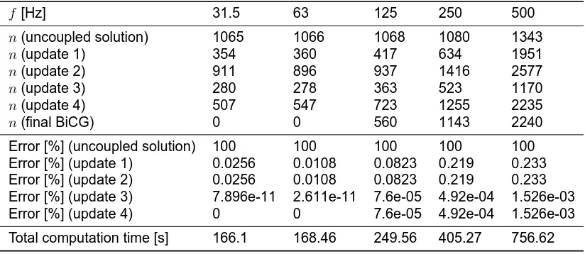
For the introduced example, using a force on the structure surface this approach has been tested. The uncoupled solution was taken as a starting point, and four solution update steps were per-formed. After the last solution update, the BiCG solver was used to finally calculate the coupled solution, and the numerical error of each intermediate solution (relative to the coupled BiCG so-lution) was analyzed.

f [Hz] 31.5 63 125 250 500

n(uncoupled solution) 1065 1066 1068 1080 1343

n(update 1) 354 360 417 634 1951

n(update 2) 911 896 937 1416 2577

n(update 3) 280 278 363 523 1170

n(update 4) 507 547 723 1255 2235

n(final BiCG) 0 0 560 1143 2240

Error [%] (uncoupled solution) 100 100 100 100 100 Error [%] (update 1) 0.0256 0.0108 0.0823 0.219 0.233 Error [%] (update 2) 0.0256 0.0108 0.0823 0.219 0.233 Error [%] (update 3) 7.896e-11 2.611e-11 7.6e-05 4.92e-04 1.526e-03 Error [%] (update 4) 0 0 7.6e-05 4.92e-04 1.526e-03

Total computation time [s] 166.1 168.46 249.56 405.27 756.62

Table 2: Results for the suggested solution update scheme

The first update has a large effect on the error because the uncoupled has a zero sound field in the fluid medium in this case. With a few update steps, the error can be reduced even further. So, for the two lowest frequencies, four update steps were sufficient to lower the residual so far, that the BiCG solver needed no further iterations to converge.

matrix-vector products then is usually higher than for a fully coupled BiCG simulation, resulting in longer computation times. But the proposed scheme might be beneficial in two special cases: first, when an uncoupled solution has to be calculated anyways, or is previously available, or second, when a limited accuracy for the bidirectional coupling is sufficient.

CONCLUSIONS

It has been shown that it is possible to calculate the solution of coupled fluid-structural problems without having to solve an unsymmetric system of equations. It is possible to control the accuracy of the coupled solutions, thereby reducing the computation time if no full-precision solution is required or if uncoupled solutions are previously available.

However, there is no overall benefit over a BiCG solver, which, using proper preconditioning, can obtain a coupled solution faster than the proposed solution-update technique. So, the focus for further optimizations should concentrate on improvements within the BiCG solver, for example by taking special measures to exploit the system matrix structure or by calculating the two matrix-vector products at once, thereby reducing the per-iteration computation time [3].

REFERENCES

[1] R. Barrett, M. Berry, T. F. Chan, J. Demmel, J. Donato, J. Dongarra, V. Eijkhout, R. Pozo, C. Romine, and H. Van der Vorst. Templates for the Solution of Linear Systems: Building

Blocks for Iterative Methods. SIAM, Philadelphia, PA, 2. edition, 1994.

[2] Guido Bartsch. A simulation package for room acoustics with an open interface. In Proc.

137th ASA / 2nd EAA / Forum Acusticum Meeting, Berlin, Germany, 1999.

[3] Guido Bartsch and Andreas Franck. A hybrid and parallel extension of the sound field simu-lation for interior problems. In Proceedings of the 7th International Congress on Sound and

Vibration (ICSV), Garmisch-Partenkirchen, Germany, 2000.

[4] Klaus-J ¨urgen Bathe. Finite-Elemente-Methoden. Springer-Verlag, Berlin, Heidelberg, New York, Tokyo, 1986.

[5] Gene H. Golub and Charles F. van Loan. Matrix Computations. The John Hopkins University Press, Baltimore, London, 3. edition, 1996.