USING STATED PREFERENCE TO VALUE NOISE FROM AIRCRAFT IN THREE EUROPEAN COUNTRIES

(1)

G

Guuiimmaarrããeess--PPoorrttuuggaall

paper ID:013/p.1

USING STATED PREFERENCE TO VALUE NOISE

FROM AIRCRAFT IN THREE EUROPEAN COUNTRIES

M. Wardman

a

and A.L. Bristow

a

a _{Institute for Transport Studies,University of Leeds, Leeds, England, mwardman@its.leeds.ac.uk}

ABSTRACT: This paper reports results from three novel Stated Preference exercises conducted at Manchester, Lyon and Bucharest Airports. It finds that masking the purpose of the exercise produces lower values of aircraft noise than where the purpose of the study is clear. Whilst values split by time period also seem far too high, due to incentives to bias responses, their relativities seem reasonable and provide a means of disaggregating overall values.

1. INTRODUCTION

This paper reports novel applications of Stated Preference (SP) to the valuation of aircraft noise. The research was wide ranging in nature, covering as it does two forms of SP method, contrasting incentives to response bias, differing levels of time period disaggregation and the three airports of Manchester, Lyon and Bucharest. After outlining the methodology in section 2, we present the aircraft noise valuations from three SP exercises in the section 3. Section 4 compares the results from the different exercises and concluding remarks are provided in section 5.

2. METHODOLOGY

Three SP exercises were used in this study. SP1 examined aircraft noise in a broader quality of life dimension alongside a wide range of other variables to mask the purpose of the study. SP2 is more conventional and based around trade-offs between aircraft noise and council tax in a specific time period. SP3 offered trade-offs between aircraft noise at different times of day. We here chose to proxy variations in noise by variations in aircraft movements, a measure which respondents ought to be able to relate to. These were defined as ‘planes going by’, and hence are half of the number of total movements. No distinction was made between take-offs and landings.

2.1 SP1

(2)

G

paper ID:013/p.2

[image:2.595.64.552.273.488.2]

nature of aircraft noise. Focus groups had revealed that aircraft noise naturally emerged in discussion of general quality of life. Table 1 illustrates the scenarios presented. The current position was established and then respondents identified the improvement that they would most like, followed by the second most preferred improvement and so on until all improvements were ranked in order of preference. The same procedure was then followed for deteriorations.

Table 1: Example of SP1 Exercise - Manchester (Cheadle Area)

Burglaries per 1000 Homes 10 5 2 1 0.5

Local Schools: % Pass Rate 10% 25% 40% 55% 70%

Area Traffic Congestion +10% +5% As Now -5% -10%

Street Cleanliness Very Dirty Dirty Neither Clean Very Clean

Traffic Noise at Home Extremely

Noisy Very Noisy Moderately Noisy Slightly Noisy

Not at all Noisy

Neighbourhood Air Quality Very Poor Poor Neither Good Very Good

Road/Pavement Condition Very Poor Poor Neither Good Very Good

Planes Go By Every 2m Day

Every 2m Eve

Every 4m Day Every 2m Eve

Every 4m Day Every 4m Eve

Every 4m Day Every 7½m Eve

Every 7½m Day Every 7½m Eve

Council Tax +£8 a

week

+£3 a week

+£1 a week

As Now -£1 a

week

-£3 a week

-£8 a week

No Library Library

Recreation Facilities

Locally Available _{No Sports/Leisure Facilities} _{Sports/Leisure Facilities}

No Local Food Shops Local Food Shops

Amenities Within Walking

Distance _{No Local Doctor} _{Local Doctor}

2.2 SP2

SP2 can be taken as a standard SP approach and offered eight choices between two alternatives characterised by council tax and aircraft movements. Aircraft movements were disaggregated into three plane types of large 4 engined planes, two engine jets and turbo-prop planes. In addition, respondents were asked to consider the variations in a specific time period, given that annoyance from aircraft will depend on the exposure to it and the activities being undertaken when the noise is experienced. The purpose of this exercise would have been quite transparent.

2.3 SP3

(3)

G

paper ID:013/p.3

Table 2: Example of SP3 Exercise – Manchester (Planes Per Hour)

Deteriorations Now Improvements

Every Weekday 6-9am 60 40 30 20 15 12 10

Every Weekday 9am-6pm 40 30 20 15 12 10 6

Every Weekday 6-10pm 30 20 15 12 10 6 4

Saturday 6-9am 60 40 30 20 15 12 10

Saturday 9am-6pm 40 30 20 15 12 10 6

Saturday 6-10pm 30 20 15 12 10 6 4

Sunday 9am-6pm 40 30 20 15 12 10 6

Every Night 6 4 3 2 1 0

Tax +£10 +£5 +£2 0 +£2 +£5 +£10

3. STATED PREFERENCE RESULTS

The surveys were conducted in late 2002 at six locations around each airport. Samples of 200 at Manchester, 210 at Lyon and 237 at Bucharest were obtained. The ALOGIT [1] package was used to estimate the relative importance attached to each attribute in each exercise and its jack-knife procedure accounted for individuals’ repeat observations. The ordered logit model was used to analyse the SP1 and SP3 data whilst the SP2 data was analysed using a standard logit model.

3.1 SP1 Results

[image:3.595.223.374.78.157.2]

Individuals who failed to rank the alternatives in logical order have been removed from the data set. This does not alter our conclusions but it does lead to more precise coefficient estimates. Table 3 reports the coefficients relating to aircraft movements and tax for both improvements and deteriorations. In both cases the models achieve goodness of fit measures (ρ2) in line with those typically achieved in more conventional SP choice models. A wide range of other statistically significant quality of life effects were also discerned at each location [2].

With regard to improvements, variations in daytime aircraft movements have a statistically significant effect in all three locations whilst evening aircraft movements have a significant effect in both Manchester and Lyon. Daytime values in Manchester and Lyon are similar, in line with their similar income levels, whilst the higher sensitivity of Lyon residents to evening aircraft noise was also apparent in the attitudinal responses. The lower incomes of Bucharest residents will at least in part explain their lower values.

(4)

G

paper ID:013/p.4

[image:4.595.69.521.237.398.2]

The value of increased aircraft movements is very much lower than reductions in Bucharest. This may reflect a ‘halo’ effect of perceived economic development associated with airport expansion.

Table 3: Results of SP1 Models

Manchester Lyon Bucharest

Coeff (t) Value (t) Coeff (t) Value (t) Coeff (t) Value (t)

Improvements

Aircraft: Day -0.139 (3.9) 1.08 (3.6) -0.170 (5.9) 0.91 (5.7) -0.669 (5.3) 0.48 (4.8)

Aircraft: Evening -0.053 (2.0) 0.41 (2.0) -0.244 (9.6) 1.31 (9.4) n.s

Tax (€) -0.129 (9.2) -0.186 (19.4) -1.399 (9.2)

ρ2

/individuals 0.106 109 0.097 130 0.109 67

Deteriorations

Aircraft: Day -0.062 (5.1) 0.81 (4.6) -0.083 (7.7) 1.28 (5.7) -0.085 (3.5) 0.03 (3.3)

Aircraft: Evening n.s -0.078 (7.1) 1.20 (5.9) n.s

Weekly Tax (€) -0.077 (8.3) -0.065 (8.6) -2.590 (9.8)

ρ2

/individuals 0.133 133 0.119 153 0.131 84

3.2 SP2 Results

[image:4.595.71.533.513.656.2]

The results for SP2 are reported in Table 4. The goodness of fit measures are low, particularly for Bucharest where respondents struggled more with the SP task, and they are lower than for SP1. However, the identification of irrational responses is not possible in this exercise. Due to the small samples sizes for some periods, it was not possible to obtain coefficients that were remotely significant for some time periods and these have been removed from the reported models.

Coeffs (t) Values (t) Coeffs (t) Values (t) Coeffs (t) Values (t) Constant-Quieter - 1.2899 (5.0) 26.11 (4.8) -1.2064 (6.4) -3.77 (6.3) Flights - Weekday 6am-9am - - -0.0635 (1.9) 1.29 (1.8) -0.0895 (2.9) 0.28 (1.8) Flights - Weekday 9am- 6pm -0.0277 (1.4) 0.55 (1.5) -0.0303 (1.2) 0.61 (1.2) -0.0984 (2.6) 0.31 (1.7) Flights - Weekday 6pm-10pm -0.0686 (3.5) 1.37 (3.9) -0.0821 (3.2) 1.66 (2.9) -0.0865 (2.5) 0.27 (1.7)

Flights - Saturday 6am-9am - - - - -0.1061 (3.5) 0.33 (1.9) Flights - Saturday 9am-6pm -0.0726 (4.3) 1.45 (4.1) -0.0250 (1.0) 0.51 (1.0) - -

Flights - Saturday 6pm-10pm - - -0.0463 (1.7) 0.94 (1.7) - - Flights – Sunday -0.0869 (3.2) 1.73 (3.5) -0.0256 (1.0) 0.52 (1.0) -0.0914 (2.3) 0.29 (1.6) Flights – Night -0.1921 (2.1) 3.83 (2.3) -0.0761 (1.8) 1.54 (1.7) -0.1032 (1.9) 0.32 (1.5) Weekly Tax (€) -0.0501 (4.7) -0.0494 (7.2) -0.3204 (2.3)

ρ2

/observations 0.070 1545 0.059 1647 0.032 1895

(5)

G

paper ID:013/p.5

With hindsight, fewer time periods should have been considered. Nonetheless, there are some plausible relativities for Manchester and Lyon, although the results for Bucharest reflect the greater difficulties this sample had with the task. As expected, movements during the night have the highest value in both Manchester and Lyon. Weekday evenings and, in the case of Lyon, early mornings have higher values than during the day as a result of the greater exposure at these times. In Lyon the value for Saturday evenings is higher than during the rest of Saturday whilst Sunday values are high in Manchester which again reflect relative exposures.

3.3 SP3 Results

[image:5.595.66.559.419.741.2]

The final SP was undertaken only by a proportion of the sample. We again removed those who did not rank alternatives in logical order. The goodness of fit are typical and the coefficients are generally highly significant. Noticeably, the improvements are valued much more highly than the deteriorations and night time values are high. The relativities seem generally plausible, with higher values when people are more likely to be at home. However, in contrast with the SP1 results, and particularly for improvements, the absolute values seem to be high.

Coeff (t) Value (t) Coeff (t) Value (t) Coeff (t) Value (t)

Improvements

Weekday 6-9am -0.192 (3.4) 1.36 (3.7) -0.229 (4.3) 3.18 (3.8) -0.998 (2.6) 0.24 (3.0)

Weekday 9am-6pm -0.225 (3.7) 1.60 (3.9) -0.316 (3.9) 4.39 (3.7) -0.706 (3.9) 0.17 (4.7)

Weekday 6-10pm -0.357 (5.4) 2.53 (4.3) -0.255 (7.2) 3.54 (4.6) -1.489 (5.4) 0.35 (6.0)

Saturday 6-9am -0.244 (4.9) 1.73 (4.3) -0.441 (7.6) 6.13 (4.6) -1.766 (6.5) 0.42 (6.8)

Saturday 9am-6pm -0.283 (5.3) 2.01 (4.3) -0.500 (5.9) 6.94 (4.4) -1.009 (6.9) 0.24 (7.1)

Saturday 6-10pm -0.304 (5.4) 2.16 (4.3) -0.768 (6.5) 10.67 (4.5) -1.993 (7.4) 0.47 (7.2)

Sunday -0.264 (4.6) 1.87 (4.2) -0.684 (7.0) 9.50 (4.6) -1.076 (6.4) 0.26 (6.8)

Night -0.828 (2.5) 5.87 (2.9) -1.218 (2.0) 16.92 (2.0) -2.958 (4.9) 0.70 (5.4)

Weekly Tax (€) -0.141 (3.5) -0.072 (4.4) -4.210 (6.0)

ρ2

/individuals 0.112 49 0.113 43 0.131 41

Deteriorations

Weekday 6-9am -0.057 (3.5) 0.25 (3.6) -0.100 (4.2) 1.09 (3.4) -0.201 (8.1) 0.03 (6.4)

Weekday 9am-6pm -0.069 (3.1) 0.30 (3.2) -0.062 (1.7) 0.67 (1.8) -0.204 (8.9) 0.03 (6.4)

Weekday 6-10pm -0.109 (3.1) 0.48 (3.2) -0.080 (3.7) 0.87 (3.2) -0.214 (9.8) 0.03 (6.7)

Saturday 6-9am -0.034 (3.4) 0.15 (3.5) -0.094 (6.3) 1.02 (3.9) -0.207 (14.1) 0.03 (6.7)

Saturday 9am-6pm -0.071 (3.0) 0.31 (3.1) -0.098 (3.8) 1.07 (3.2) -0.219 (11.2) 0.03 (7.1)

Saturday 6-10pm -0.090 (3.3) 0.40 (3.4) -0.121 (4.0) 1.32 (3.3) -0.229 (11.0) 0.03 (6.8)

Sunday -0.059 (3.4) 0.26 (3.5) -0.153 (7.6) 1.66 (4.1) -0.257 (14.3) 0.04 (7.1)

Night -0.500 (4.5) 2.20 (4.5) -0.999 (5.5) 10.86 (3.7) -0.749 (11.4) 0.11 (7.1)

Weekly Tax (€) -0.227 (5.8) -0.092 (4.0) -6.801 (6.7)

ρ2

(6)

G

paper ID:013/p.6

4. COMPARISON OF STATED PREFERENCE RESULTS

4.1 SP1 and SP2

The SP1 and SP2 values along with their 95% confidence intervals are given in Table 6. The values relate to a change in aircraft movements in each hour of the period in question. It can be seen that the SP2 values exceed the SP1 values and the differences are in some instances large.

Table 6: SP1 and SP2 Values (€ per week for Aircraft in Time Period)

SP Period Manchester Lyon Bucharest

1 Daytime – improve 1.08 ±0.60 0.91 ±0.32 0.48 ±0.20 1 Evening – improve 0.41 ±0.41 1.31 ±0.28 0.0

1 Daytime – deteriorate 0.81 ±0.35 1.28 ±0.45 0.03 ±0.02 1 Evening – deteriorate 0.0 1.20 ±0.41 0.0

1 Total – improve 1.49 ±0.73 2.22 ±0.43 0.48 ±0.20 1 Total – deteriorate 0.81 ±0.35 2.48 ±0.61 0.03 ±0.02 2 Daytime (No Sunday) 2.00 ±1.02 2.41 ±2.03 0.92 ±0.59 2 Evening (No Sunday) 1.37 ±0.70 2.60 ±1.59 0.27 ±0.32 2 Total (No Sunday) 3.37 ±1.23 5.01 ±2.58 1.19 ±0.66 2 Total (with Sunday) 5.10 ±1.58 5.53 ±2.78 1.48 ±0.75

As is clear from Table 7, the SP2 values are greater than the SP1 values in all nine comparisons where SP1 obtained significant values. Moreover, there is a broad degree of consistency in the extent to which the SP2 values exceed the SP1 values. In seven out of nine cases, the ratio of the two lies between 1.85 and 2.65. These are striking differences in valuations. Although there are only statistically significant differences between SP1 and SP2 values in three cases, most of the t statistics are not far removed from two. Moreover, the total SP1 and SP2 values are significantly different for Manchester and Lyon for both improvements and deteriorations even without the inclusion of the Sunday valuation within the SP2 total.

Table 7: Comparison of Estimated SP1 and SP2 Values

Airport Comparison t statistic SP2/SP1

Manchester SP1 Day Improvement v SP2 SP1 Day Deterioration v SP2 SP1 Eve Improvement v SP2

1.56 2.21 2.37

1.85 2.47 3.34 Lyon SP1 Day Improvement v SP2

SP1 Day Deterioration v SP2 SP1 Eve Improvement v SP2 SP1 Eve Deterioration v SP2

1.46 1.09 1.60 1.71

2.65 1.88 1.98 2.17 Bucharest SP1 Day Improvement v SP2

SP1 Day Deterioration v SP2

1.41 3.01

(7)

G

paper ID:013/p.7

The results strongly confirm the hypothesis that SP values of aircraft noise will be higher where the purpose of the study is clear and there is an incentive to bias responses. However, a package (part-whole) effect could be in operation in SP2, such that it is not valid to sum up the values across time periods. With hindsight, we should have obtained more aggregate valuations using SP2 to test whether a package effect is present. Nonetheless, there are several instances where the values for a single time period in SP2 exceed the values for daytime or evening in SP1.

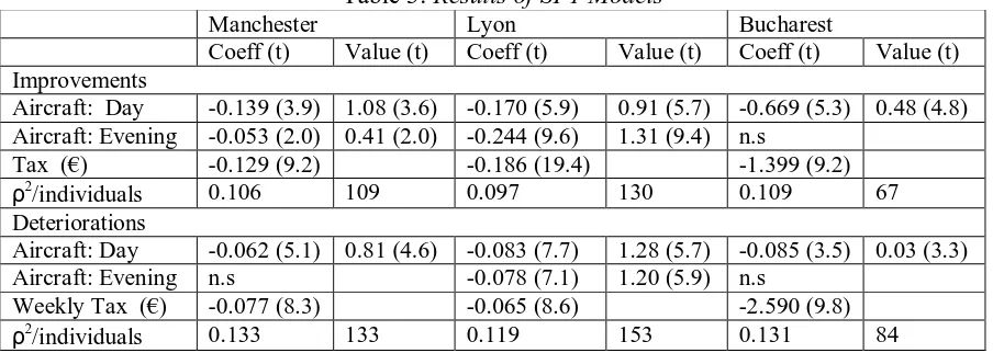
[image:7.595.221.373.78.158.2]

4.2 SP2 and SP3

Table 8 indicates the extent to which SP2 and SP3 provide similar values by time period. Given the SP2 models could not provide robust results for all periods, we have compared across periods for which coefficients are reported for SP2 in Table 4. For each set of results, Table 8 presents the proportions that each value in a period form of the sum of values across all relevant periods. There is an encouraging degree of similarity between the relative valuations by time period for SP2 and SP3 for Manchester, especially for the improvements in SP3. The same can be said for Lyon and Bucharest, although with some large differences between the figures for night.

The similarity of the SP2 and SP3 results allows us to conclude that respondents can distinguish between the aircraft annoyance of different time periods and indicates that it is reasonable to estimate values by time period without considering all time periods simultaneously.

Table 8: Variations by Time Periods in SP2 and SP3

SP Change Period Manchester Lyon Bucharest

2 Both Weekday 6am-9am - 18.2% 15.6%

2 Both Weekday 9am- 6pm 6.2% 8.6% 17.2%

2 Both Weekday 6pm-10pm 15.3% 23.5% 15.0%

2 Both Saturday 6am-9am - - 18.3%

2 Both Saturday 9am-6pm 16.2% 7.2% -

2 Both Saturday 6pm-10pm - 13.3% -

2 Both Sunday 19.4% 7.3% 16.1%

2 Both Night 42.9% 21.8% 17.8%

Imp Det Imp Det Imp Det

3 Imp Weekday 6-9am - - 5.8% 6.2% 11.2% 11.1%

3 Imp Weekday 9am-6pm 11.5% 8.5% 8.0% 3.8% 7.9% 11.1% 3 Imp Weekday 6-10pm 18.2% 13.5% 6.4% 5.0% 16.4% 11.1%

3 Imp Saturday 6-9am - - - - 19.6% 11.1%

3 Imp Saturday 9am-6pm 14.5% 8.7% 12.6% 6.1% - -

3 Imp Saturday 6-10pm - - 19.4% 7.5% - -

3 Imp Sunday 13.5% 7.3% 17.2% 9.5% 12.1% 14.8%

[image:7.595.68.528.479.738.2]

(8)

G

paper ID:013/p.8

5. CONCLUSIONS

We can hypothesise that SP1 provides lower values than SP2 since the incentive to bias responses is less because the purpose of the exercise is masked. This has been shown to be the case. Moreover, the SP1 results do seem to us to be reasonable.

Whilst we have concerns about the absolute money values obtained from SP2 and SP3, since the purpose of the study is clear, the relative values by time period seem generally plausible. Not only that, but there was a convincing degree of similarity between the two which is encouraging in terms of the validity of the relative values. It demonstrates that values disaggregated by time period can be obtained without having to consider all time periods simultaneously.

Whilst SP1 is the preferred method for valuing aircraft noise, it can only do this at an aggregate level, such as all day values or else limited disaggregations such as daytime and evening. The whole object of the exercise would be defeated if a wide range of time periods or different aircraft types were considered since the emphasis placed on aircraft movements would reveal the purpose of the study.

Thus the two approaches here have a complementary role. On the one hand, we believe that the quality of life exercise can provide reliable estimates of aircraft noise at an aggregate level but is unable to support disaggregations by time of day and aircraft type. On the other hand, we conclude that a conventional SP exercise provides inflated absolute values but that its contribution is in terms of providing relative valuations by time period or aircraft type which can be used to decompose overall values.

REFERENCES

[1] Hague Consulting Group (2000) ALOGIT 4.0EC. The Hague.