Essays on family, health Inequalities and labor dynamics

Texto completo

(1)Essays on Family, Health Inequalities and Labor Dynamics. Yuliya Kulikova. ADVERTIMENT. Lʼaccés als continguts dʼaquesta tesi queda condicionat a lʼacceptació de les condicions dʼús establertes per la següent llicència Creative Commons: http://cat.creativecommons.org/?page_id=184 ADVERTENCIA. El acceso a los contenidos de esta tesis queda condicionado a la aceptación de las condiciones de uso establecidas por la siguiente licencia Creative Commons: http://es.creativecommons.org/blog/licencias/ WARNING. The access to the contents of this doctoral thesis it is limited to the acceptance of the use conditions set by the following Creative Commons license: https://creativecommons.org/licenses/?lang=en.

(2) Universitat Autònoma de Barcelona Facultat de Ciències Econòmiques Departament d’Economia i d’Història Econòmica Doctorat en Anàlisi Econòmica. Doctoral Thesis. Essays on Family, Health Inequalities and Labor Dynamics. Author:. Supervisors:. Yuliya Kulikova. Dr. Nezih Guner. Dr. Ana Rute Cardoso. April 2016.

(3) 2.

(4) Acknowledgments. Every now and then in our life it is good to stop for a while and look backwards, evaluate what was has been achieved and build new plans for future. It looks like finishing this dissertation is one of such moments for me, a moment to make a brief pause, think about a several-years journey that is called "Graduate School" and especially thank all those people who made it possible, who were nearby during these very interesting, challenging but sometimes tough and stressful times. First and foremost, I would like to thank my best advisor ever, Nezih Guner. Nezih, I am an extremely lucky and happy person to be your student, truly, you cannot dream for a better teacher. I admire you not only because you are the great researcher with great ideas, but also you as a personality, curious about everything around us, easily breaking the borders between different fields and acquiring new interests, so caring about everyone around you, so supportive, patient and encouraging.. Every time when something was. going wrong with my research, I was entering your office broken, lost and hopeless, and I was leaving it engaged, optimistic and ready to move mountains. I can not thank you enough for everything you have done for me. Another person that affected me in so many positive ways and who helped me a lot throughout the PhD is Joan Llull, my coathor, who became a real friend. learned so much from you!. Joan, I’ve. You opened new fields for me and definitely shaped my. scientific interests. It felt so good working until late, on weekends or in summer, knowing that the next door there was someone else, who is working hard, setting high standards for himself. Thank you for your every day smile, willingness to talk even under the time pressure and you excitement about the world. There are many other professors in the IDEA and IAE that I would like to acknowledge. Ana Rute Cardoso – for your kindness and for giving a chance to finance my studies. Miguel Ángel Ballester – you spend an eternity explaining me the sequence spaces, thank you for believing in me and for your patience. Maite Cabeza, Michael Creel, Juan Enrique Martínez-Legaz – for a great teaching assistantship experience, I have learned a lot from you. Kiku Obiols – for your enormous optimism, constant jokes and support, your enthusiasm in discussions and a lot of feedback. Jordi Caballé, David Pérez-Castrillo, Inés Macho, Pedro Rey, Tomás Rodríguez-Barraquer, Johannes Gierlinger – your support and advice during the job market time was invaluable. Hannes Mueller and (again) Joan Llull – for beautiful passionate discussions in applied group. Javier Fernández Blanco, Sekyui Choi, Angela Fiedler, Joachim Jungherr – for profound discussions on the best macro papers and for understanding that even if you understand things there are a lot more things in them to understand. Special thanks to Evi Pappa – the fountain of creativity, in discussions with you I always felt energy and passion about research. Àngels, Mercè, you were always there to help. Without you all the bureaucracy issues would become just a nightmare. Thank you for eagerness to help and for your smiles. I would like to thank Gustavo Ventura for hosting me during my visiting period of. 3.

(5) Arizona State University. My time there was crucial for maturing as an professional. I acknowledge financial support from the Spanish Council for Scientific Research (CSIC) and from the Spanish Ministry of Economy and Competitiveness, through fellowship CSIC-JAE-PreDoc JAEPre002_2010_01226 and Grant ECO2013-49357-EXP. A lot of thanks to my very best colleagues and amazing officemates: Francesco, Isabel, Benjamin, Dilan, Alberto, Javi, Alex, Edgardo, John, Tugce, Guillem (Vasya), Rodica; to my "academic brothers and sisters" – Andrii, Matt, Alessandro, Lesha, Alejandra, Ezgi, Chris, Efi. It was a great pleasure to share this part of my life with you. Arnau and Dima, you are my specials, you were always the first ones to discuss ideas, news and problems, thanks for making this journey together. I was missing you so much during my job market year! My beloved friend Anechka, I am indebted to you, you put so much faith in me, that I always feel I cannot fail you, thanks for staying so close being so far. Gratitude to my dearest friends Tanechka, Katya, Natasha, Max, everyone else, who found time to come and visit – the time I spent with you walking around amazing Barcelona, balanced the pleasure of constant work with the pleasure of leisure activities. And a huge thank you goes to everyone in the Kondrashov’s lab, my Barcelona family: Margo, Inna, Natalia, Dima, Petya, Anyuta, Dinara, Julia, Karen, Katya, Masha, Vika. My dear family, Valentina, Alexander, and Anton, thank you for your unconditional support in every decision I make. You were always with me despite geographical distance and a big difference in time zones, at the times of downs when I mostly needed you, and in the times of ups just being happy for me. Habibik, my love, my inspiration, without you this journey would just not happen. Thank you for "the pleasure of finding things out", and thank you for your care and love. A new chapter is opening.. 4.

(6) Contents. Acknowledgments. 3. Introduction. 10. 1 Health Policies and Intergenerational Mobility. 13. 1. Introduction . . . . . . . . . . . . . . . . . . . . . . . . . . . . . . . . . . .. 2. Related Literature. . . . . . . . . . . . . . . . . . . . . . . . . . . . . . . .. 16. 3. The Model . . . . . . . . . . . . . . . . . . . . . . . . . . . . . . . . . . . .. 17. 3.1. Health, Ability and Human Capital . . . . . . . . . . . . . . . . . .. 18. 3.2. Government . . . . . . . . . . . . . . . . . . . . . . . . . . . . . . .. 20. 3.3. Household Problem . . . . . . . . . . . . . . . . . . . . . . . . . . .. 22. Estimation . . . . . . . . . . . . . . . . . . . . . . . . . . . . . . . . . . . .. 26. 4.1. First-step estimation. . . . . . . . . . . . . . . . . . . . . . . . . . .. 26. 4.2. Second-step estimation . . . . . . . . . . . . . . . . . . . . . . . . .. 33. 4.3. Role Of Health. 4. 5. 5.1 6. . . . . . . . . . . . . . . . . . . . . . . . . . . . . .. Counterfactual Policy Experiments. 41. . . . . . . . . . . . . . . . . . . . . . .. 42. . . . . . . . . . . . . . . . . . . . . . . . . . . . .. 46. . . . . . . . . . . . . . . . . . . . . . . . . . . . . . . . . . . .. 48. Future directions. Conclusions. 13. 2 Marriage and Health: Selection, Protection, and Assortative Mating. 49. 1. Introduction . . . . . . . . . . . . . . . . . . . . . . . . . . . . . . . . . . .. 2. Data and Descriptive Statistics. . . . . . . . . . . . . . . . . . . . . . . . .. 52. 3. Model Specification and Identification . . . . . . . . . . . . . . . . . . . . .. 56. 4. Estimation Results: the Marriage Health Gap. 5. 6. 4.1. Main Results. 4.2. Robustness. 49. . . . . . . . . . . . . . . . .. 59. . . . . . . . . . . . . . . . . . . . . . . . . . . . . . .. 59. . . . . . . . . . . . . . . . . . . . . . . . . . . . . . . .. 61. Exploring Selection and Protection Mechanisms. . . . . . . . . . . . . . . .. 63. 5.1. Self-Selection into Marriage and Divorce. . . . . . . . . . . . . . . .. 64. 5.2. Assortative Mating by Health. . . . . . . . . . . . . . . . . . . . . .. 68. 5.3. Healthy Behavior . . . . . . . . . . . . . . . . . . . . . . . . . . . .. 70. 5.4. Health Insurance. 74. 5.5. Health Accumulation Through Marriage. Conclusions. . . . . . . . . . . . . . . . . . . . . . . . . . . . . . . . . . . . . . . . . . . .. 74. . . . . . . . . . . . . . . . . . . . . . . . . . . . . . . . . . . .. 75. 3 Household Labor Market Dynamics. 77. 1. Introduction . . . . . . . . . . . . . . . . . . . . . . . . . . . . . . . . . . .. 77. 2. Data on Labor Market Stocks and Flows . . . . . . . . . . . . . . . . . . .. 78. 3. Labour Market Stocks. . . . . . . . . . . . . . . . . . . . . . . . . . . . . .. 80. Household Level Measures of Unemployment . . . . . . . . . . . . .. 83. 3.1. 5.

(7) 4. Labor Market Flows . . . . . . . . . . . . . . . . . . . . . . . . . . . . . . 4.1. Individual Transitions. 4.2. Joint Transitions. 4.3. A Decomposition Exercise. 84. . . . . . . . . . . . . . . . . . . . . . . . . .. 84. . . . . . . . . . . . . . . . . . . . . . . . . . . . .. 86. . . . . . . . . . . . . . . . . . . . . . . .. 90. 5. Added Worker Effect . . . . . . . . . . . . . . . . . . . . . . . . . . . . . . 101. 6. Conclusions. . . . . . . . . . . . . . . . . . . . . . . . . . . . . . . . . . . . 105. A Appendix to Chapter 1 A.1. 115. Children Ability Distribution. . . . . . . . . . . . . . . . . . . . . . . . . . 115. B Appendix to Chapter 2 B.1. 116. Data Description and Variable Definitions. . . . . . . . . . . . . . . . . . . 116. B.1.1. Sample Selection. B.1.2. Variable Definitions . . . . . . . . . . . . . . . . . . . . . . . . . . . 117. . . . . . . . . . . . . . . . . . . . . . . . . . . . . 116. B.2. Descriptive Statistics . . . . . . . . . . . . . . . . . . . . . . . . . . . . . . 119. B.3. Detailed Baseline Results . . . . . . . . . . . . . . . . . . . . . . . . . . . . 122. B.4. Self-Selection into Marriage and Divorce, and Assortative Mating: Additional Results. . . . . . . . . . . . . . . . . . . . . . . . . . . . . . . . . . . 123. C Appendix to Chapter 3. 125. 6.

(8) List of Tables. 1.1. Parental life cycle health profile. . . . . . . . . . . . . . . . . . . . . . . . .. 28. 1.2. Parental hours conditional on health. . . . . . . . . . . . . . . . . . . . . .. 28. 1.3. Children’s hours conditional on health in period 3 if no college. . . . . . . .. 29. 1.4. Productivity life-cycle. Married. . . . . . . . . . . . . . . . . . . . . . . . .. 29. 1.5. Productivity life-cycle. Singles . . . . . . . . . . . . . . . . . . . . . . . . .. 29. 1.6. Parental life cycle ability profile. Married . . . . . . . . . . . . . . . . . . .. 30. 1.7. Parental life cycle ability profile. Singles. . . . . . . . . . . . . . . . . . . .. 31. 1.8. Marital and child-bear shocks. . . . . . . . . . . . . . . . . . . . . . . . . .. 31. 1.9. Children’s productivity in period 3 if no college. . . . . . . . . . . . . . . .. 32. 1.10 Estimates for insurance function . . . . . . . . . . . . . . . . . . . . . . . .. 33. 1.11 Ability transitions conditional on health and educational spending . . . . .. 35. 1.12 Estimated Parameters. 37. . . . . . . . . . . . . . . . . . . . . . . . . . . . . .. 1.13 Health production function. Baseline probabilities and marginal effects. . .. 1.14 Ability production function. Baseline probabilities and marginal effects. 38. . .. 38. . . . . . . . . . . . . . . . . . . . . . . . . . . . . . . . . . . . .. 40. 1.16 Role of Health . . . . . . . . . . . . . . . . . . . . . . . . . . . . . . . . . .. 41. 1.17 Counterfactual Experiments: Early and Late Education . . . . . . . . . . .. 42. 1.15 Model Fit. 1.18 Counterfactual Experiments: Early and Late Education Policies, by Parental Income Quintile . . . . . . . . . . . . . . . . . . . . . . . . . . . . . . . . . 1.19 Counterfactual experiments: Medicaid. 43. . . . . . . . . . . . . . . . . . . . .. 44. 1.20 Counterfactual experiments: Medicaid, by Parental Income Quintile . . . .. 45. 1.21 Counterfactual experiments: joint effect of educational and health policies .. 46. 1.22 Counterfactual Experiments: Joint Effect of Educational and Health Policies, by Parental Income Quintile. . . . . . . . . . . . . . . . . . . . . . . .. 47. 2.1. Marriage Ratios and Transitions In and Out of Marriage by Age . . . . . .. 54. 2.2. Correlation between Innate Health and Observable Characteristics . . . . .. 65. 2.3. Empirical Distribution of Innate Health . . . . . . . . . . . . . . . . . . . .. 66. 2.4. Health and Marriage/Divorce Probabilities . . . . . . . . . . . . . . . . . .. 67. 2.5. Contingency Tables: Assortative Mating by Innate Health. . . . . . . . . .. 69. 2.6. Correlation of Husband’s and Wife’s Innate Permanent Health . . . . . . .. 70. 2.7. Probability of Quitting Smoking and Marital Transitions. . . . . . . . . . .. 73. 3.1. Joint average labor market transitions of married couples . . . . . . . . . .. 86. 3.2. Conditional average labor market transitions for married couples . . . . . .. 90. 3.3. Explained variation (in %) of joint labor market stocks by the two most important transitions.. 3.4. . . . . . . . . . . . . . . . . . . . . . . . . . . . . .. 96. Explained variation (in %) of employment, unemployment, and participation by the two most important transitions.. 7. . . . . . . . . . . . . . . . . .. 97.

(9) 3.5. Counterfactual participation rate, employment and unemployment . . . . . 103. 3.6. Counterfactual participation rate, employment and unemployment during recessions and normal times. 3.7. . . . . . . . . . . . . . . . . . . . . . . . . . . 104. Contribution of the added worker effect to the household unemployment measures . . . . . . . . . . . . . . . . . . . . . . . . . . . . . . . . . . . . . 104. B.1. Descriptive Statistics: Panel Study of Income Dynamics (PSID). B.2. Descriptive Statistics: Medical Expenditure Panel Survey (MEPS) . . . . . 120. B.3. Estimated Coefficients from Baseline Regressions. B.4. Health and Marriage/Divorce Probabilities: Additional results. B.5. Contingency Tables: Assortative Mating from Chronic Conditions . . . . . 124. 8. . . . . . . 119. . . . . . . . . . . . . . . 122 . . . . . . . 123.

(10) List of Figures. 2.1. Health and Marital Status (PSID and MEPS). . . . . . . . . . . . . . . . .. 54. 2.2. Health and Marital Status for Different Socioeconomic Groups . . . . . . .. 55. 2.3. Unobserved Heterogeneity and the Self-Selection Bias: An Example. . . . .. 57. 2.4. Marriage Health Gap: OLS and Fixed-Effects Estimation Results. . . . . .. 60. 2.5. Marriage Health Gap: Grouped Fixed-Effects Estimation Results. . . . . .. 61. 2.6. Marriage Health Gap: System-GMM Estimation Results. . . . . . . . . . .. 62. 2.7. Alternative Health Measures . . . . . . . . . . . . . . . . . . . . . . . . . .. 63. 2.8. Alternative Definitions of Married and Single . . . . . . . . . . . . . . . . .. 64. 2.9. Preventive Health Checks and Marital Status. 71. . . . . . . . . . . . . . . . .. 2.10 Median Health Expenditures and Marital Status . . . . . . . . . . . . . . .. 72. 2.11 Health Insurance, Health, and Marital Status. . . . . . . . . . . . . . . . .. 75. . . . . . . . . . . . . . . . . . . .. 76. 2.12 Health Accumulation Through Marriage 3.1. Joint labor market stocks for married couples.. 3.2. Joint labor market stocks for married couples by educational categories. . .. 82. 3.3. Individual Unemployment Rates of Males and Females. 83. 3.4. Unemployment Measures and their Cyclical Components. 3.5. Unconditional labor market transitions of males and females. 3.6. Labor market transitions for married males conditional on spouse’s state tomorrow. 3.7. . . . . . . . . . . . . . . . . . . . . . . . . . . . . . . . . . . . . . . . . . . . . .. . . . . . . . . . . . . . . . . . . . . . . . . . . . . . . . . . . . .. 81. 84 85 88. Labor market transitions for married females conditional on spouse’s state . . . . . . . . . . . . . . . . . . . . . . . . . . . . . . . . . . . .. 89. 3.8. tomorrow. Decomposition exercise for joint labor market states . . . . . . . . . . . . .. 92. 3.9. Decomposition of employment rates: everyone, males and females. . . . . .. 98. 3.10 Decomposition of unemployment rates: everyone, males and females . . . .. 99. 3.11 Decomposition of participation rates: everyone, males and females . . . . . 100 3.12 Added Worker Effect and Participation rate, Employment and Unemployment . . . . . . . . . . . . . . . . . . . . . . . . . . . . . . . . . . . . . . . 102 3.13 Added Worker Effect and the Data. . . . . . . . . . . . . . . . . . . . . . . 105. A.1. Ability distribution for different age groups . . . . . . . . . . . . . . . . . . 115. B.1. Health and Marital Status, Different Socioeconomic Groups (MEPS). C.1. Important joint labor market transitions. 9. . . . 121. . . . . . . . . . . . . . . . . . . . 125.

(11) Introduction. It’s hard to overestimate the role of family in our lives. Starting from the initial endowments that we get from our parents through genes, continuing with parental investments into our education, health, personality, to the choices that we make ourselves for creation of our own families: giving birth to children, passing them our genes and participating in their life in so many ways.. As an economist, I am extremely interested in the way. families affect socioeconomic outcomes, such as health, education, labor supply, and income. This thesis consists of three chapters in which I consider family as a basic unit of the decision-making in the economy and I study the implications of these decisions for health inequalities and labor supply, very important socioeconomic outcomes. In the first chapter of this thesis I study the role of health, health policies, and parental investments into their children, for transmission of income over generations within the same family. In the second chapter I look at family dynamics itself and investigate what is the role of marital status for health inequalities in the society. In the last chapter, I study how decisions at the family level may affect labor market dynamics. In the first chapter of this thesis, named. bility",. "Health Policies and Intergenerational Mo-. I study the role of health inequalities and health policies for income persistence. over generations within family in the United States. According to recent estimates (Solon, 2002; Mazumder, 2005), the intergenerational correlation of income in the U.S. is high, around 0.4 to 0.6. This results in very different opportunities for children from rich and poor families. So, children of the families in the upper income quintile have 32% probability of staying in the upper income quintile, while only 9% of children from the families in bottom income quintile will reach the top income quintile during their lifetime. What is the importance of health and health policies for social mobility and inequality in the U.S.?. While the role of education and education policies received a lot of attention in. the literature on intergenerational mobility, we know very little about the role of health policies.. This is rather surprising since, like education, health is persistent across gen-. erations, and affects an individual’s lifetime income both directly (through limiting his capabilities) and indirectly (through its effect on human capital accumulation).. This. chapter is devoted to investigation of the importance of health and health policies for intergenerational income persistence and income inequality.. I develop and estimate an. overlapping generations model populated by heterogeneous households. I distinguish two forms of human capital: human capital, that is an innate ability enhanced by education, and health capital, which affects human capital accumulation during childhood and an individual’s capabilities (how much he can exploit his human capital) as an adult. Hence, in the model households differ by health and human capital of parents and children. They also differ, however, by their family structure (single parents versus married couples) and fertility status (some households are childless while others have children in different points in their life-cycle). The model takes into account multidimensionality and dynamic and self-productive nature of human capital investments (as in Cunha, Heckman and Schen-. 10.

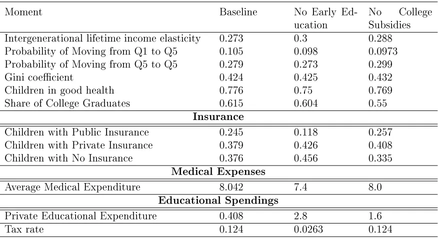
(12) nach (2010)). When deciding on investments into their children’s health and education, parents take into account government policies on health and education. Government provides subsidies for early and late (college) education. It also runs a means-tested medical insurance program which is modeled to capture the key features of the Medicaid program in the U.S. Besides means-tested public insurance, the households also have access to private health insurance. I bring this structural model to the data and replicate important data moments for the U.S., related to insurance market, education, and health; and then I perform several counterfactual experiments with medical and educational policies.. I. find that both medical and education policies affect intergenerational mobility in the U.S. significantly, although the scale of the effect on average is moderate. There are important interactions between health and education policies. Changes in both policies have a larger effect than each one in isolation. Especially this interaction effect is important for children of the lowest income quintile. When Medicaid is eliminated, parents face a trade-off between spending their resources on education versus on health of their children. However, if we eliminate both educational policies together with the Medicaid policy, this trade-off becomes much more significant, especially for poorer households. As a result, we observe a huge increase in parental decisions gap regarding their investments in health and education of their children.. If richer parents have resources to substitute for lost. governmental investments into health and education of their children, poor households are constrained. They try hard to substitute for lost health policies but they give up on investments into education as health and ability are complements, and investments into education become inefficient for them. For rich parents the decisions look very different, they sacrifice slightly with their investments into health which results in slightly lower health levels for children, however they increase a lot investments into education to ensure high human capital for their children by the time of entering labor market. Thus, the gap in health between children from rich and poor households persists, the gap in ability between rich and poor children increases a lot, which results in higher income persistence and lower mobility in general. In the second chapter of this thesis. Assortative Mating". "Marriage and Health: Selection, Protection, and. (joint with Nezih Guner and Joan Llull), we study how marital sta-. tus affects health inequality. Married people are healthier than non-married people along the entire life cycle, with the difference of 3% in self-reported health for younger individuals and up to 12% at ages 50-60 years. There are two ways to interpret these results. First, marriage could have a protective effect, with marriage helping to ensure healthier food, more exercise or a reduction in risky behavior.. Second, the difference could be. attributed to selection into marriage whereby healthier people have higher probability to marry and stay married. We used panel data techniques, such as within-group estimation, grouped fixed effect estimation (like in Bonhomme and Manresa (2015)) and system generalized method of moments estimation (like in Arellano and Bover (1995)) to control for unobserved heterogeneity. We find that both selection and protective effects of marriage contribute to the difference at large, however, selection explains all of the effect for younger individuals, with a 6% protective effect of marriage for middle aged couples. We find that the benefits of marriage on health are cumulative, with 10 extra years of marriage increasing the probability of being healthy by about 3 percentage points remaining roughly constant after 35-39. We then explored possible mechanisms of marriage protection effects. Our results show that there are significant differences between married and single individuals for all categories of preventive care, access to health insurance, healthy behavior and medical expenditures. Thus, even though the selection effect into marriage. 11.

(13) is rather large, marital status appears one of the determinants of health inequality over the life cycle. In the third chapter of this thesis,. "Household Labor Market Dynamics", coauthored. with Nezih Guner and Arnau Valladares-Esteban, we study the role of labor supply decisions within family for the labor market dynamics. Why do we think it is important to look at households rather than individuals? On the one hand, family provides insurance from negative labor market shocks. As a result, an unemployed married person can rely on his partner’s income while looking for a suitable job.. On the other hand, having a. partner may constrain job market options for dual career concerns (Guler, Guvenen and Violante, 2012; Browning, Chiappori and Weiss, 2014). Understanding the link between families and labor market outcomes, such as unemployment, may be important not only for explaining the evolution of unemployment, but also for labor market policies. In this chapter we study the joint labor market transitions of married couples between three labor market states: employment, unemployment, and out of the labor force. The results show that joint labor market transitions are important to understand both the secular rise in aggregate employment and the cyclical movements in unemployment. Following a decomposition exercise proposed by Shimer (2012), we assess the importance of different labor market transitions for married males and females.. The results show that married men. and women differ in their labor market dynamics. The transition between employment and unemployment is the key driver of cyclical movements in unemployment for married males. For married females, however, transitions in and out of the labor force play a key role. Hence modeling out of labor force as a distinct state is critical to understand joint labor market dynamics of married couples. The results also show that joint labor market transition of husbands and wives is affected by the coordination between labor market activities of household members. In particular, we concentrate on analysis of the "added worker effect", one of the ways spouses coordinate that results in an increase in married women’s labor supply in response to their partner’s unemployment spells. Previous literature, e.g. Lundberg (1985), Stephens (2002) and Juhn and Potter (2007) show that women’s labor supply is quite responsive to their partner’s entry into unemployment. We find that without the added worker effect, female labor participation and unemployment rates in 2000-2010 period would be about 2.5 and 0.3 percentage points higher, respectively. This 0.3 percentage points represents about 6.16% of the female unemployment rate. On the other hand, the added worker effect lowers the fraction of households with no employed members by about 0.4 percentage points in the same period, which is a significant (about 13.3%) of the fraction of households with no employed members.. 12.

(14) Chapter 1 Health Policies and Intergenerational Mobility. 1. Introduction. Parental characteristics, such as education, earnings, income, and health are strongly correlated with the same outcomes for children. Estimates of intergenerational elasticity of income, a common measure of intergenerational mobility, varies around 0.4-0.6 for the. 1. US – Solon (2002), Solon (2004), Zimmerman (1992), and Mazumder (2005).. These. estimates imply that if a parent is 10% richer than the average person in the economy, his. 2. sun is likely to be 4-6% richer as well.. Intergenerational elasticity of life span of parents. and children in the US is 0.28, and it is higher for father-son (0.356) and mother-daughter (0.32) pairs – Parman (2012). Furthermore, intergenerational mobility is closely related with inequality in a society. In societies with higher income inequality social mobility is lower, especially at the tails of the income distribution.. This relation is called "Great. Gatsby Curve", see Corak (2013), and it makes the "lottery" in which family a child is born in even more important – Chetty, Hendren, Kline and Saez (2014). Recent literature shows that initial (pre-labor market conditions) are very important in determining later labor market outcomes of children. For example, Keane and Wolpin (1997) find that unobserved heterogeneity at age 16, explains about 90% of variation in lifetime utility.. Huggett, Ventura and Yaron (2011) find that differences in initial. conditions (human capital and wealth) at age 23 are more important than shocks received over the working lifetime for the variation in lifetime earnings, lifetime wealth, and lifetime utility. The key question is of course what determines initial conditions of children. First, genes, or as it is labeled in the literature, nature matters: parents with better health/ability are more likely to give birth to more healthy/able children. Second, nurture, the environment in which children grow, plays an important role.. Family background,. such as education, parental abilities, health, and earnings determines the environment in which a child is growing up.. If parents are educated, healthy and rich, the child most. 1 Corak (2013) and Guner (2015) review the recent literature on intergenerational mobility. 2 Intergenerational income elasticity is calculated by regressing the log earnings of sons on log earnings of fathers, controlling for ages of both.. However, there are other ways of estimating degree of inter-. generational mobility. For example, Chetty et al. (2014) use correlation of parent’s and child’s income percentile ranks or calculate transition probability of moving from the bottom quintile to the upper one, while Güell, Mora and Telmer (2015) and Clark (2014) use joint distribution of surnames and economic outcomes to study intergenerational mobility.. 13.

(15) probably will also be educated, healthy and rich.. But what if parents are poor, not. educated or not healthy? Their children are disadvantaged comparing to the children of healthy, educated and rich parents.. The government policies then can play a role and. try to equalize opportunities for all children, independently of their family background. Providing access to education and to health facilities, government may counteract the role of parental earnings and disadvantaged environment at home. Education is known to be an excellent social lift (Restuccia and Urrutia (2004), Caucutt and Lochner (2012), Lee and Seshadri (2014)). On the other hand, we know almost nothing about how medical policies affect intergenerational mobility and inequality. To the best of my knowledge there are only few empirical papers devoted to this question. Mayer and Lopoo (2008) analyze association of total government spending and intergenerational mobility, using variation in the amount of government spending in different US states.. They find that higher government spending reduce the importance of parental. income for the economic success of children. Furthermore, Aizer (2014) analyzes empirically the relation between intergenerational mobility and different welfare policies, such as foster care, family planning, income transfer programs, residential mobility interventions, educational interventions and public health.. Among all welfare policies she considers,. increases in spending on health are most strongly associated with reductions in the importance of family background and declines in inequality in the production of child human capital (measured as PISA test scores among 15 year-olds). Case, Lubotsky and Paxton (2002) study health-income gradient, i.e. that children born to low-income parents tend to be in worse health status than children born to high-income parents. They find that neither health at birth, nor access to health insurance affects estimates of health-income gradient, and conclude that health affects intergenerational mobility through other channels, such as parental investments into health. Finally, O’Brien and Robertson (2015), study how Medicaid expansion of 1980s and 1990s affected intergenerational mobility using geographical variation in policy changes and find a positive, but not very large, effect of Medicaid on mobility. They find that increasing the proportion of women aged 15-44 eligible for Medicaid is associated with reduction in rank correlation of incomes of parents and children. They also find that children born to low-income parents after Medicaid expansions are more likely to move upwards. Brown, Kowalski and Lurie (2015) also show that Medicaid expansion affected child’s income significantly positively, however they were not studying implications of this for intergenerational mobility. Cohodes, Kleiner, Lovenheim and Grossman (2014) explore the same Medicaid expansion of 1980s and 1990s and find that it had a substantial positive effect on child’s schooling outcomes. Hence, while there is some evidence that suggests that health is important for intergenerational mobility, there has not been any attempts to understand the mechanisms through which health and health policies affect intergenerational mobility. Meanwhile the U.S. government spends significant amount of resources on needs-based medical policies. In June 2013, over 28 million children were enrolled in Medicaid and another 5.7 million were enrolled in State Child Health Insurance Program (SCHIP).. 3. 4. Yet, according to 2012 National Health Interview Survey , 36% of families with children in the United States experienced financial burden of medical care, such as problem paying medical bills in the past 12 months, having currently medical bills that they are unable to pay, having currently medical bills that are being paid over time. Poorer families are. 3 Source:. http://kff.org/health-reform/issue-brief/childrens-health-coverage-medicaid-chip-and-the-aca/ 4 Source: http://www.cdc.gov/nchs/data/databriefs/db142.htm. 14.

(16) more likely to experience burden of medical care than the richer ones.. In particular,. families with income between 139% and 250% of Federal Poverty line (FPL) are affected the most, and this is exactly the group that is not always covered by Medicaid and SCHIP. On the other hand, government policies can also crowd out family investments (Cutler and Gruber 1996). How do then parents allocate their limited recourses between medical expenses and expenditures on other forms of human capital, such as education? Is poor health of children a barrier for upward mobility? How do a large-scale policy intervention, like Medicaid, affect intergenerational mobility and inequality? How do policies on health and education interact? These are the questions I try to answer in this thesis chapter. I develop a human-capital based overlapping generations model of household decisions that take into account multidimensionality and dynamic nature of human capital investments. Following Grossman (1972), I model health as a human capital and hence distinguish two forms of human capital: health capital and human capital (ability). I assume that human capital eventually determines person’s productivity while health capital determines physical capacity of acquiring and enjoying productivity. I follow Cunha, Heckman and Schennach (2010) and allow for dynamic complementarity and self-productivity. 5. of human capital.. These two factors produce a multiplier effect since one type of human. capital enhances production of the other type of human capital. Parents decide on consumption and investments into human and health capital of their children. These investment decisions, together with intrinsic health and ability that is correlated across generations, determine future health and productivity of children when they become adults.. Health and human capital of adults define their physical. ability to work and labor market productivity. I model explicitly governmental policies in education and health.. Government provides educational spending on primary and. secondary education, as well as income-based subsidies for college education. Furthermore, it provides income-based medical policy that closely mimics Medicaid in the U.S. In this chapter I replicate important data moments for the US and then I perform several counterfactual experiments with medical policies. Results show that Medicaid as well as both education policies (early and late) affects intergenerational mobility in the US. There are important interactions between health and education policies. Changes in both policies have a larger effect than each one in isolation. Especially this interaction effect is important for children of the lowest income quintile.. When Medicaid is eliminated,. parents face a trade-off between spending their resources on education versus on health of their children. When both college subsidies and Medicaid are eliminated, this tradeoff becomes much more significant, especially for poorer households.. As a result, we. observe that poor households do not invest into early education at all (and also they don’t go to college in absence of college subsidies), while richer households substitute health investments (and as a result lower health level) by higher educational spending (and as a result higher ability). The remainder of the chapter is organized as follows: in section 2 I provide a short literature review, section 3 is devoted to the model description, section 4 presents model estimation strategy and benchmark model, in section 5 on can find results for the counterfactual experiments, section 6 concludes.. 5 Self-productivity means that human capital produced at one stage make further human capital production more efficient.. Dynamic complementarity means that levels of human capital investments at. different ages are synergistic and fortify each other.. 15.

(17) 2. Related Literature. This work is naturally related to the large literature on intergenerational mobility and inequality. This literature dates back to Becker and Tomes (1979, 1986) and Loury (1981), who explore implications for intergenerational mobility of credit constraints and ability persistence over generations. Following their seminal contributions, a large body of literature is devoted to understand sources of intergenerational mobility and inequality as well as how different public policies affect them. First, it is well known that inequality and social mobility are negatively correlated (Corak, 2013). However, policies that mitigate inequality do not necessarily work well to increase intergenerational mobility (Becker, Kominers, Murphy and Spenkuch, 2015). Second, recent literature shows that parental investments into human capital (education) is a very important channel for intergenerational correlation of incomes. Becker et al. (2015) in their theory of intergenerational mobility find that even in a world of perfect capital markets with no differences in ability rich parents tend to invest more into their children’s human capital than poor parents and as a result in the top of distribution earnings persistence is stronger than in the middle. There is a very large literature that shows that early childhood investments are very important in determining human capital of a child when he becomes adult (Cunha and Heckman, 2007; Cunha, Heckman and Schennach, 2010; Heckman, Yi and Zhang, 2013). Family environment along with family in vestments play a crucial role in this process (Carneiro and Heckman, 2003; Cunha, Heckman, Lochner and Masterov, 2006).. Lefgren, Lindquist and Sims (2012) examine. two transmission channels for intergenerational persistence of income:. causal effect of. parental income and causal effect of parental human capital. They find that both channels are active, around 37% is due to the causal impact of father’s financial resources, the remainder is due to the transmission of father’s human capital. Restuccia and Urrutia (2004) build an overlapping generations model with early and late investment in human capital. Their simulations show that around half of intergenerational correlation in earnings is attributed to parental investments into education (particularly, early education). Building a similar model, Caucutt and Lochner (2012) suggest that financial constraints might prevent parents from effective investments into their children. And as a result differences in initial conditions by the age of 20-25 explain up to 60% of variation in lifetime earnings, according to Huggett et al. (2011). Third, government can intervene and affect both, intergenerational mobility and inequality. Lee and Seshadri (2014) also build an overlapping generations model with early and late investment in children human capital. They also allow on-the-job human capital investments for adults. They find that education subsidies and progressive taxation can significantly reduce the persistence in economic status across generations.. However, it. should be kept in mind that government investments can crowd out family investments, that’s why it is important to keep in mind family responses to changes in government policies (Cutler and Gruber, 1996). Finally, institutional differences matter. Herrington (2015) compares the US and Norway in mobility and inequality and finds that tax system and public education spendings are responsible for about one-third of difference in inequality and 14% difference in intergenerational earning persistence between Norway and the US. Mayer and Lopoo (2008) assess the relationship between government spending and intergenerational economic mobility using PSID data and find greater intergenerational mobility in high-spending states compared to low-spending states. They also find that the difference in mobility between. 16.

(18) advantaged and disadvantaged children is smaller in high-spending states and that expenditures aimed at low-income populations increase the future income of low-income children but not high-income children. Rauh (2015) looks at importance of political economy for distributional effects in education and it’s implications for inequality and social mobility and finds that voter turnover can explain around one-fourth of cross-country differences in inequality and mobility. All of the papers mentioned above as well as others in the literature abstract from health, and human capital is simply modeled as a function of parental and public investment on education. The only exception is Heckman et al. (2013) who also consider health as one of the dimensions of human capital. They show that early health shocks negatively affect all dimensions of child human capital: health, education, socioemotional skills and this effect is very important for policy implications. On the other hand, the literature on health comes to a conclusion that health is very important in determining later life outcomes. Currie and Gruber (1996a,b) study the effects of the Medicaid expansion to pregnant women and low-income children and find big positive effect for children’s health and negative effect for child mortality. Prados (2013) quantifies the health-income feedback and states that it accounts for 17% of earnings inequality. In seminal Grossman (1972)’s paper the notion of health capital is introduced and health is modeled as a result of investments into health and it’s depreciation over time. This gave rise to macroeconomic models that incorporate health risks in a life-cycle framework. Attanasio, Kitao and Violante (2010), for example, study tax implications due to projected rise in medical spending financed through Medicare – governmentally provided partial insurance against negative health shocks for older people. Palumbo (1999) and De Nardi, French and Jones (2010a) study saving decisions of the elderly and the role of medical shocks in savings behaviour, Jung and Tran (2014) study medical expenditure behavior over the life cycle, separating pure age effects and cohort effects. Ozkan (2013) studies differences in the lifetime profile of health care usage between low- and high-income groups and finds that policies encouraging the use of health care (especially preventive) by the poor early in life have significant welfare gains, even when fully accounting for the increase in taxes required to pay for them. Kopecky and Koreshkova (2014) evaluate joint effect of social security and Medicaid on labor supply, savings, economic inequality and welfare due to idiosyncratic risks in labor earnings, health expenses and survival. Brown et al. (2015) study long-term impact of expansion of Medicaid and State Children’s Health Insurance Program that occurred in 1980’s and 1990’s and find that the government will recoup 56 percent of spending on childhood Medicaid by the time these children reach 60. However, papers on health and health policies typically ignore human capital dimension. The current work builds a bridge between literature on health and health policies on the one hand and human capital and human capital policies literature on the other and provides a more structural model to look at the relationship of health and health policies, their interaction with educational policies and intergenerational mobility.. 3. The Model Consider the following overlapping generations model. Time is discrete and the horizon is infinite. Each household consists of one child and parents. Parents can be single mothers or married couples (who act as a single decision making unit). Marital status of parents is denoted by. 𝜃=0. (single) and. 𝜃=1. (married). Each model period corresponds to 7. years. Each person lives for 8 periods: 3 as a child (0-7, 8-14, 15-21), denoted by. 17. 𝑗,. 5 as.

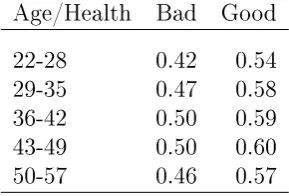
(19) adult (22-28, 29-35, 36-42, 43-49, 50-57), denoted by. 𝑡.. Fertility is exogenous; when a person becomes an adult, after 3 periods of childhood, she can have no child or one child that is born in the 1st (22-28), 2nd (29-35) or 3rd (36-42) period of the adulthood. The childbearing status is denoted by. 𝑏=1. (early childbearers),. 𝑏=2. (middle-age childbearers), and. 𝑏=3. 𝑏=0. (childless),. (late childbearers).. Besides marital status and fertility, households differ by human capital of parents and children. I allow for multidimensionality of human capital. Each child has bidimensional human capital: health capital (ℎ) and other types of human capital (𝑎). The latter includes cognitive and socioemotional skills. Similarly, each parent has her health capital. (𝐻) and human capital 𝐴 (whenever possible I use capital letters to indicate parental variables). Human capital determines earnings potential of an adult, while health determines how much labor he can supply. If a family does not have children, it just consumes everything.. If there is a child,. households make two sets of decisions. First, they decide whether or not to buy medical insurance for their children. Then, they decide how much to spend on his education and health. There is also a government in the economy that provides health insurance for poor households. The government also gives education subsidies. While the education subsidies are universal for early education, they are income based for late (college) education. * * Children are born with innate health (𝑎 ) and innate ability (ℎ ), which are correlated across generations. Innate ability, together with investment by parents, government policies and luck, transforms into future ability of a child and eventually determines his productivity as an adult. Similarly, innate health, together with health spending by parents, government policies and luck, transforms into future health of a child and eventually into his health status as an adult. Parents make decisions to maximize their lifetime utility and are altruistic, i.e. they care about their offspring’s utility when they become adults.. Thus, they care about. leaving their children with high levels of health and human capital. I abstract from assets and physical capital in the model. There is no aggregate uncertainty as well.. 3.1. Health, Ability and Human Capital Human capital is bidimentional, it consists of health capital and human capital.. I use. the term human capital and ability interchangeably. Ability determines an adult agent’s earnings potential. Health capital, on the other hand, determines the quantity of labor supplied by an adult individual on the labor market. health are inputs for the production of future ability.. For children, current ability and After three periods with their. parents, children become adults and their human capital and health capital determines their ability (productivity) and health as adults. A central feature of the model is health and human capital production.. Following. Cunha, Heckman and Schennach (2010) I allow for dynamic complementarity and self* productivity of human capital. Children start their life with innate health ℎ and innate * ability, 𝑎 , randomly drawn and correlated with their parent’s innate health and ability.. Γ𝑎* |𝐴* and Γℎ* |𝐻 * represent the Markov processes for innate ability and health, where 𝐴 and 𝐻 * are innate ability and health of parents. * Given ℎ1 = ℎ , during the childhood, next period’s health depends on previous period’s health, medical spending by parents, denoted by 𝑚, and a health shock, denoted by 𝜐 . In particular, I assume that health status takes two values, good or bad, and the probability that next period health is equal to ℎ𝑘 , 𝑘 ∈ {𝑔𝑜𝑜𝑑, 𝑏𝑎𝑑}, is given by the Let *. 18.

(20) following. logit relation. 𝑃 𝑟(ℎ′ = ℎ𝑘 |ℎ, 𝑚) = Λ(𝛼0ℎ + 𝛼1ℎ ℎ + 𝛼2ℎ 𝑚 + 𝛼3ℎ ℎ · 𝑚), (1.1) It is assumed that 𝜐 is independent and identically 𝜎𝜐2 . I allow these production functions be different in the early childhood (period 1 and 2) and late childhood (period 3).. where. Λ. is the logistic function.. distributed with zero mean and variance. After 3 periods of childhood, children become adults and health in the first period of adulthood is given by. ℎ ℎ ℎ ℎ ℎ · 𝑚). 𝑚 + 𝛼33 ℎ + 𝛼32 + 𝛼31 𝑃 𝑟(𝐻1 = 𝐻𝑘 |ℎ, 𝑚) = Λ(𝛼30 (1.2) Once. 𝐻1. is determined, future health as an adult is given by an exogenous process. which captures life-cycle health transitions. hours an adult can work, denoted by. 𝑄𝐻 ′ |𝐻 ,. Adult’s health determines the number of. 𝑇𝑡 (𝐻).. It is assumed that the effect of health on. hours work depends on the age of the parent. Every period parents and government invest into child’s ability. These investments, together with the current health and ability, determines next period’s ability. The process is, however, not deterministic and each period there is a shock for ability accumulation, denoted by 𝜀. It is independent and identically distributed with zero mean and variance 𝜎𝜀2 . In the 1st and 2nd periods, government provides each household with 𝑔 units of resources to invest on their children. Given educational spending, denoted by. 𝑒 ≥ 𝑔.. 𝑔,. parents can complement them with private. Ability production function in the 1st and 2nd. childhood periods take as inputs previous ability and health, amount of parental spending into education, as well as the random shock,. 𝜀𝑗 .. As health, human capital also can take. two values, low and high, and the probability that next period’s ability is equal to. 𝑘 ∈ {ℎ𝑖𝑔ℎ, 𝑙𝑜𝑤}. 𝑎𝑘 ,. is given by a logit function:. 𝑃 𝑟(𝑎′ = 𝑎𝑘 |𝑎, ℎ, 𝑒, 𝐴) = Λ(𝛼0𝑎 + 𝛼1𝑎 𝑎 + 𝛼2𝑎 ℎ + 𝛼3𝑎 𝑒+ 𝛼4𝑎 · 𝑎 · 𝑒 + 𝛼5𝑎 · ℎ · 𝑎 + 𝛼6𝑎 𝐴 + 𝛼7𝑎 𝐴 · 𝑒) (1.3) In the 3rd period of childhood, parents make a decision whether or not to send their child into college.. The college tuition is denoted by. parents qualify for subsidies to cover this tuition.. 𝐸.. Depending on their income,. If they don’t send their children to. college, children participate in the labor market during the last period of their childhood. Children then supply. 𝑡3 (ℎ3 ). hours in the market and contribute to household income.. After three periods of childhood, accumulated ability, health, along with decision on college education, determines the productivity of the child as an adult,. 𝐴1 .. The process 2 is also subject to a shock 𝜀3 , normally distributed with zero mean and variance 𝜎𝑖𝑛𝑐 , which captures the fact that within a cohort, earnings vary and more than one-third of the variance is attributable to post-education factors (Huggett et al., 2011). determined in the following way. First, for each child the following value. Π. 𝐴1. is. is calculated:. 𝑎 𝑎 𝑎 𝑎 𝑎 𝑎 𝑎 𝑐𝑜𝑙 + 𝛼34 · 𝑎 · ℎ + 𝛼35 · ℎ · 𝑐𝑜𝑙 + 𝛼36 · 𝑎 · 𝑐𝑜𝑙 + 𝜀3 . Π = 𝛼30 + 𝛼31 𝑎 + 𝛼32 ℎ + 𝛼33 (1.4). 19.

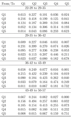
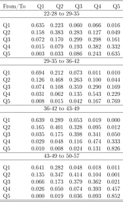
(21) Then four threshold income levels. 𝑥1 , 𝑥2 , 𝑥3 ,. 𝑥4. and. are selected such that about 20% of. children are in the first, second, third, fourth and fifth quintiles of a normal distribution 2 with zero mean and variance 𝜎𝑖𝑛𝑐 , and each child is placed into the corresponding income quintile as an adult. Starting from the first adult period, ability,. 𝐴1 ,. is characterized by the productivity 𝜃 quintile of an adult and is subject to an exogenous stochastic process, 𝑄𝐴′ |𝐴 that captures life-cycle behavior of productivity and is specific to the marital status 𝜃 .. 3.2. Government 𝜏. Government taxes income at a proportional tax. and spends tax revenue on education. and health. Governmental budget is balanced:. 𝜏 𝑌 = 𝐺 + 𝐹 + 𝑆, where. 𝑌. is the total income in the economy,. secondary education,. 𝐹. 𝐺. is the total spending on primary and. is the total spending on college subsidies, and. 𝑆. is the total. spending on Medicaid/SCHIP.. Education Policy. In the US, primary and secondary education is obligatory and is. guaranteed for all children of the age 5 to 18.. 6. While young (2 to 5 years old) children. can attend pre-kindergarten, these classroom based preschool program are run by private organizations and parents need to pay or them. There are, however, several governmentfunded programs (such as Head Start) that target mostly disadvantaged children. In this chapter I assume that governmental educational spending for children in periods 1 (0-7) and 2 (8-15) are equally distributed among all children and parents can supplement governmental spending. At this stage I ignore any other programs, such as Head Start. While they are in college, children can receive governmental federal grants for their studies. In the model government also provides income-based college subsidies. Functional form of the college subsidy is chosen to be rather general. For a household with income level. 𝑇𝑡 (𝐻)𝐴,. it is given by. 𝜅(𝑇𝑡 (𝐻)𝐴) = max{0, 𝐸 − 𝜅(𝐴𝑇𝑡 (𝐻))𝜑 }, where. 𝐸. is tuition cost,. 𝜅. is the slope of the subsidy function and. 𝜑. is a curvature. parameter.. Medical Policy. In the U.S., the government subsidizes children’s health investments. through Medicaid and State Children’s Health Insurance Program (SCHIP) programs. Medicaid is a means-tested, needs-based social welfare and social protection program. Eligibility is categorical; some of these categories include low-income children below a certain age, pregnant women, parents of Medicaid-eligible children who meet certain income requirements, and low-income adults and seniors.. A child may be eligible for Medicaid. regardless of the eligibility status of his parents. In the 1997-2011 period all children from birth to age 5 with family incomes up to 133% of the Federal Poverty Line (FPL), that is about $24,644 for a family of three in 2011, were eligible for Medicaid coverage. For children of age 6-18 the threshold was a little lower - 100% of FPL ($18,530 for family of. 7. 3 in 2011).. 6 Depending on the state with permission of parents child can drop out before he turns 18 7 Source:http://www.medicaid.gov/Medicaid-CHIP-Program-Information/By-Topics/. Financing-and-Reimbursement/Downloads/Pov-Level-2011.pdf. 20.

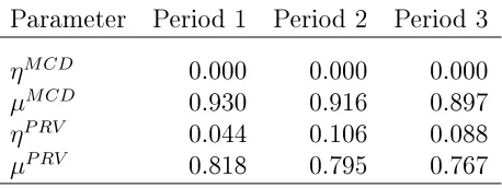
(22) SCHIP was designed to cover uninsured children in families with incomes that are modest but too high to qualify for Medicaid. States are given flexibility in designing their CHIP eligibility requirements and policies within broad federal guidelines. In general, in all states children from birth through age 19 who live in families with incomes above the Medicaid thresholds and up to around 241% of FPL on average are eligible for SCHIP (North Dakota currently has the lowest level at 160% of FPL. New York currently has the highest level at 400% of the FPL.) The Affordable Care Act (ACA, known also as ObamaCare) was enacted in March 2010 and took effect in January 2014.. It increases the level of eligibility for Medicaid. for children of 6-18 years old from 100% of FPL to 133% of FPL (effectively to 138% of FPL due to a special deduction to income of 5% while determining Medicaid eligibility). It expands affordable Medicaid coverage for millions of low-income people that were not eligible for Medicaid before. Adults of the age 19-65 with the income lower than 133% of FPL (which is effectively 138%) now have a chance to get Medicaid in states that expanded Medicaid coverage according to ACA. However, there are some issues with implementation of Obamacare on the state level. States might reject implementation of Medicaid expansion. Now there are 29 states that expand Medicaid and 22 states that do not expand Medicaid. If a person lives in a state that does not expand Medicaid coverage, she still might be able to receive Medicaid if her income is less than 100% of FPL. For the purposes of this chapter I will consider that all adults of the age 19-21 are not different from children of age 6-18 in terms of Medicaid eligibility and have the same 100% FPL eligibility threshold.. Health Insurance in the Model Economy. I model governmental policy with respect to. health in a general way, but try to capture the main features of the current policy in the U.S. If parents have low income, their children are eligible for Medicaid/SCHIP. However, there are some short-cuts I have to make in my model. Actual Medicaid/SCHIP policies have higher threshold to be eligible for Medicaid (133% of FPL) for children between ages 0 to 5 than children of age 6-18 (100% of FPL); and children after age 18 are not eligible. In my model childhood periods are 0-7, 8-14 and 15-21. I assume that health policy does not change within model periods, i.e. those who were eligible until age 5 are still eligible. 8. until age 7. And those who were eligible until age 18 are eligible until age 21.. Parents decide on buying private insurance for their child and on the amount of medical spending, taking into account insurance functions.. Insurance mechanism is similar to. Ozkan (2013). If parents buy private insurance for their child, they pay a tax-deductible insurance premium. 𝑝𝑖𝑛𝑠 . Insurance premium is the same for all children of each cohort but. might be different for different cohorts. I model insurance premium to be tax deductible as around 85% of private insurances are provided through employers. If parental income in period. 𝑗. is lower than the threshold. 𝐼𝑗 ,. the child is eligible for. 9. Medicaid and SCHIP and parent does not have to pay an insurance premium. model insurance functions for private insurance in the same way.. I will. (𝑃 𝑅𝑉 ) and Medicaid/SCHIP (𝑀 𝐶𝐷) 𝜂 𝑀 𝐶𝐷/𝑃 𝑅𝑉 , up to which parents do. Both of them have a deductible. not receive the reimbursement from insurance company/government, and for each dollar. 8 I abstract from eligibility of teenagers and young adults that got pregnant to Medicaid. 9 In the data, being eligible for Medicaid and SCHIP does not mean that people enroll into it. Indeed, 8 million children remain uninsured, including 5 million who are eligible for Medicaid and SCHIP but not enrolled (Medicaid website). In this chapter I will abstract from this fact and assume that if child is Medicaid eligible, he is enrolled into the program, except for the case when parents purchased a private insurance for him.. 21.

(23) above the threshold. 𝜂 𝑀 𝐶𝐷/𝑃 𝑅𝑉 ,. they receive a fraction. 𝜇𝑀 𝐶𝐷/𝑃 𝑅𝑉. as a copayment-rate.. 𝑚 is given. Hence, the amount they receive from the government as a subsidy for spending by. {︃ 𝑀 𝐶𝐷/𝑃 𝑅𝑉 𝜒𝑗 (𝑚). =. 𝑀 𝐶𝐷/𝑃 𝑅𝑉. 0 if 𝑚 ≤ 𝜂𝑗 𝑀 𝐶𝐷/𝑃 𝑅𝑉 𝑀 𝐶𝐷/𝑃 𝑅𝑉 𝜇 (𝑚 − 𝜂𝑗 ). if. .. 𝑀 𝐶𝐷/𝑃 𝑅𝑉. 𝑚 > 𝜂𝑗. Eligibility for Medicaid/SCHIP indicator is given by. ℐ𝑗𝑀 𝐶𝐷 (𝐴𝑇𝑡 (𝐻)) where. 𝐼𝑗. {︂ =. 0 if 𝐴𝑇𝑡 (𝐻) > 𝐼𝑗 , 1 if 𝐴𝑇𝑡 (𝐻) ≤ 𝐼𝑗 .. corresponds to eligibility threshold set up by the Medicaid and SCHIP (which. depends on the age of children), devoted by a parent of age. 𝑡. 𝐴. is the productivity of a parent, and. to the labor market (hence. 𝐴𝑇𝑡 (𝐻). 𝑇𝑡 (𝐻). is hours. is their total income).. 3.3. Household Problem Households maximize their lifetime utility. The discount factor is. 𝛽 < 1.. The per-period. utility from consumption is assumed to take the following functional form. 𝑢(𝑐) =. 𝑐1−𝜎 . 1−𝜎 𝑏=0. I start by describing the problem of parents who are childless, either because. (i.e.. they never had children) or because their children already left the house or are not yet born.. Childless Parents State space of the household without children is given by the current productivity,. 𝐻. is the health status,. child-bearing status of parents.. 𝜃. x = {𝐴, 𝐻, 𝜃, 𝑏}, 𝑏. is marital status, and. where. 𝐴. is. is parental. If a parent does not have any child at home, then she. only consumes. Her value function is given by. 𝑉𝑡,0 (x) = max {𝑢(𝑐) + 𝛽𝐸𝐴′ ,𝐻 ′ 𝑉𝑡+1,𝑗 (x′ )} , subject to. 𝑐 = (1 − 𝜏 )𝑇𝑡 (𝐻)𝐴, and. {︂ 𝑗=. where. 𝜏. 0,. 𝑏 = 0,. or. 𝑏=1. and. 𝑡 > 3,. or. 𝑏=2. and. 𝑡 > 4,. 1, otherwise. is the tax rate,. ,. 𝑇𝑡 (𝐻) is the time that parents devote to labor market as a function (1 − 𝜏 )𝑇𝑡 (𝐻)𝐴, and. of their health. Hence, after-tax income of the household is given by. absent any savings they consume their income in the current period. Note that the value functions of parents are indexed both by their age, a childless parent. 𝑡,. and the age of their children,. 𝑗.. For. 𝑗 = 0.. Next period, the household will have the same values of 𝜃 and 𝑏, but will have new 𝐴 and 𝐻, hence x′ = {𝐴′ , 𝐻 ′ , 𝜃, 𝑏}. A household with no children today can still. draws for. be without any child next period, if. 𝑏 = 0 or the children have already left the house. The 𝑡 = 1 and 𝑏 = 2,. household can also have a 1-year old child next period, if, for example,. i.e. the parents are one-year old and have their children in the second period. The last constraint summarizes how the number of children evolves for the households.. 22.

(24) Parents with Children Consider now the problem of parents with children. We will first start with the problem of a parent whose child is 3 years old and will become adult next period.. We assume. that each period parents with children decide whether to buy health insurance for the next period, except when their children is just born, i.e.. 𝑗 = 1,. in which case they have. to decide whether to buy health insurance for the current as well as the next (second period). As a result, a parent with a 3-year-old child arrives to the current period with heath insurance decision already made last period when the child was two years old. This decision was made before parents observe their own as well as their children heath and ability outcomes for the next period As a result, health insurance decision for the third period is not made conditional on children’s current health. Given this insurance decision from last period, a parent with a 3-years old child decides how much to spend on his child’s health. The parent also decides whether to send her child to college, given government college subsidy program. The problem for a parent with a 2-years-old child is quite similar. Given the insurance decision from last period, parents decide how much to spend on health and education of their children, given available government policies. When a parent has a 1-years old child, then he decides whether to buy health insurance for the current period, again before observing his child’s current health and ability as well as makes a plan whether to buy insurance for the next period after first period health and ability are realized.. Third Period of Childhood. (𝑗 = 3). Given an insurance decision from the last. period, in the third period of the childhood parents take decisions on college education, medical spending, and consumption. expected utility of her adult child.. The parent is altruistic and she cares about the As a result, parents are motivated to leave their. children with highest possible productivity and health. State space of a parent with a child in the third period of childhood in the beginning * * * * of a period is given by x = {𝑎 , ℎ , 𝜃, 𝑏, 𝑎, ℎ, 𝐴, 𝐻}, where 𝑎 and ℎ are children’s innate ability and health,. 𝑎 and ℎ are child’s current ability and health, and 𝐴 and 𝐻. are parents’. current ability and health. Given their insurance status (insured,. 𝑖,. or uninsured,. 𝑢),. parents’ decision whether. to send their children to college is given by the following value function. 𝑐,𝑖 𝑛𝑐,𝑖 𝑖 𝑉𝑡,3 (x) = max{𝑉𝑡,3 (x), 𝑉𝑡,3 (x)}, and. 𝑐,𝑢 𝑛𝑐,𝑢 𝑢 𝑉𝑡,3 (x) = max{𝑉𝑡,3 (x), 𝑉𝑡,3 (x)}, where superscript. 𝑐. corresponds to sending to college, and. 𝑛𝑐. to not sending to college.. The value associated to each of these outcomes reflects optimal decisions by the parents.. The value of sending the child to college and purchasing health insurance, for. example, is given by. {︁ }︁ 𝑐,𝑖 𝑉𝑡,3 (x) = max 𝑢(𝑐) + 𝛽𝐸𝑉𝑡+1,0 (x′ ) + 𝜓𝐸 𝑉ˆ1,𝑗 (x′𝑐ℎ𝑖𝑙𝑑,𝑗 ) , 𝑐,𝑚. where. 𝐸 𝑉ˆ1,𝑗. is the expected value of the child when he becomes adult and child’s state ′ space when she becomes adult, x𝑐ℎ𝑖𝑙𝑑,𝑗 , is defined as her initial productivity level, which is the function 𝑓 (𝑎3 , ℎ3 , 𝑐𝑜𝑙𝑙𝑒𝑔𝑒, 𝜐3 ), her initial health that is the function 𝑔(ℎ3 , 𝑚3 , 𝜀3 ), his marital and child-bearing shock,. 𝜓. is the degree of altruism of a parent, to which extent. he enjoys utility of his child.. 23.

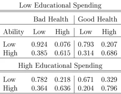
(25) The budget constraint associated to this problem is given by:. 𝑐 = (1 − 𝜏 )[𝑇𝑡 (𝐻)𝐴) − 𝑝𝑖𝑛𝑠 ] − 𝑚 + 𝜒𝑃 𝑅𝑉 (𝑚) − (1 − 𝜅(𝑇𝑡 (𝐻)𝐴))𝐸,. (1.5). and. 𝜅(𝑇𝑡 (𝐻)𝐴) = max{0, 𝐸 − 𝜅(𝐴𝑇𝑡 (𝐻))𝜑 }, where where. 𝑐. is consumption,. 𝜏. is the tax rate,. 𝑇𝑡 (𝐻). is a function of health that. 𝐴 is parent’s productivity, 𝑝𝑖𝑛𝑠 is private insurance 𝑚 is medical spending, 𝜒𝑃 𝑅𝑉 (𝑚) is private insurance reimbursement of medical spending made by parents, 𝐸 is the tuition fee for college, 𝜅(𝑇𝑡 (𝐻)𝐴) is governmental 𝑃 𝑅𝑉 subsidy for college. Hence, the parent has (1 − 𝜏 )[𝑇𝑡 (𝐻)𝐴 − 𝑝𝑖𝑛𝑠 ] +𝜒 (𝑚) as her income determines parental labor supply,. premium,. after paying tax deductible insurance premium and receiving reimbursements from the private insurance company. She spends. 𝑚 on health care of her child and (1−𝜅(𝑇𝑡 (𝐻)𝐴))𝐸. on college. In the same spirit, the value function associated to not sending the child to college and not purchasing private insurance is given by. {︁ }︁ 𝑛𝑐,𝑢 𝑉𝑡,3 (x) = max 𝑢(𝑐) + 𝛽𝐸𝑉𝑡+1,0 (x′ ) + 𝜓𝐸 𝑉ˆ1,𝑗 (x𝑐ℎ𝑖𝑙𝑑,𝑗 ) , 𝑐,𝑚. subject to:. 𝑐 = (1 − 𝜏 )[𝑇𝑡 (𝐻)𝐴 + 𝑡3 (ℎ)𝑎] − 𝑚 + 𝜒𝑀 𝐶𝐷 (𝑚)ℐ3𝑀 𝐶𝐷 (𝑇𝑡 (𝐻)𝐴), where. (1.6). 𝑡3 (ℎ)𝑎. is child’s hours supplied to the labor market (child works if he does not 𝜒𝑀 𝐶𝐷 (𝑚)ℐ3𝑀 𝐶𝐷 (𝑇𝑡 (𝐻)𝐴) is reimbursement of medical spending by 𝑀 𝐶𝐷 Medicaid in case child is Medicaid-eligible, i.e. if ℐ3 (𝑇𝑡 (𝐻)𝐴) = 1.. attend college) and. Second Period of Childhood. (𝑗 = 2). As in the third period of childhood, par-. ents arrive to the second period of childhood with an insurance decision from the last period.. Then they decide on medical and educational spending and consumption as. well as whether to buy insurance for the next period.. State space of a parent with. a child in the second period of childhood in the beginning of a period is given by x = {𝑎, ℎ, 𝑎* , ℎ* , 𝐴, 𝐻, 𝜃, 𝑏}. Then, the value function for an insured child is given by. {︀ }︀ 𝑖 𝑖 𝑢 𝑉𝑡,2 (x) = max 𝑢(𝑐) + 𝛽 max{𝐸𝐴′ ,𝐻 ′ ,𝑎′ ,ℎ′ 𝑉𝑡+1,3 (x′ ), 𝐸𝐴′ ,𝐻 ′ ,𝑎′ ,ℎ′ 𝑉𝑡+1,3 (x′ ) }, 𝑐,𝑒,𝑚. subject to. 𝑐 = (1 − 𝜏 )[𝐴𝑇𝑡 (𝐻) − 𝑝𝑖𝑛𝑠 ] − 𝑚 + 𝜒𝑃 𝑅𝑉 (𝑚) − 𝑒, 𝑎′ = 𝑓 (𝑎, ℎ, 𝑒, 𝜐),. and. 𝑒≥𝑔. ℎ′ = 𝑔(ℎ, 𝑚, 𝜀) and. 𝑄𝑡𝐻 ′ |𝐻 ,. and. 𝑒 is parental educational spending, 𝑔 is governmental spending on secondary educa𝑄𝑡𝐻 ′ |𝐻 and 𝑄𝑡𝐴′ |𝐴 are exogenous stochastic process that captures parental health and. where tion,. 𝑄𝑡𝐴′ |𝐴 .. 24.

(26) productivity life-cycle profiles. The terms. 𝑖 𝑢 𝐸𝐴′ ,𝐻 ′ ,𝑎′ ,ℎ′ 𝑉𝑡+1,3 (x′ ) and 𝐸𝐴′ ,𝐻 ′ ,𝑎′ ,ℎ′ 𝑉𝑡+1,3 (x′ ) rep-. resent the expected value of being insured or uninsured in the third period of childhood, respectively. The value function for an uninsured child is given by. {︀ }︀ 𝑢 𝑖 𝑢 𝑉𝑡,2 (x) = 𝐸max 𝑢(𝑐) + 𝛽 max{𝐸𝐴′ ,𝐻 ′ ,𝑎′ ,ℎ′ 𝑉𝑡+1,3 (x′ ), 𝐸𝐴′ ,𝐻 ′ ,𝑎′ ,ℎ′ 𝑉𝑡+1,3 (x′ ) }, 𝑐,𝑒,𝑚. subject to. 𝑐 = (1 − 𝜏 )[𝐴𝑇𝑡 (𝐻)] − 𝑚 + 𝜒𝑀 𝐶𝐷 (𝑚)ℐ2𝑀 𝐶𝐷 (𝐴𝑇𝑡 (𝐻)) − 𝑒, 𝑎′ = 𝑓 (𝑎, ℎ, 𝑒, 𝜐), and 𝑒 ≥ 𝑔, ℎ′ = 𝑔(ℎ, 𝑚, 𝜀), and. 𝑄𝑡𝐻 ′ |𝐻 , where. ℐ2𝑀 𝐶𝐷 (𝐴𝑇𝑡 (𝐻)). and. 𝑄𝑡𝐴′ |𝐴 .. is the indicator function for Medicaid eligibility in the period 2.. First Period of Childhood (𝑗 = 1). Parents with a one-year-old child decide first. whether to buy insurance for the current period. Then they decide how much to spend on education and health of their children as well as whether to buy insurance for the next ̃︀ = {𝜃, 𝑏, 𝐴, 𝐻, 𝐴* , 𝐻 * }. period. At the start of the period, parents’ state space is given by x Hence they do not know yet period. Then on. 𝑒, 𝑚. 𝑎. and. ℎ. 𝑎. or. ℎ,. and decide whether to buy insurance for the current. are realized and, given their health insurance decisions they decide. and purchasing or not an insurance for the second period. The state space of the. parent after the realization of. 𝑎 and ℎ is denote by x = {𝜃, 𝑏, 𝐴, 𝐻, ℎ, 𝑎}. Hence the health. insurance decision of parents at the start of the period is characterized by the following value function. 𝑖 𝑢 𝑉𝑡,1 (̃︀ x) = max{𝐸ℎ,𝑎 𝑉𝑡,1 ((x),𝐸ℎ,𝑎 𝑉𝑡,1 (x)}, * * * where the expectations on 𝑎 and ℎ are conditional on 𝐴 and 𝐻 (recall that 𝑎 = 𝑎 and ℎ = ℎ* in the first period of childhood and the innate health and ability are correlated across generations). Once. ℎ. and. 𝑎. are realized the problem of parent with a one-year-old. child looks very similar to the problem of parents with a two-years-old child. For parents with health insurance, it is given by. {︀ }︀ 𝑖 𝑖 𝑢 𝑉𝑡,1 (x) = max 𝑢(𝑐) + 𝛽 max{𝐸𝐴′ ,𝐻 ′ ,𝑎′ ,ℎ′ 𝑉𝑡+1,2 (x′ ), 𝐸𝐴′ ,𝐻 ′ ,𝑎′ ,ℎ′ 𝑉𝑡+1,2 (x′ ) }, 𝑐,𝑒,𝑚. subject to. 𝑐 = (1 − 𝜏 )[𝐴𝑇𝑡 (𝐻) − 𝑝𝑖𝑛𝑠 ] − 𝑚 + 𝜒𝑃 𝑅𝑉 (𝑚) − 𝑒, 𝑎′ = 𝑓 (𝑎, ℎ, 𝑒, 𝑔, 𝜐),. and. 𝑒≥𝑔. ℎ′ = 𝑔(ℎ, 𝑚, 𝜀), and. 𝑄𝑡𝐻 ′ |𝐻 ,. and. 25. 𝑄𝑡𝐴′ |𝐴 ..

(27) For parents without health insurance, the problem reads as. }︀ {︀ 𝑢 𝑖 𝑢 𝑉𝑡,1 (x) = 𝐸max 𝑢(𝑐) + 𝛽 max{𝐸𝐴′ ,𝐻 ′ ,𝑎′ ,ℎ′ 𝑉𝑡+1,2 (x′ ), 𝐸𝐴′ ,𝐻 ′ ,𝑎′ ,ℎ′ 𝑉𝑡+1,2 (x′ ) }, 𝑐,𝑒,𝑚. subject to. 𝑐 = (1 − 𝜏 )[𝐴𝑇𝑡 (𝐻)] − 𝑚 + 𝜒𝑀 𝐶𝐷 (𝑚)ℐ2𝑀 𝐶𝐷 (𝐴𝑇𝑡 (𝐻)) − 𝑒,. 𝑎′ = 𝑓 (𝑎, ℎ, 𝑒, 𝑔, 𝜐), and 𝑒 ≥ 𝑔,. ℎ′ = 𝑔(ℎ, 𝑚, 𝜀), and. 𝑄𝑡𝐻 ′ |𝐻 , and 𝑄𝑡𝐴′ |𝐴 .. 4. Estimation To estimate the model I adopt a two-step procedure similar to the one used by Gourinchas and Parker (2002), De Nardi, French and Jones (2010a), and Coşar, Guner and Tybout (2016). In the first step I select all parameters that could be assigned without simulating the model (either directly from the data or from previous literature). Most importantly, characteristics of public and private insurance schemes, and life cycle health profiles of adults are set in the first step. In the second step, I estimate the rest of the parameters with method of simulated moments, taking the first-step estimates as given. In this section I describe first step estimates, then I turn to the second step estimation.. 4.1. First-step estimation Few parameters can be determined based on available estimates in the literature or can be calculated directly from aggregate statistics.. Discount factor, 𝛽 .. I choose discount factor to be the standard value, 0.96 per year,. from the literature.. Coefficient of relative risk-aversion, 𝜎.. Coefficient of relative risk-aversion is. taken from De Nardi et al. (2010a) and is equal to 3.. Government spending for education, 𝑔.. According to Digest of Education Statis-. tics, total expenditures per pupil in public elementary and secondary schools in 2010-2011 is $12,908.. 10. Variance of health shocks, 𝜎𝜐 , and variance of ability shocks in the first and second periods, 𝜎𝜀 . As production functions are logits, variances are normalized to. 𝜋 2 /3.. Several other parameters are estimated directly using micro data.. 10 Source:. http://nces.ed.gov/programs/digest/d13/tables/dt13_236.55.asp.. diture per pupil in average daily attendance. 26. Variable Expen-.