ENVIRONMENTAL RISK ASSESSMENT IN THE MEDITERRANEAN REGION USING ARTIFICIAL NEURAL NETWORKS
Marelys Josefina Mújica Chacín
Dipòsit Legal: T. 1057-2012
ADVERTIMENT. L'accés als continguts d'aquesta tesi doctoral i la seva utilització ha de respectar els drets de la persona autora. Pot ser utilitzada per a consulta o estudi personal, així com en activitats o materials d'investigació i docència en els termes establerts a l'art. 32 del Text Refós de la Llei de Propietat Intel·lectual (RDL 1/1996). Per altres utilitzacions es requereix l'autorització prèvia i expressa de la persona autora. En qualsevol cas, en la utilització dels seus continguts caldrà indicar de forma clara el nom i cognoms de la persona autora i el títol de la tesi doctoral. No s'autoritza la seva reproducció o altres formes d'explotació efectuades amb finalitats de lucre ni la seva comunicació pública des d'un lloc aliè al servei TDX. Tampoc s'autoritza la presentació del seu contingut en una finestra o marc aliè a TDX (framing). Aquesta reserva de drets afecta tant als continguts de la tesi com als seus resums i índexs.
ADVERTENCIA. El acceso a los contenidos de esta tesis doctoral y su utilización debe respetar los derechos de la persona autora. Puede ser utilizada para consulta o estudio personal, así como en actividades o materiales de investigación y docencia en los términos establecidos en el art. 32 del Texto Refundido de la Ley de Propiedad Intelectual (RDL 1/1996). Para otros usos se requiere la autorización previa y expresa de la persona autora. En cualquier caso, en la utilización de sus contenidos se deberá indicar de forma clara el nombre y apellidos de la persona autora y el título de la tesis doctoral. No se autoriza su reproducción u otras formas de explotación efectuadas con fines lucrativos ni su comunicación pública desde un sitio ajeno al servicio TDR. Tampoco se autoriza la presentación de su contenido en una ventana o marco ajeno a TDR (framing). Esta reserva de derechos afecta tanto al contenido de la tesis como a sus resúmenes e índices.
Marelys Josefina Mujica Chacín
ENVIRONMENTAL RISK ASSESSMENT
IN THE MEDITERRANEAN REGION
USING ARTIFICIAL NEURAL NETWORKS
DOCTORAL DISSERTATION
Marelys Josefina Mujica Chacín
ENVIRONMENTAL RISK ASSESSMENT IN
THE MEDITERRANEAN REGION USING
ARTIFICIAL NEURAL NETWORKS
DOCTORAL DISSERTATION
Directed by Dr. Francesc Giralt and Dr. Robert Rallo
Departament d’Enginyeria Química
Universitat Rovira i Virgili Departament d’Enginyeria Química
Campus Sescelasdes, Av. Països Catalans 26, 46007 Tarragona, Spain
Tel: 977559700 Fax: 977559699
We, Dr. Francesc Giralt I Prat and Dr. Robert Rallo Moya, members of the Department of Chemical Engineering of the Universitat Rovira I Virgili,
CERTIFY:
That the present study, entitled “ENVIRONMENTAL RISK ASSESSMENT IN THE MEDITERRANEAN REGION USING ARTIFICIAL NEURAL NETWORKS” presented by Marelys Josefina Mujica Chacín, in partial fulfillment of the requirements for the degree of Doctor, has been carried out under our supervision at the Department of Chemical Engineering of this university and meets the requirements to obtain the European Mention.
Tarragona, February 20th 2012.
A Diego,
Acknowledgments
I would like to thank to my supervisors Dr. Francesc Giralt and Dr. Robert Rallo for their
guidance, support and advices. Also, special thanks to Dr. Gabriela Espinosa for her
support, guidance and help during the first years of this project.
To my PhD partners, my lab’s colleagues and the personnel of chemical engineering
department of URV for the nice talks during coffee breaks and “hall-talks”. Been grateful
by all good friends that URV doctoral program made me find and who will remain
forever… mi familia de Tarragona!
Special thanks to my family, my parents Miguel and Etel, my brothers Migue and
Fernando and my sister Gaby for encourage me to successfully finish this thesis.
Also, I’m infinitely grateful of my lovely husband Diego and my daughters Ana Mercedes
and Alba Cecilia for their unconditional support and patience during my doctoral studies.
For the financial support, I want to acknowledge to the European Union (NoMiracle
Project, European Commission, FP6 Contract No. 003956), and Servei de Gestió de la
Recerca and Agència de Gestió d'Ajuts Universitarisi de Recerca (AGAUR) of Generalitat
Resumen
Existe una creciente preocupación de nuestra sociedad sobre aspectos medioambientales como el cambio climático, la pérdida del hábitat, la deposición ácida, el descenso de la diversidad biológica y los impactos ecológicos de compuestos contaminantes como pesticidas y químicos tóxicos. El análisis de riesgo medioambiental puede ayudar a identificar estos problemas, establecer prioridades y proveer bases científicas para acciones regulatorias.
La realización de un estudio satisfactorio de estos y otros problemas medioambientales, requiere el uso de herramientas inteligentes que sean capaces de visualizar y extraer relaciones entre fuentes antropogénicas y sus efectos sobre el medio. Los desafíos principales relacionados a la aplicación de éstas técnicas son la naturaleza altamente no lineal de las relaciones causa – efecto estudiadas, así como la falta de información geográfica confiable. Los algoritmos de aprendizaje de máquinas y las técnicas de búsqueda de datos han probado ser muy exitosos en aplicaciones que incluye el manejo de datos de altas dimensiones y la presencia de incertidumbre.
Los mapas auto-organizados han demostrado ser una herramienta apropiada para la clasificación y visualización de grupos de datos complejos. Redes neuronales, como los mapas auto-organizados (SOM) o las redes difusas ARTMAP (FAM), se utilizan en este estudio para evaluar el impacto medio ambiental acumulativo en diferentes medios (aguas subterráneas, aire y salud humana). Los SOMs también se utilizan para generar mapas de concentraciones de contaminantes en aguas subterráneas simulando las técnicas geostadísticas de interpolación como kriging y cokriging. Para evaluar la confiabilidad de las metodologías desarrolladas en esta tesis, se utilizan procedimientos de referencia como puntos de comparación: la metodología DRASTIC para el estudio de vulnerabilidad en aguas subterráneas y el método de interpolación espacio-temporal conocido como Bayesian Maximum Entropy (BME) para el análisis de calidad del aire.
Summary
Our society is increasingly aware of environmental issues including climate change, habitat loss, acid deposition, a decrease in biological diversity, and the ecological impacts of xenobiotic compounds such as pesticides and toxic chemicals. Environmental risk assessment (ERA) can help identify these environmental problems, establish priorities, and provide a scientific basis for regulatory actions.
A successful assessment of these and other environmental problems requires the use of intelligent tools capable of visualizing and extracting causal relationships among stressors and their effects. The main challenges related to the application of these techniques are the highly non-linear nature of the relationships between stressor and their effects as well as the lack of reliable and geographically distributed data. Machine learning algorithms and data-mining techniques have proven to be very successful in applications that include the management of high dimensional datasets and the presence of uncertainty.
The self-organizing map algorithm has demonstrated to be an appropriate tool for the classification and visualization of complex datasets. Neural networks, such as Self-Organizing Maps (SOM) or Fuzzy ARTMAP (FAM), are used to address cumulative environmental impact in different media (groundwater, air and human health). SOMs are also used to generate pollutant concentration maps in groundwater by simulating the kriging and co-kriging interpolation methodology. In order to evaluate the reliability of the methodologies developed in this thesis, well-known reference approaches were performed for comparison purposes: DRASTIC index for groundwater vulnerability assessment and Bayesian Maximum Entropy (BME) for air quality assessment.
Contents
Page
Chapter 1 Introduction 1
1.1 Motivation 2
1.2 Hypothesis and objectives 4
1.3 Scientific contributions 5
1.4 Organization of the manuscript 6
Chapter 2 Background Concepts 7
2.1 Environmental risk assessment 8
2.2 Groundwater vulnerability 9
2.2.1 DRASTIC vulnerability index 11
2.3 Spatial interpolations 13
2.3.1 Geostatistics 13
2.3.2 Bayesian maximum entropy 17
2.4 Artificial neural networks 20
2.4.1 Feed-forward neural networks 21
2.4.2 Radial basis functions networks 22
2.4.3 Self-organizing maps 23
2.4.4 Recurrent neural networks 26
2.4.5 Fuzzy ARTMAP neural network 26
2.5 References 28
Chapter 3 Groundwater Vulnerability Assessment 33
3.1 Introduction 33
3.2 Area of study and data 36
3.2.1 Regional scale: Catalonia 37
3.2.2 Local scale: Camp de Tarragona 38
3.2.3 Pollution data 41
3.3 Local scale vulnerability assessment: Camp de Tarragona 43
3.3.1 Cumulative pollution maps 43
3.3.2 DRASTIC-based intrinsic vulnerability map 46
3.3.3 SOM-based vulnerability map 57
3.4 Vulnerability assessment at regional scale: Catalonia 66
3.4.1 Cumulative pollution maps 66
3.4.2 DRASTIC vulnerability model 69
3.5 Conclusions 74
3.6 References 75
Chapter 4 Lead Exposure Assessment 81
4.1 Introduction 81
4.2 Area of study and data 82
4.3 SOM for variable selection 84
4.4 Fuzzy ARTMAP for lead exposure assessment 86
4.5 Conclusions 89
4.6 References 90
Chapter 5 Spatio-temporal Air Quality Assessment 91
5.1 Introduction 91
5.2 Area of study and data 96
5.3 Spatio-temporal mapping 102
5.3.1 BME approach 102
5.3.2 SOM approach 106
5.4 Conclusions 111
5.5 References 112
Chapter 6 Human Health Risk Assessment 115
6.1 Introduction 115
6.2 Area of study and data 116
6.3 Evaluation of SOM capabilities in HHRA 121
6.3.1 Concentrations maps using SOM 121
6.3.2 Risk maps using SOM 123
6.4 Conclusions 125
6.5 References 126
Chapter 7 Conclusions 129
7.1 Main conclusions 129
7.2 Summary of data-driven ANN methodology in ERA 131
7.3 Research opportunities 132
Annex A Research Contributions 133
A.1 Paper on DRASTIC-SOM for Camp de Tarragona 135
A.2 Paper on SOM-based vulnerability in the Mediterranean region 153
Annex B Matlab’s Toolboxes Description 191
B.1 SOM Toolbox in Matlab 193
List of Figures
[image:15.595.87.531.94.768.2]Page
Figure 2.1. Theoretical Variogram parameters. Range (a), Sill (C) and Nugget (C0) 14
Figure 2.2. Theoretical variogram models (Spherical, Gaussian and Exponential) 16
Figure 2.3. Simple neuron model in an ANN 20
Figure 2.4. Multilayer perceptron feed-forward neural network architecture 21
Figure 2.5. Neighborhoods (levels 0, 1 and 2) of unit (0) in (left) rectangular and (right)
hexagonal lattices 23
Figure 2.6. Best matching unit (BMU) and its topological neighbors (black dots) are updated during the SOM training process. Black and gray circles depict changes in location
caused by the updating process 23
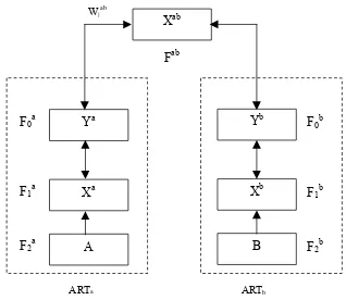
Figure 2.7. Fuzzy ARTMAP network architecture 27
Figure 3.1. Spatial location of the area of study. (a) Regional scale: Catalonia. (b) Local scale:
Camp de Tarragona 37
Figure 3.2. Catalonia Digital Terrain Model 39
Figure 3.3. Catalonia Land uses map 39
Figure 3.4. Camp de Tarragona Digital Terrain Model 40
Figure 3.5. Camp de Tarragona Geological Map 40
Figure 3.6. Camp de Tarragona Land uses map 40
Figure 3.7. Groundwater quality control points in Catalonia area 41
Figure 3.8. Spatial distribution of nitrates concentration generated by kriging interpolation in a
two-year period. (a) year 2002, (b) year 2004 44
Figure 3.9. Smooth cumulative exposure maps. Combined effect of water pollutants exceeding regulatory thresholds. (left) Year 2002: Pb, Fe, Mn, Ba and Nitrates. (right) Year 2004: Pb, Fe, Mn, Ba, Al, Se, Nitrates and Nitrites. The numbers in the labels
indicate the number of pollutants exceeding legal threshold values 45
Figure 3.10. Point cumulative exposuremaps. Combined effect of water pollutants exceeding regulatory thresholds (left) year 2002; (right) year 2004. The numbers in the labels
indicate the number of pollutants exceeding legal threshold values 46
Figure 3.11. DRASTIC features generation from hydrogeological and climate data 46
Figure 3.12. Depth to water layer for DRASTIC Index 47
Figure 3.13. Net Recharge layer for DRASTIC Index 48
Figure 3.14. Aquifer Media layer for DRASTIC Index 48
Figure 3.15. Soil Media layer for DRASTIC Index 49
Figure 3.16. Topography layer for DRASTIC Index 49
Figure 3.17. Impact of vadose zone ratting for DRASTIC Index 50
Figure 3.18. Hydraulic Conductivity layer for DRASTIC Index 51
Figure 3.19. DRASTIC vulnerability maps for Camp de Tarragona at different vulnerability classes
definitions: (a) Aller, (b) Draoui and (c) Ahmed 53
Figure 3.20. Case study definitions for DRASTIC-based SOM intrinsic vulnerability model. (vI:
Figure 3.21. DRASTIC-based SOM intrinsic vulnerability model. (left) U-Matrix and c-planes for the seven DRASTIC features (D, depth to water; R, net recharge; A, aquifer media; S, soil media; T, topography; I, impact of vadose zone; C, hydraulic conductivity);
(right) DRASTIC-based SOM vulnerability map for the Camp de Tarragona 60
Figure 3.22. SOM-based specific vulnerability model (left) U-Matrix and C-planes for the seven input variables considered in the current SOM model (H, piezometric level; P, annual rainfall; Ks, soil permeability; %s, land surface slopes; Ka, hydraulic conductivity of the aquifer; land, land use); (right) SOM specific vulnerability map
for the Camp de Tarragona 62
Figure 3.23. Scheme of the SOM-based specific vulnerability methodology 65
Figure 3.24. Spatial distribution of nitrate concentrations for year 2002 generated by (up)
kriging interpolation (down) SOM interpolation 67
Figure 3.25. Cumulative exposure map for Catalonia in year 2002 generated by (up) kriging interpolation, and (down) SOM interpolation. Combined effect of water pollutants exceeding regulatory thresholds (Pb, Fe, Mn, Se, sulfate and nitrate).The numbers
in the labels indicate the number of pollutants exceeding legal threshold values 68
Figure 3.26. DRASTIC vulnerability map for Catalonia 70
Figure 3.27. SOM-based Specific vulnerability map for Catalonia. The variables used to characterize vulnerability are piezometrics, annual rainfall, soil’s permeability,
surface slopes, aquifer media, hydraulic conductivity, and land uses 71
Figure 3.28. (left) Zoom of Catalonia SOM-based specific vulnerability map; (right) Camp de
Tarragona SOM-based specific vulnerability map 73
Figure 4.1. Hydrogeological areas in Catalonia region 83
Figure 4.2. Industrial areas and principal roads in Catalonia region for year 2002 83
Figure 4.3. Lead measurement points in Catalonia for year 2002 with “detected” value of lead
concentration 84
Figure 4.4. U-Matrix (upper -left corner) and distribution in the output space of input variables
in the trained SOM 85
Figure 4.5. Test and training data sets classification by SOM 86
Figure 4.6. Input and output parameters for training a Neural Networks 87
Figure 4.7. Fuzzy ARTMAP (left) and Backpropagation (right) neural networks crossplots for
lead concentration (µg/l) in Catalonia area 87
Figure 4.8. Fuzzy ARTMAP test predictions for Lead concentrations in Catalonia area 88
Figure 4.9. Backpropagation network test predictions for Lead concentrations in Catalonia area 88
Figure 5.1. Principal anthropogenic pollution sources of PM10 in Catalonia at year 2007. The
number above each bar indicates the actual number of pollutant sources. Red circles represent pollution sources due to gas/fuel distribution and size is
proportional to number of stations 95
Figure 5.2. PM10 emissions for year 2004 reported in the Spanish register of emissions and
pollutant sources, PRTR Spain. (Size and color of circles are proportional to level of
emissions) 95
Figure 5.3. Principal roads/highways (black lines) and daily automotive traffic reported at measurements stations in Catalonia for study years (2003 – 2007). (Source:
Departament de Política Territorial i ObresPúbliquesfromGeneralitat de Catalonia) 96
Figure 5.4. PM10 monitoring stations in Catalonia over the period of study (2003-2007) 96
Figure 5.5. Spatial distribution of monitoring stations: based on the number of daily measurements (Ndm). Measurements stations with 80 or more daily measures
interpolation
Figure 5.6. Distribution of the number of daily measurements (Ndm) in monitoring stations at
each study year (2003-2007) 98
Figure 5.7. Distribution of PM10 concentrations in Catalonia at each study year (2003-2007) 99
Figure 5.8. Distribution of logarithm of PM10 concentrations in Catalonia at each study year
(2003-2007) 99
Figure 5.9. LogPM10 measurements for years 2003 to 2007 (blue cross), 30-days moving average of logPM10 (red line) and histogram of available data for monitoring station
55 (Barcelona- Gracia-SantGervasi) 100
Figure 5.10. LogPM10 measurements for years 2003 to 2007 (blue cross), 30-days moving
average of logPM10 (red line) and histogram of available data for monitoring station
10 (Tarragona - Port) 100
Figure 5.11. Distribution of PM10 monitoring stations across Catalonia at each study year
(2003-2007) as indicator of exceeding annual limit value (40 µg/m3) 101
Figure 5.12. Soft probabilistic data of logPM10 in monitoring station 55 (Barcelona-
Gracia-SantGervasi). Dashed line is the regulatory limit (log[40 µg/m3]=3.7) 103
Figure 5.13. Soft probabilistic data of logPM10 in monitoring station 10 (Tarragona - Port).
Dashed line is the regulatory limit (log[40 µg/m3]=3.7) 103
Figure 5.14. BME PM10 interpolation over Catalonia at years 2003-2007 105
Figure 5.15. Cumulative density function for original data (blue line) and T-SOM-case 1
predictions (red line) at each study year (2003-2007) 108
Figure 5.16. PM10 interpolation over Catalonia by T-SOM model (Case1) 108
Figure 5.17. PM10 interpolation over Catalonia by T-SOM-BMUs (Case 5) 110
Figure 6.1. Territorial division of Catalonia (blue) county division (black) municipal division 117
Figure 6.2. Distribution of the number of 0-14 years old habitants in Catalonia area by
municipal division (years 2004 and 2005) 117
Figure 6.3. Distribution of number of hospital admissions by asthma in the age range 0-14 in
Catalonia area for year 2004 119
Figure 6.4. Distribution of number of hospital admissions by asthma in the age range 0-14 in
Catalonia area for year 2005 119
Figure 6.5. Air quality measurements stations considered in the HHRA for Catalonia area 120
Figure 6.6. Training variables to produce pollutants concentrations maps using self-organizing
maps 121
Figure 6.7. O3 interpolation in Catalonia area for year 2004 by SOM (left) U-matrix and
C-planes (right) SOM-O3 concentrations map 122
Figure 6.8. O3 interpolation in Catalonia area for year 2005 by SOM (left) U-matrix and
C-planes (right) SOM-O3 concentrations map 123
Figure 6.9. Scheme of SOM-based risk maps for asthma exacerbation due to air pollution in
0-14 years old population 123
Figure 6.10. Children asthma attacks hospital admissions and air pollution relationship in Catalonia area for year 2004 (left) U-matrix and C-planes (right) SOM risk map
model 124
Figure 6.11. Children asthma attacks hospital admissions and air pollution relationship in Catalonia area for year 2005 (left) U-matrix and C-planes (right) SOM risk map
model 125
[image:17.595.84.524.71.776.2]List of Tables
Page
Table 2.1. Overlay and index methods for groundwater vulnerability assessment 10
Table 2.2. DRASTIC weights by Aller et al. (1987) 12
Table 2.3. Examples of general knowledge G bases 18
Table 2.4. Activations functions used in ANN 21
Table 2.5. Radial basis functions 22
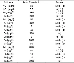
Table 3.1. Regulatory limits for pollutants in drinking water 34
Table 3.2. Sources and resolution of hydrogeological data 38
Table 3.3. Statistics of heavy metals and pesticides in groundwater at year 2002 42
Table 3.4. Statistics of heavy metals and pesticides in groundwater at year 2004 42
Table 3.5. Frequency of annual pollutant concentration exceeding regulatory threshold at
Camp de Tarragona at years 2002 and 2004 45
Table 3.6. Depth to water rating for DRASTIC Index 47
Table 3.7. Ratings for R calculation using equation 3.1 47
Table 3.8. Net Recharge rating for DRASTIC Index 48
Table 3.9. Aquifer Media ratting for DRASTIC Index 48
Table 3.10. Topography ratting for DRASTIC Index 49
Table 3.11. Factors for Vadose Zone estimation 50
Table 3.12. Impact of vadose zone ratting for DRASTIC Index 50
Table 3.13. Hydraulic Conductivity rating for DRASTIC Index 51
Table 3.14. DRASTIC vulnerability classes by (Aller et. al., 1987) 52
Table 3.15. DRASTIC vulnerability classes by (Draoui, et. al., 2008) 52
Table 3.16. DRASTIC vulnerability classes by (Ahmed, 2009) 52
Table 3.17. Frequency of exceeding cumulative legal threshold by year and vulnerability class in
DRASTIC-Aller vulnerability map 55
Table 3.18. Frequency of exceeding cumulative legal threshold by year and vulnerability class in
DRASTIC-Draoui vulnerability map 55
Table 3.19. Frequency of exceeding cumulative legal threshold by year and vulnerability class in
DRASTIC-Ahmed vulnerability map 55
Table 3.20. DRASTIC-Aller statistics for NO
3 in Camp de Tarragona area for years 2002 and 2004 56
Table 3.21. DRASTIC-Draoui statistics for NO
3 in Camp de Tarragona 56
Table 3.22. DRASTIC-Ahmed statistics for NO
3 in Camp de Tarragona area 56
Table 3.23. Vulnerability index categories 59
Table 3.24. Frequency of exceeding cumulative legal threshold by year and intrinsic
vulnerability class in DRASTIC-based SOM vulnerability map 59
Table 3.25. DRASTIC-based SOM statistics for NO3 in Camp de Tarragona area for years 2002
and 2004 60
Table 3.26. Regional maximum and minimum groundwater vulnerabilities for the SOM-based
vulnerability features and analysis 62
[image:18.595.75.522.111.787.2]SOM-based vulnerability map
Table 3.28. SOM-based specific vulnerability map statistics for NO3 in Camp de Tarragona area
for years 2002 and 2004 64
Table 3.29. Frequency of exceeding cumulative legal threshold for each DRASTIC vulnerability
class for Catalonia in 2002 70
Table 3.30. DRASTIC vulnerability map statistics for NO3 in Catalonia at year 2002 70
Table 3.31. Frequency of exceeding cumulative legal threshold at year 2002 and vulnerability
class in SOM-based vulnerability map for Catalonia area 72
Table 3.32. SOM-based specific vulnerability map statistics for NO3 at year 2002 in Catalonia
area 72
Table 4.1. Training and test errors for Fuzzy Art Map and Backpropagation neural networks
for Lead concentrations in Catalonia area 88
Table 5.1. Particulate matter (PM) standards in Spain, including total suspended particulate
matter (TSP) 91
Table 5.2. Statistics of industrial sources of PM10 in Catalonia in 2007 94
Table 5.3. Population distribution over Catalonia in 2006 (Source: IDESCAT,
Institutd’Estadística de Catalonia) 94
Table 5.4. Number of monitoring stations (N) and daily PM10 measurements (Ndm) in the
period 2003-2007. (Percentage of annual data, based on a 365-days year) 97 Table 5.5. Main statistics of PM10 daily average data at study period 2003-2007 97
Table 5.6. Exponential covariance parameters cases for PM10 104
Table 5.7. Main statistics of PM10 interpolated data by BME 104
Table 5.8. T-SOM interpolation total error for the different cases 107
Table 5.9. Main statistics of PM10 interpolated data by T-SOM case 1 107
Table 5.10. T-SOM-BMUs interpolation total error for different input vectors 109
Table 5.11. Main statistics of PM10 interpolated data by T-SOM-BMUs case 5 109
Table 6.1. Air pollutants values in Spain for the protection of human health 116
Table 6.2. Number of habitants by age range in Catalonia at years 2004 and 2005 117
Table 6.3. Distribution of number of hospitalization by respiratory diseases by age range in
Catalonia at years 2004 and 2005 118
Table 6.4. Distribution of number of hospitalization by asthma by age range in Catalonia at
years 2004 and 2005 118
Table 6.5. Distribution of number of hospitalization by heart disease by age range in Catalonia
at years 2004 and 2005 118
Table 6.6. Main statistics of health–related air pollutants annual concentrations for year 2004 120
Table 6.7. Main statistics of health–related air pollutants annual concentrations for year 2005 120
Table 6.8. Minimum and maximum numbers of frequency of exceeding human health
List of Abbreviations
%s Land surface slopes
A Aquifer media – DRASTIC rated
ACA Catalan water agency (Agència Catalana de l’Aigua) Al Aluminium
ANN Artificial Neural Network ART Adaptive Resonance Theory As Arsenic
Ba Barium
BME Bayesian Maximum Entropy
BMU Best Matching Unit in a trained self-organizing map C Hydraulic conductivity of the aquifer – DRASTIC rated
Cd Cadmium
CDF Cumulative Distribution Function
CHEBRO Ebro river agency (Confederación Hidrográfica del Ebro) C-planes Components planes of trained self-organizing map
Cr Chrome
Cu Cooper
D Depth to water table – DRASTIC rated
EPA United States Environmental Protection Agency ERA Environmental Risk Assessment
EU European Union
FAM Fuzzy ART Map neural network
Fe Lead
FFN Feed-Forward neural Network
GENCAT Catalonia government (Generalitat de Catalunya) GIS Geographic Information Systems
H Piezometric level
HHRA Human Health Risk Assessment
I Impact of vadose zone – DRASTIC rated
ICC Catalan cartographic institute (Institut Cartogràfic de Catalunya) IGME Spanish geologic institute (Instituto Geológico y Minero de España) IK Indicator Kriging
Ka Hydraulic conductivity of the aquifer Ks Soil’s permeability
land Soil uses map (land uses) MAE Mean arithmetic error Max Maximum value Mean Mean arithmetic value Min Minimum value
Mo Molybdenum mse Mean standard error
Ndm Number of daily measurements Ni Nickel
NO2 Nitrate
NO3 Nitrite
OK Ordinary Kriging
O3 Ozone
P Annual rainfall
Pb Lead
PDF Probability Density Function
PRTR Spanish register of emissions and pollutant sources PM Particulate Matter
PM10 Particulate matter of diameter bellow than 10 micrometers
PM2.5 Particulate matter of diameter bellow than 2.5 micrometers
qe Quantization error of SOM Q1 25th quartile
Q3 75th quartile
R Net recharge – DRASTIC rated RBFN Radial Basis Function neural Network RNN Recurrent Neural Network
S Soil media – DRASTIC rated ST Spatio-temporal
S/TRF Space/Time Random Field
Sb Antimony
Se Selenium SK Simple Kriging SO4 Sulfates
SOM Self-Organizing Map std Standard deviation
T Topography – DRASTIC rated te Topology error of the SOM T-SOM Temporal Self-Organizing Map TSP Total Suspended Particles UK Universal Kriging
UB Universitat de Barcelona
U-matrix Unified distance matrix of trained self-organizing map US United States
UTM Universal Transverse Mercator coordinate system vIndex Vulnerability index
Chapter 1
Introduction
Our society is increasingly aware of environmental issues including climate change, habitat loss, acid deposition, a decrease in biological diversity, and the ecological impacts of xenobiotic compounds such as pesticides and toxic chemicals. Environmental risk assessment can help identify these environmental problems, establish priorities, and provide a scientific basis for regulatory actions.
A successful assessment of these and other environmental problems requires the use of intelligent tools capable of visualizing and extracting causal relationships among stressors and their effects. The main challenges related to the application of these techniques are the highly non-linear nature of the relationships between stressor and their effects as well as the lack of reliable and geographically distributed data. Machine learning algorithms and data-mining techniques have proven to be very successful in applications that include the management of high dimensional datasets and the presence of uncertainty.
The self-organizing map algorithm has demonstrated to be an appropriate tool for the classification and visualization of complex datasets. Neural networks, such as Self-Organizing Maps (SOM) or Fuzzy ARTMAP, are used to address cumulative environmental impact in different media (groundwater, air and human health). SOMs are also used to generate pollutant concentration maps in groundwater by simulating the kriging and co-kriging interpolation methodology. In order to evaluate the reliability of the methodologies developed in this thesis, well-known reference approaches were performed for comparison purposes: DRASTIC index for groundwater vulnerability assessment and Bayesian Maximum Entropy (BME) for air quality assessment.
1.1 Motivation
This PhD thesis was developed under the frame of the European Project “Novel Methods for Integrated Risk Assessment of Cumulative Stressors in Europe, NOMIRACLE”. European Commission FP6 contract number 003956.The integrated project consortium counted scientists within human toxicology and epidemiology, ecotoxicology, environmental engineering, toxicogenomics, physics, mathematical modeling, geographic informatics, and social and economic sciences. Thirty eight institutions from 17 countries participated in the project.
The main objectives of NoMiracle project were:
1. To develop new methods for assessing the cumulative risks from combined exposures to several stressors including mixtures of chemical and physical/biological agents.
2. To achieve more effective integration risk analysis of environmental and human health effects.
3. To improve our understanding of complex exposure situations and develop adequate tools for sound exposure assessment.
4. To develop a research framework for the description and interpretation of cumulative exposure and effect.
5. To quantify, characterize and reduce uncertainty in current risk assessment methodologies, e.g. by improvement of scientific basis for settings safety factors. 6. To develop assessment methods which take into account geographical, ecological,
social and cultural differences in risk concepts and risk perceptions across Europe. 7. To improve the provisions for the application of the precautionary principle and to
promote its operational integration with evidence based assessment methodologies.
The organization of the project was held on four research pillars:
Pillar 1: Risk scenarios
WP 1.1 Data background for scenario selection WP 1.2 Scenario selection and ranking
Pillar 2: Exposure assessment
WP 2.1 Matrix-compound interaction WP 2.2 Available exposure
WP 2.4 Region specific environmental fate
Pillar 3: Effect assessment
WP 3.1 Interactive toxicology in diverse biological systems WP 3.2 Combined effects of natural stressors and chemicals WP 3.3 Toxico-kinetic modeling
WP 3.4 Molecular mechanisms of mixture toxicity
Pillar 4: Risk assessment
WP 4.1 New concepts for probabilistic risk assessment
WP 4.2 Explicit modeling of exposure and risk in space and time WP 4.3 Dealing with multiple and complex risk
WP 4.4 Risk presentation and visualization
The present work was carried out in the context of work pillars 4.2 and 4.4 of the NoMiracle project. The aim to generate novel methods to explicit modeling environmental exposure and risk in space and time, and the previous knowledge of the capabilities of artificial neural networks (ANN) to approximate accurately non-linear input-output relationships, were the main motivation to explore the non-linear correlations capabilities of ANNs in environmental risk assessment.
Data-driven techniques, as artificial neural networks, require a good and reliable data set in order to perform properly. The area selected for the study was the Mediterranean region of Catalonia in north-eastern Spain due the availability of a complete and public data set of geologic, climatologic and environmental variables. Main data sources were provided by Catalan and Spanish environmental agencies.
1.2 Hypothesis and Objectives
In the framework of NoMiracle project, the need to develop new methods and models that explicitly address the temporal and spatial dimensions of cumulative risks, both for human and ecological receptors, the main hypothesis of this study stated that:
“Artificial neural networks are capable to generate cause-effect relationships between pollutants sources and/or concentrations in a media and human or ecological receptors throughout environmental risk assessment context”.
In order to verify the hypothesis of this project, the Mediterranean region of Catalonia was selected as study area and a general objective was formulated:
• Study of artificial networks capabilities to assess the environmental risk of cumulative pollution in the Mediterranean region.
Four scenarios were established to evaluate the capabilities of some artificial neural networks to assess environmental risk in the area of study: groundwater vulnerability assessment, lead exposure assessment, air quality assessment and human health risk assessment. Three artificial neural networks were selected to accomplish the general objective: Self-organizing map (SOM), Fuzzy ARTMAP neural network (FAM) and Backpropagation neural network (BP).
Specific objectives were stated in the basis of environmental risk scenarios selected for the study:
Objective 1: Study the capabilities of self-organizing maps to perform groundwater vulnerability assessment and generate reliable groundwater vulnerability maps using available hydrogeological and climate data in the area of study.
Objective 2: Study the capabilities of fuzzy ARTMAP and backpropagation neural networks to assess cause-effect relationships in the lead exposure assessment over the area of study.
Objective 3: Explore spatio-temporal interpolation capabilities of self-organizing maps to perform air quality assessment in the area of study.
1.3 Scientific contributions
Three peer-reviewed deliverables were generated during this study under the NoMiracle European project:
• CD: Fuzzy ARTMAP neural classifier for cluster analysis and demonstration of a variable selection approach, April 2006.
• A model for exposure and risk relationships using neural networks at different sites scales, May 2007.
• Report on spatio-temporal models in a Catalan county region, Jun 2008.
Several contributions to conferences or workshops were presented throughout the development of this thesis:
• Mujica M. Espinosa G; Guardiola X; Rallo R; Saiz M; Ferré J; Giralt F. Self-Organization of geostatistical information for vulnerability analysis SETAC Europe 16th Annual Meeting, The Hague, May 2006.
• Mujica M. Espinosa G; Grifoll J; Giralt F. Self-Organizing groundwater vulnerability maps. 5th European Congress on Regional Geoscientific Cartography and Information Systems (Econgeo2006), Barcelona, June 2006.
• Rallo, R., Mujica, M., Climent, J., Espinosa, G., Grifoll, J., Giralt, F. (Ecological) Risk Mapping based on self-organizing maps. 1st Open International NoMiracle Workshop. Ecological and Human Health Risk Assessment. Ispra, Italy , June 2006.
• Rallo R; Mujica M; Climent J; Espinosa G; Giralt F. Self-Organizing Maps and Gaussian Mixture Models for Environmental Risk Assessment and Mapping. SETAC Europe 17th Annual Meeting, Porto, May 2007.
• Mujica, M; Rallo, R; Giralt, F. SOM-based approach to assess the cumulative exposure and cardio-respiratory effects of particulate matter in Catalunya. NoMiracle Workshop on Cumulative Risk Assessment: a Challenge for Science and Management. Ravenstein, The Netherlands, March 2009.
Two peer-reviewed publications were generated during this thesis:
•
Pistocchi A; Groenwold J; Lahr J; Loos M; Mujica M; Ragas A; Rallo R; Sala S; Schlink U; Strebel K; Vighi M; Vizcaino P. (2011) “Mapping Cumulative Environmental Risks: Examples from the EU NoMiracle Project”. Environmental Modeling & Assessment, 16: 119-133. (Annex A.1).1.4 Organization of the manuscript
This document is organized in seven main chapters.
At the first chapter a general introduction and motivation for the thesis is presented. Hypothesis and objectives are stated and scientific contributions derived from this work are presented.
Second chapter presents the basic concepts of different techniques and tools used in the study. Concepts of vulnerability, exposure and risk assessment are stated in order to define the conceptual framework of the work. Reference methodology like DRASTIC vulnerability index for groundwater vulnerability is described in this chapter. Also, descriptions of well-known spatial and spatio-temporal interpolation techniques are presented. General descriptions of artificial neural networks employed in this work are also presented in this chapter.
Third chapter address the vulnerability assessment applied for groundwater resources in Catalonia region as stated in objective 1. Self-organizing map neural classifier was selected to study the capabilities of this neural network to perform reliable groundwater vulnerability maps.
Exposure to lead assessment for Catalonia region is presented at chapter four. In this chapter, objective 2 is addressed by the evaluation of cause-effect capabilities of fuzzy ARTMAP and backpropagation neural networks.
At chapter five, spatio-temporal air quality assessment for Catalonia region is presented using self-organizing maps and bayesian maximum entropy spatio-temporal interpolation techniques (objective 3).
Chapter six presents the exploration of self-organizing maps capabilities to generate cause-effect relationships between air pollution in Catalonia and human health effects like respiratory diseases, in order to accomplish objective 4 of this project.
Chapter 2
Background Concepts
Concepts for vulnerability, exposure and risk are stated in the following definitions in agreement with the conclusions and recommendations of the International Conference on Vulnerability of Soil and Groundwater to Pollutants (Duijvenbooden and Waegeningh 1987) and the work of Lahr and Kooistra (2010):
Vulnerability: “Use the presence and geographical distribution of sensitive receptors of stress to map more and less vulnerable areas”. In the context of groundwater vulnerability, two definitions have to be stated:
Intrinsic vulnerability: “Assessment of vulnerability areas based on intrinsic hydrogeological characteristics of aquifers and overlying media”.
Specific vulnerability: “Assessment of vulnerability areas based on intrinsic hydrogeological characteristics of aquifers, overlying media and specific characteristics of the pollutant or pollutants over the area of study”.
Exposure: “Combine measured or predicted environmental contamination levels with the geographical distribution of an (ecological or human) exposure receptor”.
Risk (General): “Compare (measured or predicted) environmental concentrations to
simple environmental threshold levels (environmental quality criteria). Map results of extensive modeling/simulation of contamination, exposure and effects (model train approach). Combine maps of vulnerability and maps of (potential) impact/environmental pressures”.
2.1 Environmental risk assessment
Environmental risk assessment (ERA) can be defined as a procedure that defines the probability and magnitude of adverse effects to human health and/or natural resources posed by environmental agents. ERA covers the risk to ecosystems (ecological risk assessment) like air, water, land and biological species, and risk to humans, exposed or impacted (human health risk assessment) as defined by European Environment Agency (EEA, 1998).
Principal steps in an ERA can be summarized as following:
• Hazard identification: this is the problem formulation step; includes identification
of the property or situation that could lead to harm.
• Consequences identification: this is the identification of possible consequences if
the hazard occurs.
• Magnitude of consequences: this step includes the spatial and temporal scale of the consequences and the time required to onset the consequences.
• Probability of consequences: this means the estimation of the probability of
occurrence of the consequence; the probability of the receptors being exposed and the probability of harm as a consequence of exposure to hazard.
• Risk estimation: evaluation the significance of a risk.
ERA has gained an important place in the evaluation of the environmental impact of different stressors to human and/or ecological receptors. Jones (2001) for example study the impact of climate change on different units detected as vulnerable using ERA framework. Many applications of ERA on pharmaceutical drugs substances impact have been published (Carlsson et al., 2006; Escher et al., 2011; Ginebreda et al., 2010; Santos et al., 2007). Industrial and engineered compounds and materials have also been evaluated by ERA to human health effects or ecological adverse effects (Escher and Fenner, 2011; Savolainen et al., 2010).
2.2 Groundwater vulnerability
The assessment of groundwater vulnerability is usually performed on the basis of vulnerability indicators reflecting individual factors affecting vulnerability, combined in order to obtain a comprehensive and synthetic characterization of the actual aquifer vulnerability. Groundwater vulnerability studies have been developed all-world around in order to identify susceptible zones to pollution that should be protected or remediated. Different techniques have been implemented to generate vulnerability maps, the most popular are the overlay and index methods, followed by statistical methods and others.
• Overlay and Index methods: Are simple mathematical models, consisting in algebraic operations of hydrogeological parameters. Table 2.1 presents a summary of most used vulnerability index found in literature.Advantages: Are algebraic models, and are easy to implement in GeographicalInformationSystemssoftware (GIS). Disadvantages: Are simple mathematical representations of expert opinion and not on process representation. Frequently there are some difficulties to find the specific data required for each model.
• Fuzzy methods: Estimateweights and rates for Index methods using fuzzy rules. (Dixon, 2005a,b; Gemitzi et al., 2006; Mao et al., 2006; Mazari Hiriart et al., 2006; Uricchio et al., 2004).Advantages: Reduces uncertainty in weighting and rating process. Disadvantages: Requires expertise in fuzzy logic algorithms and expert criteria to select the appropriate fuzzy rules.
• Statistical methods: Estimate groundwater vulnerability by statistical analysis of point pollution data. Quantify vulnerability by determining the statistical dependence between observed contamination, observed environmental conditions and observed land uses that are potential sources of contamination. (Panagopoulos et al., 2006; Worrall and Besien, 2005; Worrall and Kolpin, 2003).Advantages: Consider pollution data. Provide measure of uncertainty in the model. Disadvantages: Site specific and difficult to develop.
Table 2.1. Overlay and index methods for groundwater vulnerability assessment
METHOD CHARACTERISTICS ADVANTAGES DISADVANTAGES REFERENCES
DRASTIC
7 parameters: Depth to water table, Net recharge, Aquifer media, Soil media, Topography, Impact of vadose zone, Hydraulic conductivity.
Fast assessment.
Rating and weights (expert
criteria).
Correlation between parameters.
(Aller et al., 1987)
SINTACS
7 parameters: Depth to water table, Net recharge, Aquifer media, Soil media, Topographic surface, Unsaturated zone, Hydraulic conductivity.
Fast assessment. Rating and weights (expert
criteria).
Specific software required.
(Civita, 1994)
SEEPAGE
6 parameters: Soil slope, Depth to water, Vadose zone material, Aquifer material, Soil depth and Attenuation potential (texture of surface soil, texture of subsoil, surface layer pH, organic matter content of the surface, soil drainage class, soil permeability).
Fast assessment.
Rating and weights (expert
criteria).
Requires detailed geological
information.
(Moore and John, 1990)
EPIK 4 parameters: Epikarst, Protective cover, Infiltration
conditions, Karst network development.
Specific for karstic aquifers. Fast assessment.
Rating and weights (expert
criteria).
(Doerfliger and Zwahlen, 1997)
PI 2 parameters: Protective cover and Infiltration
conditions. Fast assessment. Expert criteria. (Goldscheider, 2005)
COP 3 parameters: Flow concentration, Overlying layers
and Precipitation.
Specific for karst aquifers.
Uses different level of
available data.
Only Rating (expert criteria).
Complex algorithm to score
parameters.
(Vías et al., 2006)
GOD 3 parameters: Groundwater occurrence, Overall
aquifer class, Depth to water table
Fast assessment.
Rating and weights (expert
criteria).
Does not consider soil media properties.
(Foster, 1987)
AVI
2 parameters:
Thickness of each sedimentary layer above the
uppermost saturated aquifer and Hydraulic
conductivity of each sedimentary layer.
Does not consider ratings and/or weights.
So few hydrogeological
parameters. (Van Stempoort et al., 1993)
German method (Hölting method)
5 parameters:
Soil, Deeper subsoil, Seepage water, Lump sum addition for perched aquifer situation and Lump sum addition for artesian groundwater condition.
Fast assessment. Parametric method not weighting.
Requires detailed geological
information.
2.2.1 DRASTIC vulnerability index
The DRASTIC Index was developed by the EPA (Environmental Protection Agency of United States of America) to be a standardized system for evaluating groundwater vulnerability to pollution and has been used worldwide (Aller et al., 1987). The method has four main assumptions:
• the pollutant is introduced at the ground surface
• the contaminant flushes to the groundwater by precipitation
• the contaminant has the mobility of water
• the study area should be 100 acres or larger
DRASTIC Index considers seven hydro-geological properties, as following:
Depth to water table (D): is the distance from the surface to the water table. It is evident that the shallower the depth, the more vulnerable is the aquifer to pollution.
Net recharge (R): is the total quantity of water per unit area which reaches the water table. Recharge is the main vehicle for leach and pollutant transport to the water table. The vulnerability to contamination is enhanced by highs recharge rates.
Aquifer media (A): refers to the properties of the rock that serves as an aquifer. Lithology and grain size is determinant for the transport of pollutants within the aquifer. The property of a rock to be pervaded by a fluid is called permeability. Also porosity plays an important role in vulnerability assessment. The higher the permeability and porosity in the aquifer, the higher the vulnerability to contamination.
Soil media (S): is referred to the upper weathered zone of the earth, the first 1.5 meters from the ground surface. The content of clay and organic matter are relevant in controlling the pollutant infiltration to aquifers. In general, presence of clay and small grain size reduces the vulnerability of the groundwater to pollution.
Topography (T): refers to the slope of the land surface. Vulnerability to contamination is reduced as the slopes increases due the increment in the runoff capacity of the media.
Impact of the vadose zone (I): refers to the unsaturated zone above the water table. Like the soil media, the texture of the vadose zone determines the travel time of pollutant through.
The DRASTIC vulnerability mapping involves the overlaying the seven hydrogeological properties as described in equation 2.1.
DRASTIC Index =DrDw + RrRw + ArAw + SrSw + TrTw + IrIw + CrCw (2.1)
r: rating, w:weight
Each DRASTIC feature is assigned a weight relative to each other in an increasing range of importance from 1 to 5 based on expert criteria. Table 2.2 shows DRASTIC weights formulated by Aller et al. (1987) for a general aquifer (intrinsic vulnerability) and for an aquifer exposed to pesticide pollution (specific vulnerability). There are many others contribution to generating specific site weights taking into account land use or agricultural activities (Secunda et al., 1998; Umar et al., 2009).
Ratings for each DRASTIC variable are assigned a value between 1 and 10, in an increasing order of impact to vulnerability. This step requires a laborious pre-processing task for each variable, based on expert criteria and knowledge of the process under study.Piscopo (2001) presented a general methodology to generate DRASTIC features from common hydrogeological data that is used in this work and presented in section 3.3.2 of chapter 3 of this manuscript.
Table 2.2. DRASTIC weights by Aller et al. (1987)
Feature General Pesticide
Depth to water 5 5
Net Recharge 4 4
Aquifer media 3 3
Soil media 2 5
Topography 1 3
Impact of vadose zone media 5 4
Hydraulic Conductivity of aquifer 3 2
2.3 Spatial interpolations
2.3.1 Geostatistics
Geostatistics is a branch of applied statistics developed for the mining activities by Matheron (1963) as an application of the theory of random functions for estimating natural phenomena (Matheron, 1971; 1973; Samper and Carrera, 1996). Geostatistics was initially developed to be used in geo-sciences. Nowadays, geostatistics is used in petroleum geology, hydrogeology, meteorology, oceanography, geochemistry, forestry, environmental control, landscape ecology, agriculture, etc.
The basic concept of geostatistics is that of scales of spatial variation (Matheron, 1963). Spatially independent data show the same variability regardless of the location of data points. However, spatial data in most cases is not spatially independent. Geostatistics is based on the assumption that measurements lying closer together tend to be more alike than those farther apart. The exact nature of this pattern varies from data set to data set; each set of data has its own unique function of variability and distance between data points. This fundamental geographic principal is called spatial autocorrelation and can be examined by means of variogram analysis (Daly and Warren, 1998; Dixon, 2004).
C
C
0 [image:35.595.151.438.65.276.2]a
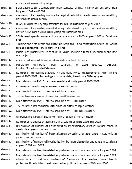
Figure 2.1. Theoretical Variogram parameters. Range (a), Sill (C) and Nugget (C0)
The characteristic parameters of a variogram are:
Sill (C): The semivariance value at which the variogram levels off. Also used to refer to the “amplitude” of a certain component of the semivariogram.
Range (a): The lag distance at which the semivariogram (or semivariogram component) reaches the sill value. Presumably, autocorrelation is essentially zero beyond the range.
Nugget (C0): In theory the semivariogram value at the origin (0 lag) should be zero. If it is
significantly different from zero for lags very close to zero, then this semivariogram value is referred to as the nugget. The nugget represents variability at distances smaller than the typical sample spacing, including measurement error.
The semivariance function is represented by the following equation:
(
)
∑
=
+ −
= N (h)
1 i
2 i i
P
P
) h X ( Z ) x ( Z )
h ( N 2
1 )
h (
γ (2.2)
NP(h): total pair numbers at distance h; h: distance between pairs
Z(xi): experimental values at each location xi xi: spatial locations
• Spherical model: > ≤ − = a h C a h a h 2 1 a h 2 3 C ) h ( 3 γ (2.3)
• Exponential model:
− − = a h exp 1 C ) h ( γ
|h| > 0
(2.4)
• Gaussian model:
− − = 2 2 a h exp 1 C ) h ( γ
|h| > 0
(2.5)
The spherical model actually reaches the specified sill value, C, at the specified range, a.
The exponential and Gaussian approach the sill asymptotically, with a representing the practical range, the distance at which the semivariance reaches 95% of the sill value. The Gaussian model, with its parabolic behavior at the origin, represents very smoothly varying properties. (However, using the Gaussian model alone without a nugget effect can lead to numerical instabilities in the kriging process). The spherical and exponential models exhibit linear behavior the origin, appropriate for representing properties with a higher level of short-range variability.
Figure 2.2. Theoretical variogram models (Spherical, Gaussian and Exponential)
Ordinary Kriging (OK) is a variety of kriging which assumes that local means are not necessarily closely related to the population mean, and which therefore uses only the samples in the local neighborhood for the estimate. Equations 2.6 to 2.8 present OK mathematical definition.
∑
= Z(x ) )
v (
Z* λi i (2.6)
∑
λiγ(xi,xj)+µ=γ(xj,µ) (2.7)∑
− += λγ γ µ
σ2 i (xi,v) (v,v) (2.8)
v: spatial location for prediction Z*(v): estimated value by kriging µ: sample mean
σ2
: estimation variance λi: kriging weights
Simple kriging(SK) uses the average of the entire data set, while ordinary kriging uses a local average (the average of the scatter points in the kriging subset for a particular interpolation point). As a result, simple kriging can be less accurate than ordinary kriging, but it generally produces a result that is "smoother" and more esthetically pleasing.
Block Krigingestimates the value of a block from a set of nearby sample values using kriging.
Spherical
Gaussian
Point Krigingestimates the value of a point from a set of nearby sample values using kriging. The kriged estimate for a point will usually be quite similar to the kriged estimate for a relatively small block centered on the point, but the computed kriging standard deviation will be higher. When a kriged point happens to coincide with a sample location, the kriged estimate will equal the sample value.
Universal Kriging (UK) is a procedure similar to that of punctual kriging, but used when a trend, or slow change in average values, in the samples exists.
Indicator kriging (IK) is a geostatistical approach to geospatial modeling. Like OK, the correlation between data points determines model values. However, IK makes no assumption of normality and is essentially a non-parametric counterpart to OK. Instead of assuming a normal distribution at each estimate location, IK builds the cumulative distribution function (CDF) at each point based on the behavior and correlation structure of indicator transformed data points in the neighborhood (Lloyd and Atkinson, 2001). To achieve this, IK needs a series of threshold values between the smallest and largest data values in the set. These threshold values, referred to here as IK cutoffs, are used to numerically build the CDF of the estimation point. For each IK cutoff, data in the neighborhood are transformed into 0s and 1s: 0s if the data are greater than the threshold, and 1s if they are less. IK then estimates the probability that the estimation point is less than the threshold value, given this neighborhood of transformed data and a model of the IK cutoff correlation structure. Performing this operation for each cutoff across the range of data approximates the CDF at the estimation point. After the CDF is built, it must be post processed to produce probability maps for estimation maps and risk maps.
2.3.2 Bayesian maximum entropy
The Bayesian Maximum Entropy (BME) method has been successfully used in the mapping analysis of environmental contaminants in groundwater, surface water and ambient air (Vyas and Christakos, 1997; Christakos and Serre, 2000; Serre and Christakos, 2004). BME is based on modern spatio-temporal geostatistics (Christakos, 2000), so that classical geostatistics is a specific case of the former. There are several coordinate systems that can be used in BME compared with the Euclidean system on which ‘classical’ geostatistics is based. In this chapter a brief review of BME general principle is presented.
2.3.2.1 Spatio-temporal random field representation
In these studies a space/time random field (S/TRF) Z(p) is used to represent the
The total physical knowledge (K) available regarding a pollutant distribution is assumed to be composed by two main knowledge sources covering both, the general (G) and case-specific (S) knowledge, so that:
K= G ∪ S (2.9)
The G refers to background knowledge that includes physical laws, structured patterns and assumptions, and statistical moments. Some examples of G base are given in Table 2.3.
Table 2.3. Examples of general knowledge G bases Gα
Covariance
(
)(
)
j j i
i x x x
x − −
Variogram
(
)
22 1
j
i x
x −
λ-th order moment (ݔ− ݔതതതതప)
λ
λ=1, …, L
The S refers to specific situation of the study case, includes empirical observations,
site-specific data, etc. As a matter of fact, forPM10 mapping purposes, the specific knowledge
base, S, will denote physical data ,xdata, obtained at points pi(i=1, …, m) for specific X, Y
location coordinates. The S base is formed by two main contributions:
S: ݔௗ௧ = (ݔௗ, ݔ௦௧) (2.10)
Hard data are exact measurements of pollutant concentrations. In contrast, soft data may
include uncertain evidence about the random vector, xsoft. The xsoftcould be expressed in
terms of intervals or in a probabilistic form (Christakos and Serre, 2000).
2.3.2.2 Bayesian maximum entropy estimates
The integration and processing of the physical knowledge based on K leads to the
posterior BME probabilistic density function (PDF) fk(xk)which, in turn, provides the full
stochastic description of pollutant concentration (PM10) at any estimation point pk of
interest. The BME posterior PDF fk(xk) can be expressed as (Christakos and Serre, 2000),
) x , x , x ( f ) x ( f dx A ) x (
fk k = −1
∫
soft S soft G hard soft k (2.11)Where xhard,xsoft, xkrepresent the S/TRF for the pollutant at the hard, soft and estimation
points, respectively, fS(xsoft) is a PDFdescribing the uncertainty for the pollutant at the soft
data points, fG(xhard, xsoft,xk) is a PDF integrating general knowledge about the pollutant
and A is a normalization constant. From the posterior PDFfk(xk) we can obtain several
estimators of the pollutant concentration at the estimation point pk. BME allows the
flexibility to choose among several estimators, and the choice of the best suited estimate will depend on the individual characteristics of each mapping situation. A common
estimator used in environmental mapping analysis is the BME median estimator,xk,median,
defined as the 50% quantile of the BME posterior PDF, and given by the following equation:
∫
∞ − = mean , k xˆ k k kkx f (x ) .
dx 05 (2.12)
Furthermore, because of the inherent randomness of the pollutant transport processes in air and the physical data inaccuracies, it is essential to assess the uncertainty associated with the estimated values (Christakos and Serre, 2000; Christakos et al., 2002)
The variance of the BME posterior PDF provides a useful assessment of the estimation
accuracy for the BME median estimator. The BME posterior variance is denoted by σ2k/k
and is given by:
) x ( f ) x x (
dxk k k,mean k k k
k
2
2 = −−
σ (2.13)
This quality measure corresponds to the variance of the estimation error. However, unlike the classical kriging variance that is independent of the data values (the kriging variance is only covariance and spatial data configuration dependent, must not be confused with the
variance of the kriging predictor), the σ2k/k depends on the specific set of data values
2.4 Artificial neural networks
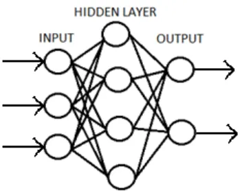
Artificial Neural Networks (ANN) are mathematical models inspired by the structure and functionality of biological neural networks (Hagan, et. al., 1996). A neural network consists of a number of simple processing units called neurons. Each neuron is connected to others by a weightedlink (wij in Figure 2.3).
Figure 2.3. Simple neuron model in an ANN
ANN can be thought of as a model which approximates a function of multiple continuous inputs and outputs. The network consists of a topology graph of neurons (Figure 2.3), each of which computes a function (called an activation or transfer function, f) of the inputs carried on the in-edges and sends the output on its out-edges. Principal activation functions are summarized in Table 2.4. The inputs and outputs are weighed by weights (wij) and shifted by bias factor (bi) specific to each neuron. The bias is an activation
threshold that allows shifting of the activation function to the left or to the right.
The output of a neuron is computed by the following equation:
ܱ = ݂ ൭ ݓݔ+ ܾ
ୀଵ
൱ (2.14)
Oi is the output of the jth neuron, f is the activation or transfer function of the neuron, bj
is the bias of jth neuron, wij is the synaptic weight corresponding to the ith synapse of jth
neuron, xi is the ith input signal to jth neuron and n is the number of input signals to the jth neuron.
Table 2.4. Activations functions used in ANN
Name Formula
Identity ݂(ݔ) = ݔ
Sigmoid ݂(ݔ) = 1
1 + ݁ି௫
Tanh ݂(ݔ) =݁
௫− ݁ି௫
݁௫+ ݁ି௫
Step ݂(ݔ) = ൜−1 ݂݅ ݔ < 0
1 ݂݅ ݔ ≥ 0
Different algorithms of “learning” defines different types of ANN, the principals are:
• Feed-forward neural networks (FFN)
• Radial basis function networks (RBFN)
• Self-organizing maps (SOM)
• Recurrent neural networks (RNN)
• Fuzzy ARTMAP Networks
2.4.1 Feed-forward neural networks
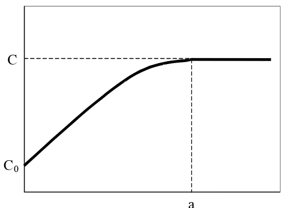
A feedforward neural network is an artificial neural network where the information moves only in one direction, from input to output nodes without any cycle or loop in the network.
Figure 2.4.Multilayer perceptron feed-forward neural network architecture
of the network (weights and biases) are updated (updating step). In the training phase the error in the output node j in the nth data point is represented by
݁ = ݀(݊) − ݕ(݊) (2.15)
Where d is the target value and y is the value produced by the neuron. Corrections to the
weights of the neurons are made based on minimization of the error in the entire output layer (equation 2.16). Minimization by gradient descent gives the change at each weight
(equation 2.17) where yi is the output of the previous neuron and α is the learning rate,
which is selected to ensure fast and non-oscillatory convergence of the weights (typically ranges between 0.2 to 0.8). The errors propagate backwards from the output nodes to the inner nodes, and this can be accomplished by two methods: on-line learning and batch learning. In on-line learning, the updates of weightsare performed at each propagation stepand requiresmore updates than the batch algorithm. In batch learning the updating of weights is performed after a certain number of propagation stepsand requires more memory capacity than the previous one. Some limitations of backpropagation learning algorithm are that convergence is not guaranteed and (if existing) is very slow, also local minima can be found and normalization of input is required.
ߝ(݊) =12 ݁ଶ(݊)
(2.16)
∆ݓ(݊) = −ߙ߲ݒ߲ߝ(݊)
(݊) ݕ(݊) (2.17) 2.4.2 Radial basisfunction networks
A radial basis function network (RBFN) is a two-layer ANN that uses radial basis functions as activation functions in its hidden layer, and linear functions in its output layer (Lo, 1998). Types of radial basis functions are summarized in Table 2.5. Gaussian bell functions are the most used activation function in RBFN. Most applications of RBFN are in the field of function approximation, time series prediction and process control.
Table 2.5. Radial basis functions
Name Formula
Gaussian ݂(ݔ) = ݁ି(ఌ)మ
Multiquadric ݂(ݔ) = ඥ1 + (ߝݎ)ଶ
Inverse quadratic ݂(ݔ) = 1
1 + (ߝݎ)ଶ
Inverse
Multiquadric ݂(ݔ) =