Elliptic and parabolic PDEs : regularity for nonlocal diffusion equations and two isoperimetric problems

(1)

Universitat Polit`

ecnica de Catalunya

Programa de Doctorat de Matem`

atica Aplicada

Departament de Matem`

atica Aplicada I

Elliptic and parabolic PDEs:

regularity for nonlocal diffusion equations

and two isoperimetric problems

by

Joaquim Serra

PhD dissertation

(2)

(3)

Acknowledgments

I am greatly indebted to Xavier Cabr´e, who has been the optimal advisor during these years. Most mathematics that I know, I have learnt from him. Furthermore, he has constantly encouraged me and he has been always available. I appreciate very much his extraordinary dedication.

My friend Xavier Ros, with whom I have been very lucky to share Cabr´e as advisor, has also helped me a lot. I have enjoyed and learnt much when discussing mathematics (and sometimes politics) with him.

I am thankful to Josep Gran´e, who was not only the responsible of me deciding to study mathematics, but who also sent me later to Cabr´e. His encouragement and directions during more than ten years —since I went for the first time to one of his open lectures for the mathematical olympiad— have been crucial to my career.

Other very important people in my relationship with mathematics have been my friends Miguel Teixid´o and Elisa Lorenzo, and my professor in Batxillerat, Mariona Petit. I am also indebted to them.

Last, but not least, I own very much to my partner, Neus, little Max, my parents, and remaining family. Their unconditional support and help during these years have been extremely important to me.

(4)

(5)

Summary

This thesis is divided into two parts.

The first part is mainly concerned with regularity issues for integro-differential

or nonlocal equations. The elliptic integro-differential operatorsL of the form Lu(x) =

Z

Rn

u(x+y) +u(x−y)

2 −u(x)

b(y)

|y|n+2sdy with 0< λ≤b(y)≤Λ (0.1) are infinitesimal generators of L´evy processes. Thus, in the same way that densities of particles with Brownian motion solve second order elliptic or parabolic equations, the equations Lu = 0 or ut = Lu are satisfied by densities of particles with L´evy motion.

Whenb(y) is constant, the operatorLis the fractional Laplacian−(−∆)s_{, which} can be also defined via Fourier transform as F (−∆)s_u

=|ξ|2s_F_(u).

The well-posed Dirichlet problem for these operators is a problem with comple-ment data:

(

Lu=f in Ω

u= 0 in_Rn_\_Ω. (0.2)

There are many classical regularity results for (−∆)s _{—whose “inverse” is the} Riesz potential. For instance, the explicit Poisson kernel for a ball is an “old” result, as well as the Lp _{solvability of the equation (−∆)}s_u₌_f _{in the whole}

Rn. However, very little was known on boundary regularityfor problems of the type (0.2). A main topic of this thesis is the study of this boundary regularity, which is qualitatively different from that for second order equations.

Our first result in this direction is for problem (0.2) with L=−(−∆)s_{. In this} case we prove that solutions u are Cs up to the boundary and, more importantly, that the quotient u/ds ∈ Cα(Ω), for some small α > 0, where d is the distance to the boundary ∂Ω. Note that the solution to (−∆)s_u _{= 1 in} _B

1, u ≡ 0 outside B1 is given by the explicit expression u(x) =c(1− |x|2)s+, where c is some positive constant. Hence, the regularity u∈Cs _{cannot be improved. Instead, finer boundary} regularity for these fractional order equations means higher order H¨older regularity of u/ds_.

The previous estimates for (−∆)s _{are crucial to establish the Pohozaev identity} for the fractional Laplacian, a main result of this thesis. This new identity applies

(6)

4 SUMMARY

to solutions of (−∆)s_u₌_{f(u, x) in Ω,} _u_{= 0 in}

Rn\Ω, and reads as follows Z

Ω

(x· ∇u)(−∆)s_{u dx}₌ 2s−n 2

Z Ω

u(−∆)s_{u dx}₋ Γ(1 +s)2 2

Z ∂Ω

u ds

2

(x·ν)dσ. This identity does not follow from some “vector calculus identity” and the divergence theorem, as it is the case in the classical Pohozaev identity. Instead, its proof is more delicate mainly due to the more intricate boundary behavior of solutions.

Our methods to prove H¨older regularity foru/ds_{are based only on the maximum} principle, the Harnack inequality, and on suitable barriers (we develop a nonlocal version of the Krylov method for second order elliptic equations with bounded mea-surable coefficients). This allows us to obtain results also for fully nonlinear integro-differential equations, arising in stochastic integro-differential games. Our results apply to fully nonlinear equations with respect to the class L∗, containing all operators L of the form (0.1) which arescale invariant, i.e. b(y) =a(y/|y|). This class is comprised by infinitesimal generators of 2s-stable L´evy processes. We prove that solutionsuto (0.2) where L is replaced by a fully nonlinear operator (such as infβsupαLαβ with Lαβ ∈ L∗), satisfy u/ds ∈Cβ(Ω) for all β ∈(0, s). In addition, we show counterex-amples to this boundary regularity in the larger ellipticity class L0 of Caffarelli and Silvestre, which contains alloperators of the form (0.1).

We also obtain new interior regularity results for fully nonlinear nonlocal par-abolic equations with rough kernels in the class L0. We prove that solutions to these equations with merely bounded complement data are Cβ _{in space and}_C₂β_s _in time for all β < {2s,1 +α}, where α > 0. These results are nearly optimal. For it, we develop a new regularity method for nonlocal equations based on a Liouville theorem and a blow up and compactness argument. It allows to avoid a recurrent difficulty in integro-differential equations when trying to iterate nonlocal estimates We believe that this method, which is very flexible and solves the previous difficulty, is a main contribution of the thesis. For instance its use has been essential to prove our boundary regularity results for fully nonlinear equations, described above.

In this first part of the thesis we have also studied semilinear equations with nonlocal diffusion operators. On the one hand, by finding an extension problem for a sum of fractional Laplacians, we are able to prove 1-D symmetry of phase transitions in dimensionn= 2 for equations of the typeP

i(−∆)

si_u₊_W0_{(u) = 0 in} Rn, whereW is a double well potential and si ∈(0,1). We also obtain symmetry in dimension n= 3 provided minsi ≥1/2. One the other hand, we study the nonlocal version of the extremal solution problem (−∆)s_u ₌ _λf_{(u) in Ω. For this problem} we obtain some initial results on boundedness of the extremal solution extending well-known and important ones for s= 1. In addition, and as an application of our Pohozaev identity, we prove that the extremal solution belongs to Hs.

(7)

SUMMARY 5

cones with densities. We show that given a convex cone Σ ⊂ _Rn _{and a weight} w ∈ C(Σ) which is homogeneous of degree α >0 and such that w1/α _{is concave in} Σ, the isoperimteric quotient

R

∂Ω∩Σw dσ

1/(n+α−1)

R

Ω∩Σw dx

1/(n+α)

is minimized by balls centered at the origen. We also obtain an anisotropic version of this result. This is done by generalizing a proof of the classical isoperimetric inequality due to X. Cabr´e. Our new results contain as particular cases the classical Wulff inequality and the isoperimetric inequality in cones of Lions and Pacella.

In the second instance we use the isoperimetric inequality and the classical Po-hozaev identity to establish a radial symmetry result for second order reaction-diffusion equations. The novelty here is to include discontinuous nonlinearities. For this, we extend a two-dimensional argument of P.-L. Lions from 1981 to obtain now results in higher dimensions.

The thesis is made up of the following articles:

A. X. Ros-Oton, J. Serra, The Pohozaev identity for the fractional Laplacian, to appear in Arch. Rational Mech. Anal.

B. X. Ros-Oton, J. Serra, The Dirichlet problem for the fractional Laplacian: regularity up to the boundary, J. Math. Pures Appl. 101 (2014), 275-302. C. X. Ros-Oton, J. Serra,Nonexistence results for nonlocal equations with

crit-ical and supercritcrit-ical nonlinearities, preprint ArXiv (2013).

D. J. Serra, Regularity for fully nonlinear nonlocal parabolic equation with rough kernels; preprint ArXiv (2014).

E. X. Ros-Oton, J. Serra, Boundary regularity for fully nonlinear integro-differential equations, preprint Arxiv (2014).

F. X. Ros-Oton, J. Serra, The extremal solution for the fractional Laplacian, Calc. Var. Partial Differential Equations, published online.

G. X. Cabr´e, J. Serra,An extension problem for sums of fractional Laplacians and 1-D symmetry of phase transitions, preprint (2013).

H. X. Cabr´e, X. Ros-Oton, J. Serra, Sharp isoperimetric inequalities via the ABP method, preprint ArXiv (2013).

(8)

(9)

Introduction

The contents of this thesis are divided into two parts. The first, and main one, concerns nonlocal —or fractional— diffusion equations, an extension of standard Brownian diffusion and of the heat equation. The second part includes two instances of interaction between isoperimetryand Partial Differential Equations.

In the first part we study fractional semilinear problems, as well as nonlocal fully nonlinear diffusion equations —both in their parabolic and elliptic versions. We obtain results on interior and boundary regularity for these equations. The boundary regularity results for equations of fractional order are a main novelty of the thesis. They are qualitatively different from their classical versions for second order elliptic equations. In addition, they play an important role in the Pohozaev identity for the fractional Laplacian, which is another central result of the thesis. In this first part we also study a nonlocal phase transition problem, as well as the fractional version the semilinear extremal solution problem.

This first part of the thesis iscomprised of the following articles:

[A] X. Ros-Oton, J. Serra,The Pohozaev identity for the fractional Laplacian, to appear in Arch. Rational Mech. Anal.

[B] X. Ros-Oton, J. Serra,The Dirichlet problem for the fractional Laplacian: regularity up to the boundary, J. Math. Pures Appl. 101 (2014), 275-302.

[C] X. Ros-Oton, J. Serra,Nonexistence results for nonlocal equations with critical and supercritical nonlinearities, preprint ArXiv (2013).

[D] J. Serra,Regularity for fully nonlinear nonlocal parabolic equation with rough kernels; preprint ArXiv (2014).

[E] X. Ros-Oton, J. Serra, Boundary regularity for fully nonlinear integro-differential equations, preprint Arxiv (2014).

[F] X. Ros-Oton, J.Serra, The extremal solution for the fractional Laplacian, Calc. Var. Partial Differential Equations, published online.

[G] X. Cabr´e, J. Serra,An extension problem for sums of fractional Laplacians and 1-D symmetry of phase transitions, preprint (2013).

In the second part we include two instances of interaction between isoperimetric inequalities and elliptic PDE. In the first one we use the Alexandrov-Bakelman-Pucci method for elliptic PDE to obtain new sharp isoperimetric inequalities in cones with densities. This is done by generalizing a proof of the classical isoperimetric inequality due to X. Cabr´e. Our new result contains as particular cases the classical

(12)

10 INTRODUCTION

Wulff inequality and the isoperimetric inequality in cones of Lions and Pacella. In the second instance the interaction goes on the opposite direction: we use the isoperimetric inequality and the classical Pohozaev identity to establish a radial symmetry result for second order reaction-diffusion equations. The novelty here is to include discontinuous nonlinearities. For this, we extend a two-dimensional argument of P.-L. Lions from 1981 to obtain now results in higher dimensions.

This second part of the thesis is comprised of the following two articles:

[H] X. Cabr´e, X. Ros-Oton, J. Serra,Sharp isoperimetric inequalities via the ABP method, preprint ArXiv (2013).

[I] J. Serra, Radial symmetry for diffusion equations with discontinuous nonlinearities, J. Differ-ential Equations 254 (2013), 1893-1902.

The introduction is divided into two sections, corresponding to the division ex-plained above.

(13)

1. Nonlocal diffusions

1.1. From Brownian to L´evy models. In mathematics, and more particu-larly in PDE, the (main) equation to model diffusion is the heat equation

ut−∆u= 0. (1.1)

It is a well-known fact that the probability distribution function (which depends on time) for a Brownian motion satisfies (1.1). By this reason, a wide variety of physical phenomena are modeled by the heat equation. A short list of typical examples includes: diffusion of a pollutant in the air, bacterial diffusion, disease propagation, error propagation in numerical analysis, or stock market prices.

Let us develop in more detail the example of the stock prices. This example turns out to be very appropriate to motivate the results of this thesis, and it will appear again in this introduction. Let

X(t) = X1(t), . . . , Xn(t)

be a vector with the share prices of n different corporations at time t. The Brow-nian model for share prices, also known as Merton-Samuelson model, describes the fluctuation of the logarithmic prices as a n-dimensional Brownian motion. Namely, letting

Yi = log(Xi),

the model states (in the language of stochastic differential equations) that dYi =µidt+

d X k=1

σikdWk. (1.2)

Here, µiare the drift coefficients,σik are the (joint) volatilities, andWkare indepen-dent Wiener processes, also called Brownian processes. Actually, (1.2) corresponds to the simplest version of the model, in which drifts and volatilities are taken con-stant in time.

For all modeling purposes, after discretizing time by choosing a small time step τ > 0, the previous stochastic differential equation can be understood as the follow-ing recursive relation

Yi(t+τ)−Yi(t) =µiτ + d X

k=1 σik

√

τ ξk(t), (1.3)

where t∈τ_Z and ξk(t) are noise variables that have Gaussian distributionN(0,1), with zero mean and unit variance. The drandom variables ξk(t) are assumed to be independent of each other and also independent of their past values {ξk(s), s < t}. It is of course important the square root √τ, appearing in (1.3) in front of the noise variables ξj(t). If

√

τ was replaced by a smaller factor (say τ orτ2/3_{), then in} the limitτ &0 we would obtain a deterministic model; the stochastic part would be

killed by the too small factor. This is clearly related to the Central Limit Theorem:

(14)

12 INTRODUCTION

the sum of a large number N of independent random variables divided by √N (and not N nor N2/3_{) converges to a Gaussian law} _N_(0,_1).

If u(x, t) is the probability density function of Y(t) then, when µi = 0, we have ut−

n X i,j=1

aij∂iju= 0 in Rn, for aij = P

k 1

2σikσjk. This equation gives the (a priori unclear) link between the fluctuation of market prices and heat conduction. This connection also makes the model (1.2) to enjoy nice mathematical properties.

Although the model (1.2) is quite simple (contains few parameters), it is known to be quite accurate. Other than the drift parameters µi, which quantify long-term trends of prices, this model depends only on a matrix of parameters σij, the volatilizes. Until the last decades, simplicity was a very important advantage of this (and every) model. Indeed, the values of the parameters need to be calibrated by

fittingthe model to the existing market data —for instance by a maximum likelihood criterion. A small number of parameters is crucial when data is (or was) scarce since, otherwise, the model will easily overfit1.

However, the available amount of market data increases extremely fast, and so does computational power. For instance, it is nowadays easy to download gigabytes of historical market data in few minutes and to fit quite involved models to it using a regular laptop. Thus, it seems no longer necessary in applications to consider so simple models, but rather it may be an oversimplification in some situations. Still, the mathematical simplicity of a model will always be a virtue and allows to understand the crucial issues of a problem.

From the more theoretical point of view, there are some well-known inconsisten-cies of the model (1.2) like the implied volatility smile. This is a famous paradox

to the Black-Scholes theory for option pricing, and it is usually attributed to the inaccuracy of (1.2) —a main assumption of the Black-Scholes theory. At the same time, a reasonable criticism to the Brownian model is that, according to it, stock market prices should be scale invariant (since Brownian motion is). But they are not Ideed, it is known that the behavior of stock market prices is typically different in middle and large times scales —with the Brownian model being more accurate in larger time scales, due to the Central Limit Theorem.

It is thus not surprising that, since the seventies, many authors have considered more general models in which (1.2) is replaced by the natural assumption that Y(t) is a Lévy process —see for instance [91, 48, 88, 96] and references therein. As explained in the next section, Lévy processes are Stochastic processes with no mem-ory and stationary increments. These properties make Lévy processes the rational model of noise or random perturbations. Brownian motion is a distinguished par-ticular case in this large class of processes. From the mathematical point of view, 1_{Like if we use a polynomial of degree 99 to fit a cloud of 100 points which are rather aligned:}

(15)

1. NONLOCAL DIFFUSIONS 13

Brownian motion is the only L´evy process with continuous sample paths. However, in real world data, time is always discrete —as in (1.3)— and hence continuity of sample paths is only an ideal property which is impossible to see or test. What we do see is whether time increments are stationary and also the absence of memory, and these two properties are shared by allL´evy processes.

Although this discussion was focussed in mathematical models of the financial market, it is clear that the same issues (need of more accuracy, known inconsis-tencies, increasing amount of data, discrete time models) apply to many diffusive models in science where the Brownian diffusion has also been replaced by a L´evy one. For instance, this seems specifically relevant in models of population dynamics in biology and social sciences [79, 100, 123].

In the next section we introduce L´evy processes and some of their main proper-ties.

1.2. L´evy processes. A n-dimensional L´evy process is a stochastic process taking values in _Rn _{and that has stationary and independent increments. It is also} assumed to satisfy Y(0) = 0 and to be continuous in probability, i.e., given t > 0, the probability thatY(t+h)−Y(t)

> tends to zero ash&0 for all >0 and for a.e. t. This does notmean that the sample paths of a L´evy process are continuous, and in fact they are not —with the sole exception of Brownian motion. That Y(t) has independent, stationary increments means that the law of Y(t +h)− Y(t) depends only on h (not on t), and that Y(t+h)−Y(t) is independent of the past {Y(s), s < t}.

While (1.2) depends only of a finite number of real parameters (µi and σij), a L´evy process depends on the choice of a measure µ in _Rn \ {0} satisfying the condition

Z

Rn\{0}

1∧ |y|2dµ(y)<∞, (1.4)

where∧denotes the minimum. Measuresµsatisfying (1.4) are calledL´evy measures. If Y(t) is a L´evy process, we define its infinitesimal generator L as the linear translation invariant operator that acts on functions u∈C_c∞(_Rn) as follows:

Lu(x) = lim t&0

Eu x+Y(t)−u(x)

t . (1.5)

As a consequence of the L´evy-Khintchine representation formula [8], the infinitesimal generators of L´evy processes are exactly the operators of the form

Lu(x) = aij∂iju(x)+bi∂iu(x)+ Z

Rn\{0}

u(x+y)−u(x)−∇u(x)·yχB1(x) µ(dy), (1.6)

(16)

14 INTRODUCTION

General references for L´evy processes are [2, 8].

The adjoint operator Ladj _{of the infinitesimal generator} _L _{carries all the} infor-mation on the law ofY(t). Namely, ifp(x, t) denotes the probability distribution of a n-dimensional L´evy process Y(t), defined by

Z A

p(x, t)dx=_P(Y(t)∈A) for all A, then p(x, t) solves the evolution equation

pt=Ladjp inRn. (1.7)

That the adjoint operator Ladj _{(and not} _{L) must appear in (1.7) also happens for} second order operators aij(x)∂ij and ∂ij aij(x)·

, and their relation with Markov processes. Namely, if a n-dimensional Markov process Z(t) solves

(

dZi(t) = P

kσik Z(t)

dWk(t),

Z(0) =x0.

then the probabilitydensityfunctionp(x, t) ofZ(t) satisfies the Fokker-Planck equa-tion

pt =∂ij aij(x)p, where aij(x) = 1₂

P

kσik(x)σjk(x). Instead, the operator aij(x)∂ij appears in the Kolomogorov equation, which is satisfied byexpectationtype quantities likeu(x0, t) = Eϕ Zx0(t)

, where ϕ ∈ C_c∞(_Rn_{). Similarly, expectation type quantities for L´}_evy processes are often described by equations involvingLinstead ofLadj, as seen in the following example.

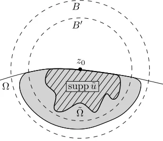
Example 1.1. Let Y(t) be a L´evy process, Ω be a bounded domain and let ϕ∈C_c∞(_Rn_\_{Ω). Given} _x

0 ∈Ω let

u(x0) = Eϕ x0+Y(Tx0)

,

where Tx0 is the first time at with the process x0+Y leaves Ω, that is

Tx0 = inf

t >0 : x0+Y(t)

/ ∈Ω .

Note that Tx0 is a random variable (a so called stopping time). Note also that

u(x0) =Eu x0+Y(t∧ Tx0)

for all t >0. Thus, (at least formally) we have

0 = lim t&0

Eu x0+Y(t∧ Tx0)

−u(x0)

t =Lu(x0) for all x0 ∈Ω. It follows that u is a solution of the nonlocal problem

(

(17)

where L, as in (1.5) and (1.6), is the infinitesimal generator of Y(t). Although this argument is formal, it can be made rigorous if the previous equation has good regularity estimates.

1.3. Nonlocal elliptic operators. Key differences with the second or-der case. The infinitesimal generators of L´evy processes are linear elliptic integro-differential operators. They are typically nonlocal, meaning that the value of Lϕ at a point x0 ∈_Rn_{, given by (1.6), depends on the values of} _ϕ_{outside a neighborhood} of x0. When µ >0 in Rn\ {0}, Lϕ(x0) depends on the values of ϕat all points of Rn. This is a clear contrast with local second order operators, which can be eval-uated at one point only knowing the values of the function in an arbitrarily small neighborhood.

Let us explain next in what senseLiselliptic. Assume thatϕ∈C2₍

Rn)∩L∞(Rn) has a global minimum at x0 ∈Rn. Then, either using (1.5) or (1.6) we obtain

Lϕ(x0)≥0.

This property of the operator being nonnegative at points of minimum is the vis-cosity notion of ellipticity.

However, let us point out two important differences with second order elliptic operators. Again consider µ >0 in _Rn_{\ {0}. We then have:}

(a) Thatϕ≥ϕ(x0) in a neighborhood ofx0 is not enough to ensureLϕ(x0)≥0. Instead, we must require ϕ≥ϕ(x0) in all of Rn.

(b) Ifϕ≥ϕ(x0) in all of Rn then either Lϕ(x0)>0 orϕ≡ϕ(x0) in all ofRn. Both (a) and (b) follow easily from the definition of L in (1.6) when µ > 0. While (a) is a “disadvantage” with respect to second order local operators, (b) is a very favorable counterpart. Note that (b) has the flavor of a strong maximum princi-ple but, in a dramatic contrast with second order operators, the sole information Lϕ(x0) = 0 at the point of minimumx0 is enough to conclude that ϕis constant in all of _Rn_!

The two key differences (a) and (b) of nonlocal elliptic operators with respect to local ones appear repeatedly in the regularity theory of elliptic and parabolic integro-differential equations. The global nature of the maximum principle in (a) causes difficulties and forces to control the solutions in the whole_Rn—estimates are nonlocal, Harnack inequality is only available for solutions which are nonnegative in the whole _Rn_{, etc. Instead, property (b) makes some things easier than for} local equations. A good example of this is the quick proof of Luis Silvestre [110] of the H¨older regularity for nonlocal elliptic equations with “bounded measurable coefficients”. Another example is the proof of the Bernstein theorem for nonlocal minimal surfaces of Figalli and Valdinoci [68].

(18)

16 INTRODUCTION

−(−∆)s_{, where} _s_∈_(0,_{1). It is equivalently defined either by the integral} −(−∆)s_{u(x) =}_c

n,s Z

Rn

u(x+y) +u(x−y)

2 −u(x)

1

|y|n+2sdy (1.8) or via Fourier transform as

F

(−∆)s

(ξ) =|ξ|2s_F[u](ξ). _(1.9)

As a consequence of (1.9) we have (−∆)s_◦_(−∆)t_{= (−∆)}s+t_{, which motivates the} name fractional Laplacian.

The fractional Laplacian is the only nonlocal elliptic operator which is transla-tion, rotatransla-tion, and scale invariant. In this sense, it is similar to the ∆. However, note the following important difference between the cases s = 1 and s < 1. While every linear translation invariant elliptic operator of order 2 is the Laplacian after some affine change of coordinates, for s <1 there are many more linear translation invariant operators of order 2s than just affine transformations of (−∆)s _—for in-stance all the infinitesimal generators of 2s-stable L´evy processes of the form (1.21). Thus, zoology of operators in the nonlocal setting is richer than in the second order case.

1.4. Nonlinear analysis for nonlocal operators: mathematical back-ground. The study of linear integro-differential elliptic equations was initiated by the Probability community in the 1950’s —not surprisingly given the strong proba-bilistic motivation of these equations. Many authors, like Blumenthal, Getoor, Kac, or more recently Bogdan, Bass, and Kassmann (to name only a few) have made important contributions using mostly probabilistic techniques. In parallel to this, the potential theory for the fractional Laplacian (Riesz potentials) was studied in detail, starting by Riesz [101] himself, and there are even classical references on the topic like the book of Landkov [85]. For instance, the explicit Poisson kernel in a ball for the fractional Dirichlet problem (−∆)us ₌ _f _in _B

1, u = g in Rn\B1 is a classical result [81, 74]. These early results for nonlocal equations concerned mainly linear equations.

It has not been until the last decade, coinciding with the irruption of nonlocal equations in the PDE community, that nonlinearintegro-differential equations have been studied in depth. Some fractional nonlinear problems (with many relations existing among them) that have been studied in the last years include:

• Reactions on the boundary; layer solutions to nonlocal reaction-diffusion equations; De Giorgi type conjecture; nonlocal fractional perimeters; non-local minimal surfaces.

• Fractional obstacle problem; one phase problem.

• Fully nonlinear elliptic and parabolic integro-differential equations; pertur-bative methods for these equations.

(19)

• Nonlinear diffusions; front propagation; fractional versions of the porous media equation.

• Fractional semilinear problems; existence, symmetry, and qualitative prop-erties, uniqueness of ground states.

• Fractional equations and curvatures from conformal geometry.

In the remarkable paper [3] from 1991, Amick and Toland found all solutions in _R to the Benjamin-Ono equation (−∆)1/2_u ₌ _−u₊_u2_{. As already observed by} Benjamin, the previous equation is equivalent to

(

∆v = 0 in _R2

+

∂νv =−v+v2 on ∂R2+={x2 = 0},

(1.10) This fact is crucially used in the analysis of [3]. Later, Toland [118] classified the solutions to the Peierls-Nabarro equation (−∆)1/2_u _{= sin(πu) in}

R by unraveling an intrinsic link of this equation with the Benjamin-Ono equation.

For more general nonlinearities, Cabr´e and Sol`a-Morales [27] studied boundary reaction problem

(

∆v = 0 in_Rn+1₊

∂νv =f(v) on∂Rn+1+ ={xn+1 = 0},

(1.11) wherefis a bistable nonlinearity. In [27] some important classical results for interior reactions −∆u=f(u) were proved to hold also for (1.11). Among other results, the authors showed a Modica type estimate in dimension n= 1 and proved the analogue of the De Giorgi conjecture in dimension n = 2.

As in [3, 118], problem (1.11) is equivalent to (−∆)1/2_u ₌ _f_{(u) in}

Rn, where u(x) = v(x,0), x ∈ _Rn_{. Heuristically, the reason why the Dirichlet-to-Neumann} operator T : u 7→ ∂

∂νv, where v is the harmonic extension of u in R n+1

+ , coincides with the half Laplacian (−∆)1/2 _{is the following. If we apply it twice we obtain}

T2u(x) =∂ννv(x,0) =∂xn+1xn+1v(x.0) =−

n X

i=1

∂xixiv(x,0) = (−∆)|Rnu(x). The H¨older regularity for integro-differential elliptic equations “with bounded measurable coefficients”, proved by Bass and Levin [5] and Silvestre [110], opened the door to a regularity theory for fully nonlinear nonlocal elliptic equations, al-though a precise definition of these equations was not given until some year later in [34].

(20)

18 INTRODUCTION

Later, Caffarelli and Silvestre [33] introduced the extension problem tool. Sim-ilarly to what happens for s = 1/2 with the nonlinear problem for (1.11), the extension problem transforms an equation involving (−∆)s _in

Rn with s ∈ (0,1) into a PDE in one more dimension. The new PDE involves the singular elliptic differential operator div (xn+1)1−2s∇ ·) and a Neumann type boundary condition. A remarkable consequence of this new tool is an Almgren type monotonicty formula for solutions to (−∆)s_u_{= 0. This was used by the previous two authors and Salsa} [37] to prove regularity of the solution and of the free boundary for the fractional obstacle problem.

Also using the extension problem, afractional version of the De Giorgi conjecture

was proved in dimension n = 2 for all s ∈ (0,1) and in dimension n = 3 for s ∈ [1/2,1) by Cabr´e and Cinti [20, 21]. Related to this (although not using the extension), Savin and Valdinoci [107, 108] proved a Γ-convergence result (in the spirt of the classical one of Modica and Mortola [92]) for the fractional Allen-Cahn equation. They consider the renormalized energy functional for the rescaled equation (−∆)s_u₌_ε−2s_f_{(u). For} _s_∈_[1/2,_{1] they obtain the Γ-convergence to the} classical perimeter of the renormalized energy functional, as in [92]. Instead, for s ∈ (0,1/2) they obtain Γ-convergence to a fractional perimeter, as introduced by Caffarelli, Roquejoffre, and Savin [31].

An important result which uses the extension problem in an essential way is

uniqueness of ground states for (−∆)s_u₌_−u₊_up _{in dimension 1, proved by Frank} and Lenzmann [70]. Recently, incorporating some ideas of Cabr´e and Sire [28], Frank, Lenzmann, and Silvestre [71] have proved the uniqueness of ground states in every dimension.

(21)

In [4], Barles, Chasseigne, and Imbert studied a different class of fully nonlinear integro-differential equations using methods `a la Jensen-Ishi-Lions. The ideas in [4] are interesting and useful also for the equations considered in [34].

The nonlocal variational theory has also been developed. A main step in this direction was the nonlocal analogue to the De Giorgi-Nash-Moser theory obtained by Kassmann in [84]. Later, motivated by their previous works on the surface quasi-geostrophic equation [38] and on the Navier-Stokes equation [120], Caffarelli, Chan, and Vasseur established the regularity theory for nonlocal parabolic equations in divergence form [30].

Front propagation and nonlinear diffusions have also been studied in the frac-tional context. The exponential speed of invasions has been proved by Cabr´e, Coulon, and Roquejoffre in [22, 23]. Theporous media equation with fractional pres-sure was studied by Caffarelli and V´azquez in [39, 40]. See also [109, 61, 62, 121]. 1.5. Fully nonlinear elliptic and parabolic integro-differential equa-tions: the Stochastic control motivation. Let us consider the following varia-tion of Example 1.1 in secvaria-tion 1.2 in which now a single player controls the law of increments of the process, with the goal of maximizing the expectation of the payoff

received at the first visited point outside Ω.

Example 1.2. Let Y(α;t) be a family of L´evy processes indexed by a control-lable parameter α, and let Lα be the infinitesimal generator of Y(α; ·). A strategy of the player assigns to each x∈Ω some control α[x]. The random motion, stating at x0 ∈Ω, associated to some strategyα[·] is (heuristically)

(

dX(t) = dY α[X(t)];t

X(0) =x0.

Given a bounded payoff function ϕ∈C2(_Rn\Ω), the player wants maximize the expected payoff at the stopping time T = inf{t >0 :X(t)∈/ Ω}. Let us call

u(x0, t) = max

α[·] Eϕ(T). Then, we formally have

u(x0) = lim

t&0maxα u x0+Y(α;t∧ T)

.

FUrthermore, 0 = lim

t&0

maxαu x0+Y(α;t∧ T)

)−u(x0)

t = maxα Lαu(x0).

In Example 1.2 we see that the value (expected payoff) of a single player game (control problem) formally satisfies the equation

maxαLαu = 0 in Ω

(22)

20 INTRODUCTION

In the situation of a zero sum game between two players the equation for the value

of the game is

minβmaxαLαβu = 0 in Ω

u = ϕ in_Rn_\_Ω, (1.13)

where β stands for the possible controls of the second player, whose objective is to minimize the payoff for the first player.

When Lα or Lαβ are restricted to be linear second order elliptic operators, the previous equations are the classical Bellman and Isaacs equations.

Example 1.2 motivates the abstract definition in [34] of fully nonlinear elliptic operator I, explained below, which is the one that we follow.

The equivalent notion in nonlocal equations to the uniform ellipticity for second order equations is ellipticity with respect to some class. The ellipticity class is a given set of linear translation invariant operators, denoted by L, of the form (1.6). The extremal Pucci type operators for a given class L are defined as

M_L+u(x) = sup L∈L

Lu(x) and M_L−u(x) = inf

L∈LLu(x).

Then a fully nonlinear operator I is said to be elliptic with respect to L if the inequalities

ML(u−v)(x)≤Iu(x)−Iv(x)≤ML(u−v)(x)

hold for every pair of test functions u, v atx —i.e.,C2 _{functions in a neighborhood} of x and bounded in the whole space. It is not difficult to see that this definition coincides with the usual definition of second order uniformly elliptic fully nonlinear operator when L={aij∂ij with 0< λId≤(aij)≤ΛId}.

As shown in [34], the “convex” operator Iu= maxαLαuin (1.12) is elliptic with respect to L=S

α{Lα}and Iu= minβmaxαLαu in (1.13) is elliptic with respect to L =S

α,β{Lα,β}.

We say that I is translation invariant when I u(x0 +·)

(x) = (Iu)(x0+x).

Other examples of fully nonlinear translation invariant elliptic operators are those of the form

Iu(x) = inf

α sup_β Lαβu+cαβ

.

As for second order equations, the incremental quotients v of a solutionuto a trans-lation invariant elliptic equation Iu = 0 satisfy the two inequalities M_L+v ≥ 0 and M_L−v ≤ 0. This pair of inequalities is what we sometimes refer as elliptic equa-tion with “bounded measurable coefficients”, even though in the integro-differential context there are no coefficients but kernels.

(23)

smooth function ϕtouches it from above (resp. below) at a point xthen Iϕ(x)≥0 (resp. ≤).

1.6. Results: Pohozaev identity for the fractional Laplacian. A main result of this Thesis is the Pohozaev identity for the fractional Laplacian. For second order equations, the Pohozaev identitity applies to solutions of

−∆u=f(x, u) in Ω, u= 0 on ∂Ω.

The original identity was obtained by Pohozaev [98], who used it to prove the nonexistence of solutions for critical and supercritical nonlinearities f.

There is a collection of identities of Pohozhaev type which have been widely used in the analysis of elliptic PDE. These identities are usually related some to divergence free quantity for the corresponding homogeneous equation. Divergence free quanti-ties are to PDE what conserved quantiquanti-ties are to ODE. They can be found exploiting symmetries of the problem, i.e., using the PDE version of the Noether’s theorem; see [63]. In the original Pohozaev identity (as well as in ours) the underlying symmetry is the scale invariance of the (fractional) Laplacian. Pohozaev identities are used in a several different contexts: monotonicity formulas, unique continuation properties, concentration-compactness results, energy estimates for ground states in _Rn_{, radial} symmetry of solutions, controllability of wave equations, etc.

We have obtained the following fractional version of the Pohozaev identity. It applies to functions that satisfy an equation of the type (−∆)s_u ₌ _{f(x, u), and} u = 0 in _Rn\Ω. These functions u are only Cs(Ω). However, the quotient u/ds, where d is the distance to the boundary, belongs to Cα(Ω), in the sense that the function u/ds_{, defined in Ω admits a continuous extension to Ω. In the last term} of our identity, the quantity u/ds_|

∂Ω is understood as the limit from inside Ω of the function u/ds_.

Theorem 1.3 ([A]). Let Ω be a bounded and C1,1 domain. Assume that u is

a bounded Hs₍

Rn) solution of a semilinear equation of the type (−∆)su = f(x, u),

withf Lipschitz, and u= 0in_Rn_\Ω_{. Then}_u/ds_∈_Cα_(Ω)_{and the following identity}

holds

Z Ω

(x· ∇u)(−∆)s_{u dx} ₌ 2s−n 2

Z Ω

u(−∆)s_{u dx}₋Γ(1 +s) 2 2

Z ∂Ω

u ds

2

(x·ν)dσ,

where d= dist(·, ∂Ω), ν is the unit outward normal to∂Ωat x, and Γis the Gamma function.

Setting s= 1 we retrieve the original identity of Pohozaev.

As a corollary of Theorem 1.3, using that the origin can be arbitrarily chosen, we obtain a new identity for the fractional Laplacian with the flavor of an integration by parts formula.

Corollary 1.4 ([A]). Let Ω be a bounded and C1,1 domain, and u and v be

(24)

22 INTRODUCTION

holds

Z Ω

(−∆)su vxidx=− Z

Ω

uxi(−∆)sv dx+ Γ(1 +s)2 Z

∂Ω u ds

v ds νidσ

for i= 1, ..., n, where d= dist(·, ∂Ω), ν is the unit outward normal to ∂Ω at x, and

Γ is the Gamma function.

The proof of Theorem 1.3 is completely different when s < 1 from that of the classical case s= 1. For s= 1 it follows from the identity

div 2∇u·x+ (n−2)u∇u− |∇u|2_x _{= 2∇u}_·_x_{+ (n}₋_2)u ∆u. by integrating it over Ω, using the divergence theorem, and that u= 0 on ∂Ω.

Instead, when s < 1 the proof of our identity in bounded domains is more delicate mainly due to the non-regular behavior of the solutions near the boundary (recall that u behaves like ds_{). Actually, the mere existence of such an identity} was unexpected when we announced it. The factor Γ(1 +s)2 _{and the nature of the} boundary term in the right hand side of our identity suggest that the proof needs to be more involved than for the second order case.

To prove Theorem 1.3 we first assume the domain Ω to be star-shaped with respect to the origin. The result for general domains follows from the star-shaped case, using a trick which involves a bilinear version of our Pohozaev identity and a partition of unity.

For star-shaped domains, a key idea of the proof is the following computation. First, we write the left hand side of the identity as

Z Ω

(x· ∇u)(−∆)s_{u dx}₌ d dλ

λ=1+

Z Ω

uλ(−∆)su dx,

where

uλ(x) = u(λx).

Note that uλ ≡ 0 in _Rn\Ω, since Ω is star-shaped and we take λ >1 in the above derivative. As a consequence, we may integrate by parts and make the change of variables y=√λx, to obtain

Z Ω

uλ(−∆)su dx= Z

Rn

(−∆)s/2_u

λ(−∆)s/2u dx=λ

2s−n

2

Z

Rn w√

λw1/√λ dy,

where

(25)

Thus, Z

Ω

(x· ∇u)(−∆)s_{u dx}₌ d dλ λ=1+ λ2s−2n

Z

Rn w√

λw1/√λ dy

= 2s−n 2

Z

Rn

w2dx+ d dλ λ=1+ I√ λ

= 2s−n 2

Z

Rn

u(−∆)s_{u dx}₊ 1 2 d dλ λ=1+

Iλ,

(1.14)

where

Iλ = Z

Rn

wλw1/λdy.

Therefore, the identity of Theorem 1.3 is equivalent to the following equality − d dλ _λ=1+ Z Rn

wλw1/λ dy= Γ(1 +s)2 Z

∂Ω u

ds 2

(x·ν)dσ. (1.15) The quantity _dλd|λ=1+

R

Rnwλw1/λ vanishes for any C 1₍

Rn) function w, as can be seen by differentiating under the integral sign. Instead, we are able to prove that the function w= (−∆)s/2_u _{has a singularity along}_{∂Ω, and that (1.15) holds.}

To prove this, it turns to be to very useful to define the following operator I (a kind of quadratic from)

I(ϕ) =− d dλ λ=1+ Z Rn

ϕ(λx)ϕ(λ−1x)dx,

and to understand how it acts on certain singular functions ϕ. The following prop-erties of I make it useful:

(1) I(ϕ)≥0 since Z

Rn

ϕ(λx)ϕ(λ−1x)dx≤ Z

Rn

ϕ2(λx)dx 1₂ Z

Rn

ϕ2(λ−1x)dx 1₂

= Z

Rn ϕ2

(2) ψ smooth ⇒ I(ψ) = 0

(3) If I(ψ) = 0 ⇒ I(ϕ+ψ) =I(ϕ)

It seems that this operator Ihad not been used before in the literature, although it is a quite natural nonnegative quadratic form. A reason explaining this fact might be that, as said before, Ivanishes when computed at smooth functions.

Besides a general understanding of the operator I it is crucial to our proof to have a good description of the singular behavior ofw= (−∆)s/2_u_{near the boundary.} Namely, we need to show that

w(x) = (−∆)s/2_{u(x) =}_c 1

(26)

24 INTRODUCTION

u and u/δs _{blow up near the boundary. This brought us to study the regularity up} to the boundary for the fractional Laplacian in [B].

With the expansion (1.16) for w and the properties of Iat hand, we are able to compute I(w), showing (1.15) and establishing the identity.

Our scaling argument in the proof of Theorem 1.3 can be used to show nonex-istence of bounded solutions to some nonlinear problems involving quite general integro-differential operators. These nonexistence results follow from a general vari-ational inequality in the spirit of Pucci and Serrin [99]. Essentially we repeat the scaling augment and, instead of proving an equality like (1.15), we show only an inequality when the domain Ω is star-shaped. Doing this we may consider more general operators like

Lu(x) =−aij∂iju+ PV Z

Rn

(u(x)−u(x+y))K(y)dy,

where K is a symmetric kernel satisfying an appropriate monotonicity property. More precisely, we assume that either aij = 0 and K(y)|y|n+σ is nondecreasing along rays from the origin for some σ ∈(0,2), or that (aij) is positive definite and K(y)|y|n+2 _{is nondecreasing along rays from the origin. This is the content of the} paper [C].

1.7. Results: interior regularity for fully nonlinear parabolic equa-tions. In [34], Caffarelli and Silvestre introduced the ellipticity class L0 = L0(σ), with order σ ∈(0,2). The class L0 contains all linear operators L of the form

Lu(x) = Z

Rn

u(x+y) +u(x−y)

2 −u(x)

K(y)dy,

where the kernels K(y) satisfy the ellipticity bounds 0< λ2−σ

|y|n+σ ≤K(y)≤Λ 2−σ |y|n+σ.

This includes kernels that may be very oscillating and irregular. That is why the words rough kernels are sometimes used to refer toL0. The extremal operators Mσ+ and M_σ− for L0 are

M_σ+u(x) = sup L∈L0

Lu(x) and M_σ−u(x) = inf L∈L0

Lu(x).

If u∈L∞(_Rn) satisfies the two viscosity inequalities M_σ+u≥0 and M_σ−u≤0 in B1, then ubelongs to Cα(B1/2). More precisely, one has the estimate

kukCα_(B

1/2)≤CkukL∞(Rn). (1.17) This estimate, with constants that remain bounded as theσ %2, is one of the main results in [34].

For second order equations (σ = 2) the analogous of (1.17) is the classical esti-mate of Krylov and Safonov, and differs from (1.17) only from the fact that it has kukL∞_(B

(27)

difference comes from the fact that elliptic equations of order σ < 2 are nonlocal. By analogy with second order equations, from (1.17) one expects to obtain C1,α in-terior regularity of solutions to translation invariant elliptic equations Iu= 0 inB1. When σ = 2, this is done by applying iteratively the estimate (1.17) to incremental quotients of u, improving at each step by α the H¨older exponent in a smaller ball (see [29]). However, in the caseσ < 2 the same iteration does not work since, right after the first step, the L∞ norm of the incremental quotient of u is only bounded in B1/2, and not in the whole _Rn.

The previous difficulty is strongly related to the fact that the operator will “see” possible distant high frequency oscillations in the exterior Dirichlet datum. In [34], this issue is bypassed by restricting the ellipticity class, i.e., introducing a new class L1 ⊂ L0 of operators with C1 kernels (away from the origin). The additional regularity of the kernels has the effect of averaging distant high frequency oscillations, balancing out its influence. This is done with an integration by parts argument. Hence, the C1+α_{estimates in [34] are “only” proved for elliptic equations} with respect to L1 (instead of L0).

Very recently, Kriventsov [83] succeeded in proving the sameC1+α estimates for elliptic equations of order σ > 1 with rough kernels, that is, for L0. The proof in [83] is quite involved and combines fine new estimates with a compactness argument. The same methods are used there to obtain other interesting applications, including nearly sharp Schauder type estimates for linear, non translation invariant, nonlocal elliptic equations.

Here, we extend the main result in [83] in two ways, providing in addition a new proof of it. First, we pass from elliptic to parabolic equations. Second, we allow also σ ≤ 1, proving in this case Cσ− regularity in space and C1− in time (for all >0) for solutions to nonlocal translation invariant parabolic equations with rough kernels. Our result reads as follows.

Theorem1.5 ([D]). Letσ0 ∈(0,2)andσ ∈[σ0,2]. Letu∈L∞ Rn×(−1,0)be

a viscosity solution of ut−Iu=f in B1×(−1,0], where I is a translation invariant elliptic operator with respect to the class L0(σ) with I0 = 0.

Then, there is α >0 such that for all >0 and letting

β = min{σ,1 +α} −,

the following estimate holds

sup t∈[−1/2,0]

u(·, t) Cβ_(B

1/2)+ sup_x∈B 1/2

u(x, ·)

Cβ/σ_([−1/2,0]) ≤CC0,

where

C0 =ukL∞₍

Rn×(−1,0))+kfkL∞(B1×(−1,0)).

The constants α > 0 and C depend only on σ0, , ellipticity constants, and

(28)

26 INTRODUCTION

To prove this result we introduce a new method, different from that in [83]. The result is new and provides a nearly optimal estimate which was guessed to be the “right” one by the experts. But more importantly, the method we introduce is very flexible and provides a clean way to overcome a difficulty that is recurrent in nonlocal equations. Thus, as we will see later, the same method is useful in other situations.

Our strategy consists on proving first a Liouville type theorem for global solu-tions, and deducing later the interior estimates from this Liouville theorem, using a blow up and compactness argument. That a regularity estimate and a Liouville theorem are somehow equivalent is an old principle in PDEs, but here it turns out to be very useful to bypass the difficulty iterating the “nonlocal” estimate (1.17). As said above this method is very flexible and can be useful in different contexts with nonlocal equations. For instance, it can be used to study equations which are nonlocal also in time, and also to analyze boundary regularity for nonlocal equation (as seen in the next section).

To have a localC1+α _{estimate for solutions that are merely bounded in}

Rn, it is necessary that the order σ of the equation be greater than one. Indeed, for nonlocal equations of order σ with rough kernels there is no hope to prove a local H¨older estimate of order greater than σ for solutions that are merely bounded in _Rn. The reason being that influence of the distant oscillations is too strong. Counterexamples can be constructed even for linear equations. That is why the condition σ > 1 is necessary for the C1,α _{estimates of Kriventsov [83]. Also, this is why we prove} _Cβ estimates in space only for β < σ.

As explained above, the difficulty of nonlocal equations with rough kernels, with respect to local ones, is that the estimate (1.17) is not immediately useful to prove higher order H¨older regularity for solutions of Iu= 0 inB1. Recall that the classical iteration fails because, after the first step, the L∞ norm of the incremental quotient of order α is only controlled in B1/2, and not in the whole Rn. The idea in our approach is that the iteration does work if one considers a solution in the whole space. If we have a global solution u, then we can apply (1.17) at every scale and deduce that u is Cα in all space. Then, we consider the incremental quotients of order α ofu, which we control in the whole_Rn, and we prove thatu isC2α. And so on. When this is done with estimates, taking into account the growth at infinity of the functionuand the scaling of the estimates, we obtain a Liouville theorem. Using it, we deduce the higher order interior regularity of solutions in the bounded domain directly, using a blow up and compactness argument. In order to have compactness of sequences of viscosity solutions we only need the Cα _{estimate (1.17). For the} parabolic problem, we actually need to establish a parabolic Liouville type theorem, which is proved by iterating theCα _{estimate of Chang and D´}_{avila [44] —this is the} parabolic version of (1.17).

(29)

then obtain the interior estimate by the blow up and compactness argument in this paper. Indeed, as said above, the iteration already works in the bounded domain B1. Nevertheless, it is worth noting that equations of the type F(D2u, Du, x) = 0, with continuous dependence on x, become ˜F(D2_{u) = 0 after blow up at some point.} By this reason, one can see that the second order Liouville theorem and the blow up method provide a C1,α _{bound for solutions to} _F_(D2_{u, Du, x) = 0 in} _B

1. However, this approach gives nothing new in the second order case with respect to classical perturbative methods (as in [29]).

1.8. Results: boundary regularity for fully nonlinear elliptic integro-differential equations. As explained in Section 1.6, our interest in the boundary regularity for integro-differential equations was initially motivated by our Pohozaev identity for the fractional Laplacian [A]. More specifically, in our proof of this identity we crucially need to know a quite precise description of the behavior near the boundary for solutions to

(

−(−∆)s_u₌_f(x) _{in Ω}

u= 0 in_Rn_\_Ω. (1.18)

Given that the optimal regularity up to the boundary of solutions u is Cs —for f ≡1 and Ω =B1 the problem admits the explicit solution u(x) = c(1− |x|2)s+—, the problem of studying the regularity up to the boundary of u/ds arises naturally. Here, dis the distance to the boundary. In [B] we develop a nonlocal version of the Krylov method for second order equations, and with it we establish

u/ds ∈Cα(Ω) for some small α >0.

The Krylov method for second order equations is used to prove aC2,αestimate on the boundary for fully nonlinear elliptic equationsF(D2u) = 0. Since it is conceived for equations with bounded measurable coefficients it uses only barriers, the comparison principle, and the interior Harnack inequality of Krylov and Safonov. Since the Harnack inequality for the fractional Laplacian was known, we need to construct suitable barriers —which are comparable to ds _{near the boundary. However, there} is a technical issue with the Harnack inequality: it requires (an it is a necessary assumption) that solutions to be nonnegative in the whole_Rn_{. This causes technical} complications and forces us to control “errors”, since we “would like” to apply the Harnack inequality to functions that are only positive in a ball. As explained in Section 1.3 this a typical issue in nonlocal equations.

TheCα _{regularity of}_u/ds_{is important in our proof of the Pohozaev identity [A].} However, a more precise knowledge of the regularity of u/ds is needed to complete the proof. Thus, to accomplish this, in [B] we derive a (singular) nonlocal equation for the quotientu/ds in Ω. Using this equation we prove that if f ∈Cβ,β >0 then

(30)

28 INTRODUCTION

and theC2s+β _{seminorm of}_u/ds_{in a small ball of radius comparable to}_d_{is controlled} by dα−2s−β. These estimates are crucial in the proof of (1.16), which is a main step in the proof of our Pohozaev identity, as explained in Section 1.6.

The closest previous result to our work [B] had been obtained by Bogdan, who established the boundary Harnack principle for s-harmonic functions [9] —i.e., for solutions to (−∆)s_u _{= 0 near some piece of boundary. After our results in [B],} Grubb [77] has showed that, when f ∈ Cβ (resp. f ∈ L∞), and Ω is smooth, then the solution u to (1.18) satisfies u/ds _∈ _Cβ+s−_{(Ω) (resp.} _u/ds _∈ _Cs−_(Ω)) for all > 0. This is a remarkable result and represents a great improvement with respect to our result. In addition, the results in [77], which use fine (linear) H¨ormander theory are not based in the maximum principle and hold also for higher order fractional Laplacians (−∆)s _for _{s >} _{1. These operators do not satisfy the} viscosity notion of ellipticity and hence our methods do not work for them. As an important counterpart, our methods based in comparison principle and barriers work also for fully nonlinear equations, as explained below.

In the paper [E] we have been able to extend the result of H¨older continuity of u/ds to solutions of fully nonlinear elliptic integro-differential equations. More importantly, we can lift the H¨older exponent from some small positive α to any number β < s. Next we explain in more detail these results for fully nonlinear equations, which are a main contribution of this tesis.

Let us recall that, since the foundational paper of Caffarelli and Silvestre [34] ellipticity for a nonlinear integro-differential operator is defined relatively to a given set L of linear translation invariant elliptic operators. This set L is called the ellipticity class.

The reference ellipticity class from [34] is the class L0 = L0(s), containing all operators L of the form

Lu(x) = Z

Rn

u(x+y) +u(x−y)

2 −u(x)

K(y)dy (1.19) with even kernels K(y) bounded between two positive multiples of (1−s)|y|−n−2s_, which is the kernel of the fractional Laplacian (−∆)s_.

In the three papers [34, 35, 36], Caffarelli and Silvestre studied the interior regularity of solutions u to

Iu = f in Ω

u = g in_Rn_\_Ω, (1.20)

(31)

In contrast with the good understanding of interior regularity, there were no pre-vious results on regularity foru/ds _{that applied to fully nonlinear nonlocal equations} of order 2s. All that was known is that solutions u to a fully nonlinear equation elliptic with respect to L0 are Cα up to the boundary (a result for u but not for u/ds).

Here, we obtain fine boundary regularity for fully nonlinear integro-differential problems of the form (1.20) which are elliptic with respect to a classL∗ ⊂ L0 defined as follows. L∗ consists of all linear operators of the form

Lu(x) = (1−s) Z

Rn

u(x+y) +u(x−y)

2 −u(x)

_a(y/|y|)

|y|n+2s dy, (1.21) with

a∈L∞(Sn−1) satisfying λ ≤a ≤Λ, (1.22) where 0 < λ ≤ Λ are called ellipticity constants. The class L∗ consists of all infinitesimal generators of stable L´evy processes belonging to L0. Our main result establishes that when f ∈L∞, g ≡0, and Ω is C1,1, viscosity solutions u of (1.20) satisfy

u/ds ∈Cs−(Ω) for all >0. (1.23) To state our result “near a piece of boundary” of a C1,1 domain it is useful the following:

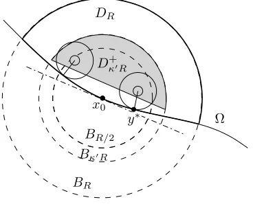
Definition 1.6. We say that Γ is C1,1 surface with radius ρ0 > 0 splitting B1 into Ω+ _{and Ω}− _{if the following happens.}

• The two disjoint domains Ω+ _{and Ω}− _partition _B

1, i.e., B1 = Ω+∪Ω−. • The boundary Γ :=∂Ω+_\_∂B

1 =∂Ω−\∂B1 is C1,1 surface with 0∈Γ. • All points on Γ∩B3/4 can be touched by two balls of radiiρ0, one contained

in Ω+ _{and the other contained in Ω}−_.

Theorem 1.7 ([E]). Let Γ be a C1,1 surface with radius ρ0 splitting B1 into Ω+

and Ω−; see Definition 1.6. Let d(x) = dist (x,Γ).

Let s0 ∈(0,1)and s∈[s0,1). Assume that I is a fully nonlinear and translation

invariant operator, elliptic with respect to L∗(s), with I0 = 0. Let f ∈C Ω+

, and

u∈L∞(_Rn₎_∩_C _Ω+

be a viscosity solution of

Iu = f in Ω+ u = 0 in Ω−.

Then, u/ds belongs to Cs− Ω+_∩_B 1/2

for all >0 with the estimate

u/ds

Cs−_(Ω+_∩B

1/2) ≤C kukL

∞_(Rn₎+kfk_L∞_(Ω+₎

,

(32)

30 INTRODUCTION

Theorem 1.7 is, to our knowledge, the first boundary regularity result for fully nonlinear integro-differential equations. For solutions u to elliptic equations with respect to L∗, our result gives a quite accurate description of the boundary behavior. Namely, u/ds isCs− for all >0, where d is the distance to the boundary.

We believe the H¨older exponents−in (1.23) to be optimal (or almost optimal) for merely bounded right hand sides f. Moreover, we expect the class L∗ to be the largest scale invariant subclass of L0 for which this result is true.

For general elliptic equations with respect to L0, no fine boundary regularity results like (1.23) hold. In fact, the class L0 is too large for all solutions to be comparable to ds _{near the boundary. Indeed, in [E] we show that there are powers} 0< β1 < s < β2 for which the functions (xn)+β1 and (xn)β+2 satisfy

M_L+

0(xn)

β1

+ = 0 and M − L0(xn)

β2

+ = 0 in {xn>0}, where M_L+

0 and M

−

L0 are the extremal operators for the class L0, Hence, since

(−∆)s_(x

n)s+ = 0 in {xn > 0}, we have at least three functions that solve fully nonlinear elliptic equations with respect to L0, but which are not even comparable near the boundary {xn = 0}. As we show in Section 2, the same happens for the subclasses L1 and L2 of L0 which have more regular kernels and were considered in [34, 35, 36].

It is important to notice that our result is not only an a priori estimate for classical solutions but also applies to viscosity solutions. For local equations of second order F(D2_{u) = 0, the boundary regularity for viscosity solutions to fully} nonlinear equations has been recently obtained by Silvestre-Sirakov [112].

Besides its own interest, the boundary regularity of solutions to integro-differential equations plays an important role in different contexts. For example, it is needed in overdetermined problems arising in shape optimization [52, 64] and also in Pohozaev-type or integration by parts identities [A]. Moreover, boundary regularity issues appear naturally in free boundary problems [32, 111].

Theorem 1.7 follows by combining an estimate on the boundary, (1.24) below, with the known interior regularity estimates in [34, 83]. The estimate on the bound-ary reads as follows. If u satisfies the hypotheses of Theorem 1.7, then for all z ∈Γ∩B1/2 there exists Q(z)∈R for which

u(x)−Q(z) (x−z)·ν(z) s

+

≤C|x−z| 2s−

for all x∈B1. (1.24) Here, ν(z) is the unit normal vector to Γ at z pointing towards Ω+.

From this point on, our proof differs substantially from that in second order equations. A main reason for this is not only the nonlocal character of the estimates, but also that tangential and normal derivatives of the solution behave differently on the boundary; recall that the solution is Cs _{but cannot be Lipschitz up to the} boundary.

(33)

The first ingredient is the following Liouville-type theorem for solutions in a half space.

Theorem 1.8 ([E]). Let u∈C(Rn) be a viscosity solution of

Iu = 0 in {xn >0} u = 0 in {xn <0},

where I is a fully nonlinear and translation invariant operator, elliptic with respect to L∗ and withI0 = 0. Assume that for some positive β <2s, u satisfies the growth control at infinity

kukL∞_(BR₎≤CRβ for all R ≥1. (1.25)

Then,

u(x) = K(xn)s+

for some constant K ∈_R.

The second ingredient towards (1.24) is a compactness argument, a boundary version of our interior regularity method for parabolic equations with rough kernels (see Section 1.7). With u as in Theorem 1.7, we suppose by contradiction that (1.24) does not hold, and we blow up the fully nonlinear equation at a boundary point (after subtracting appropriate terms to the solution). We then show that the solution converges to an entire solution in {x·ν >0}for some unit vectorν. Finally, the contradiction is reached by applying the Liouville-type theorem stated above to the entire solution in {x·ν >0}.

These are the main ideas used to prove (1.24). A byproduct of using this blow-up method is that the same proof yields results for non translation invariant equations. Finally, Theorem 1.7 follows by combining (1.24) with the interior regularity esti-mates in [34, 83].

1.9. Results: regularity of the fractional extremal solution. In the paper [F] of this thesis we study the extremal solution problem for the fractional Laplacian

(−∆)s_u ₌ _λf_{(u) in Ω}

u = 0 in _Rn_\Ω, (1.26)

where λ is a positive parameter and f : [0,∞)−→_R satisfies f isC1 and nondecreasing, f(0)>0, and lim

t→+∞ f(t)

t = +∞. (1.27)

It is well known —see [11] or the excellent monograph [60] and references therein— that in the classical case s = 1 there exists a finite extremal parame-ter λ∗ such that if 0 < λ < λ∗ then problem (1.26) admits a minimal classical solution uλ, while for λ > λ∗ it has no solution, even in the weak sense. Moreover, the family of functions {uλ : 0 < λ < λ∗} is increasing in λ, and its pointwise limit u∗ = limλ↑λ∗u_λ is a weak solution of problem (1.26) with λ = λ∗. It is called the

(34)

32 INTRODUCTION

When f(u) = eu_{, we have that} _u∗ _∈ _L∞_{(Ω) if} _n _≤ _{9 [50], while} _u∗_{(x) = log} 1 |x|2

if n ≥ 10 and Ω = B1 [80]. An analogous result holds for other nonlinearities such as powers f(u) = (1 +u)p _{and also for functions} _f _{satisfying a limit condition} at infinity; see [105]. In the nineties H. Brezis and J.L. Vázquez [11] raised the question of determining the regularity of u∗, depending on the dimension n, for general nonlinearitiesf satisfying (1.27). The first result in this direction was proved by G. Nedev [95], who obtained that the extremal solution is bounded in dimensions n ≤3 wheneverf is convex. Some years later, X. Cabré and A. Capella [19] studied the radial case. They showed that when Ω = B1 the extremal solution is bounded for all nonlinearities f whenever n ≤ 9. For general nonlinearities, the best known result at the moment is due to X. Cabré [18], and states that in dimensions n ≤ 4 then the extremal solution is bounded for any convex domain Ω —later, S. Villegas removed the convexity assumption on Ω.

In [F] we define an appropriate notion of weak solution for problem (1.26) and we prove the existence of a minimal branch of solutions, {uλ, 0 < λ < λ∗}, with the same properties as in the case s= 1. These solutions are proved to be positive, bounded, increasing in λ, and semistable. Recall that a weak solution uof (1.26) is said to be semistable if

Z Ω

λf0(u)η2dx≤ kηk2 ˚

Hs (1.28)

for all η ∈ Hs₍

Rn) with η ≡ 0 in Rn \Ω. When u is an energy solution this is equivalent to saying that the second variation of energy E atu is nonnegative.

The weak solution u∗ for λ = λ∗ is called the extremal solution of problem (1.26). As explained above, the main question about the extremal solution u∗ is to decide whether it is bounded or not. Once the extremal solution is bounded then it is a classical solution, in the sense that it satisfies equation (1.26) pointwise. For example, if f ∈C∞ then u∗ bounded yields u∗ ∈C∞(Ω)∩Cs(Ω).

Our main result, stated next, concerns the regularity of the extremal solution for problem (1.26). To our knowledge this is the first result concerning extremal solutions for (1.26). In particular, the following are new results even for the unit ball Ω = B1 and for the exponential nonlinearity f(u) =eu.

Theorem 1.9 ([F]). Let Ω be a bounded smooth domain in Rn, s∈(0,1), f be

a function satisfying (1.27), and u∗ be the extremal solution of (1.26).

(i) Assume that f is convex. Then, u∗ is bounded whenever n <4s.

(ii) Assume that f is C2 _{and that the following limit exists:} τ := lim

t→+∞

f(t)f00(t)

f0_(t)2 . (1.29)

Then, u∗ is bounded whenever n <10s.

(iii) Assume that Ωis convex. Then, u∗ belongs to Hs(_Rn) for all n≥1 and all

Elliptic and parabolic PDEs : regularity for nonlocal diffusion equations and two isoperimetric problems

Universitat Polit`

ecnica de Catalunya

Programa de Doctorat de Matem`

atica Aplicada

Departament de Matem`

atica Aplicada I

Elliptic and parabolic PDEs:

regularity for nonlocal diffusion equations

and two isoperimetric problems

by

Joaquim Serra

PhD dissertation

Acknowledgments

Summary

Contents

Introduction